CMB ANISOTROPIES: TOTAL ANGULAR MOMENTUM METHOD

Abstract

A total angular momentum representation simplifies the radiation transport problem for temperature and polarization anisotropy in the CMB. Scattering terms couple only the quadrupole moments of the distributions and each moment corresponds directly to the observable angular pattern on the sky. We develop and employ these techniques to study the general properties of anisotropy generation from scalar, vector and tensor perturbations to the metric and the matter, both in the cosmological fluids and from any seed perturbations (e.g. defects) that may be present. The simpler, more transparent form and derivation of the Boltzmann equations brings out the geometric and model-independent aspects of temperature and polarization anisotropy formation. Large angle scalar polarization provides a robust means to distinguish between isocurvature and adiabatic models for structure formation in principle. Vector modes have the unique property that the CMB polarization is dominated by magnetic type parity at small angles (a factor of $6$ in power compared with $0$ for the scalars and $8/13$ for the tensors) and hence potentially distinguishable independent of the model for the seed. The tensor modes produce a different sign from the scalars and vectors for the temperature-polarization correlations at large angles. We explore conditions under which one perturbation type may dominate over the others including a detailed treatment of the photon-baryon fluid before recombination.

Contents

toc

I Introduction

The cosmic microwave background (CMB) is fast becoming the premier laboratory for early universe and classical cosmology. With the flood of high quality data expected in the coming years, most notably from the new MAP [1] and Planck Surveyor [2] satellite missions, it is imperative that theoretical tools for their interpretation be developed. The corresponding techniques involved should be as physically transparent as possible so that the implications for cosmology will be readily apparent from the data.

Toward this end, we reconsider the general problem of temperature and polarization anisotropy formation in the CMB. These anisotropies arise from gravitational perturbations which separate into scalar (compressional), vector (vortical), and tensor (gravity wave) modes. In previous treatments, the simple underlying geometrical distinctions and physical processes involved in their appearance as CMB anisotropies has been obscured by the choice of representation for the angular distribution of the CMB. In this paper, we systematically develop a new representation, the total angular momentum representation, which puts vector and tensor modes for the temperature and all polarization modes on an equal footing with the familiar scalar temperature modes. For polarization, this completes and substantially simplifies the ground-breaking work of [3, 4]. Although we consider only flat geometries here for simplicity, the framework we establish allows for straightforward generalization to open geometries [5, 6, 7, 8] unlike previous treatments.

The central idea of this method is to employ only observable quantities, i.e. those which involve the total angular dependence of the temperature and polarization distributions. By applying this principle from beginning to end, we obtain a substantial simplification of the radiation transport problem underlying anisotropy formation. Scattering terms couple only the quadrupole moments of the temperature and polarization distributions. Each moment of the distribution corresponds to angular moments on the sky which allows a direct relation between the fundamental scattering and gravitational sources and the observable anisotropy through their integral solutions.

We study the means by which gravitational perturbations of the scalar, vector, or tensor type, originating in either the cosmological fluids or seed sources such as defects, form temperature and polarization anisotropies in the CMB. As is well established [3, 4], scalar perturbations generate only the so-called electric parity mode of the polarization. Here we show that conversely the ratio of magnetic to electric parity power is a factor of $6$ for vectors, compared with $8/13$ for tensors, independent of their source. Furthermore, the large angle limits of polarization must obey simple geometrical constraints for its amplitude that differ between scalars, vectors and tensors. The sense of the temperature-polarization cross correlation at large angle is also determined by geometric considerations which separate the scalars and vectors from the tensors [9]. These constraints are important since large-angle polarization unlike large-angle temperature anisotropies allow one to see directly scales above the horizon at last scattering. Combined with causal constraints, they provide robust signatures of causal isocurvature models for structure formation such as cosmological defects.

In §II we develop the formalism of the total angular momentum representation and lay the groundwork for the geometric interpretation of the radiation transport problem and its integral solutions. We further establish the relationship between scalars, vectors, and tensors and the orthogonal angular modes on the sphere. In §III, we treat the radiation transport problem from first principles. The total angular momentum representation simplifies both the derivation and the form of the evolution equations for the radiation. We present the differential form of these equations, their integral solutions, and their geometric interpretation. In §IV we specialize the treatment to the tight-coupling limit for the photon-baryon fluid before recombination and show how acoustic waves and vorticity are generated from metric perturbations and dissipated through the action of viscosity, polarization and heat conduction. In §V, we provide specific examples inspired by seeded models such as cosmological defects. We trace the full process that transfers seed fluctuations in the matter through metric perturbations to observable anisotropies in the temperature and polarization distributions.

II Normal Modes

In this section, we introduce the total angular momentum representation for the normal modes of fluctuations in a flat universe that are used to describe the CMB temperature and polarization as well as the metric and matter fluctuations. This representation greatly simplifies the derivation and form of the evolution equations for fluctuations in §III. In particular, the angular structure of modes corresponds directly to the angular distribution of the temperature and polarization, whereas the radial structure determines how distant sources contribute to this angular distribution.

The new aspect of this approach is the isolation of the total angular dependence of the modes by combining the intrinsic angular structure with that of the plane-wave spatial dependence. This property implies that the normal modes correspond directly to angular structures on the sky as opposed to the commonly employed technique that isolates portions of the intrinsic angular dependence and hence a linear combination of observable modes [10]. Elements of this approach can be found in earlier works (e.g. [6, 7, 11] for the temperature and [3] for the scalar and tensor polarization). We provide here a systematic study of this technique which also provides for a substantial simplification of the evolution equations and their integral solution in §III C, including the terms involving the radiation transport of the CMB. We discuss in detail how the monopole, dipole and quadrupole sources that enter into the radiation transport problem project as anisotropies on the sky today.

Readers not interested in the formal details may skip this section on first reading and simply note that the temperature and polarization distribution is decomposed into the modes $Y_{\ell}^{m}\exp(i\vec{k}\cdot\vec{x})$ and $\,{}_{\pm 2}^{\vphantom{m}}Y_{\ell}^{m}\exp(i\vec{k}\cdot\vec{x})$ with $m=0,\pm 1,\pm 2$ for scalar, vector and tensor metric perturbations respectively. In this representation, the geometric distinction between scalar, vector and tensor contributions to the anisotropies is clear as is the reason why they do not mix. Here the $\,{}_{\pm 2}^{\vphantom{m}}Y_{\ell}^{m}$ are the spin-2 spherical harmonics [12] and were introduced to the study of CMB polarization by [3]. The radial decompositions of the modes $Y_{\ell^{\prime}}^{m}j_{\ell^{\prime}}^{(\ell m)}(kr)$ and $\,{}_{\pm 2}^{\vphantom{m}}Y_{\ell^{\prime}}^{m}[\epsilon_{\ell^{\prime}}^{(m)}(kr)\pm i\beta_{\ell^{\prime}}^{(m)}(kr)]$ (for $\ell=2$) isolate the total angular dependence by combining the intrinsic and plane wave angular momenta.

A Angular Modes

In this section, we derive the basic properties of the angular modes of the temperature and polarization distributions that will be useful in §III to describe their evolution. In particular, the Clebsch-Gordan relation for the addition of angular momentum plays a central role in exposing the simplicity of the total angular momentum representation.

A scalar, or spin-$0$ field on the sky such as the temperature can be decomposed into spherical harmonics $Y_{\ell}^{m}$. Likewise a spin-$s$ field on the sky can be decomposed into the spin-weighted spherical harmonics $\,{}_{s}^{\vphantom{m}}Y_{\ell}^{m}$ and a tensor constructed out of the basis vectors $\hat{e}_{\theta}\pm i\hat{e}_{\phi}$, $\hat{e}_{r}$ [12]. The basis for a spin-2 field such as the polarization is $\,{}_{\pm 2}^{\vphantom{m}}Y_{\ell}^{m}{\bf M}_{\pm}$ [3, 4] where

$${\bf M}_{\pm}\equiv{1\over 2}(\hat{e}_{\theta}\mp i\hat{e}_{\phi})\otimes(\hat{e}_{\theta}\mp i\hat{e}_{\phi})\,,$$ (1)

since it transforms under rotations as a $2\times 2$ symmetric traceless tensor. This property is more easily seen through the relation to the Pauli matrices, ${\bf M}_{\pm}=\sigma_{3}\mp i\sigma_{1}$, in spherical coordinates $(\theta,\phi)$. The spin-$s$ harmonics are expressed in terms of rotation matrices as [12]

$$\,{}_{s}^{\vphantom{m}}Y_{\ell}^{m}(\theta,\phi) = \left({2\ell+1\over 4\pi}\right)^{1/2}{\cal D}_{-s,m}^{\ell}(\phi,\theta,0)\,$$ (2)

$$= \left[{2\ell+1\over 4\pi}{(\ell+m)!(\ell-m)!\over(\ell+s)!(\ell-s)!}\right]^{1/2}(\sin\theta/2)^{2\ell}\sum_{r}\left(\begin{array}[]{c}\ell-s\\ r\end{array}\right)\left(\begin{array}[]{c}\ell+s\\ r+s-m\end{array}\right)$$ (8)

$$\qquad\times(-1)^{\ell-r-s}e^{im\phi}(\cot\theta/2)^{2r+s-m}.$$

The rotation matrix ${\cal D}_{-s,m}^{\ell}(\phi,\theta,\psi)=\sqrt{4\pi/(2\ell+1)}\,{}_{s}^{\vphantom{m}}Y_{\ell}^{m}(\theta,\phi)e^{-is\psi}$ represents rotations by the Euler angles $(\phi,\theta,\psi)$. Since the spin-2 harmonics will be useful in the following sections, we give their explicit form in Table 1 for $\ell=2$; the higher $\ell$ harmonics are related to the ordinary spherical harmonics as

$$\,{}_{\pm 2}^{\vphantom{m}}Y_{\ell}^{m}=\left[{(\ell-2)!\over(\ell+2)!}\right]^{1/2}\left[\partial_{\theta}^{2}-{\rm cot}\theta\,\partial_{\theta}\pm{2i\over\sin\theta}(\partial_{\theta}-{\rm cot}\theta)\partial_{\phi}-{1\over\sin^{2}\theta}\partial^{2}_{\phi}\right]Y_{\ell}^{m}.$$ (9)

$m$	$Y_{2}^{m}$	$\,{}_{2}^{\vphantom{m}}Y_{2}^{m}$
2	${1\over 4}\sqrt{15\over 2\pi}\,\sin^{2}\theta\,e^{2i\phi}$	${1\over 8}\sqrt{5\over\pi}\,(1-\cos\theta)^{2}\,e^{2i\phi}$
1	$\sqrt{15\over 8\pi}\sin\theta\,\cos\theta\,e^{i\phi}$	${1\over 4}\sqrt{5\over\pi}\sin\theta\,(1-\cos\theta)\,e^{i\phi}$
0	${1\over 2}\sqrt{5\over 4\pi}\,(3\cos^{2}\theta-1)$	${3\over 4}\sqrt{5\over 6\pi}\,\sin^{2}\theta$
-1	$-\sqrt{15\over 8\pi}\sin\theta\,\cos\theta\,e^{-i\phi}$	${1\over 4}\sqrt{5\over\pi}\,\sin\theta\,(1+\cos\theta)\,e^{-i\phi}$
-2	${1\over 4}\sqrt{15\over 2\pi}\,\sin^{2}\theta\,e^{-2i\phi}$	${1\over 8}\sqrt{5\over\pi}\,(1+\cos\theta)^{2}\,e^{-2i\phi}$

TAB. 1: Quadrupole ($\ell=2$) harmonics for spin-$0$ and $2$.

By virtue of their relation to the rotation matrices, the spin harmonics satisfy: the compatibility relation with spherical harmonics, $\,{}_{0}^{\vphantom{m}}Y_{\ell}^{m}=Y_{\ell}^{m}$; the conjugation relation $\,{}_{s}^{\vphantom{m*}}Y_{\ell}^{m*}=(-1)^{m+s}\,{}_{-s}^{\vphantom{-m}}Y_{\ell}^{-m}$; the orthonormality relation,

$$\int d\Omega\,\left(\,{}_{s}^{\vphantom{m*}}Y_{\ell}^{m*}\right)\,\left(\,{}_{s}^{\vphantom{m}}Y_{\ell}^{m}\right)=\delta_{\ell,\ell^{\prime}}\delta_{m,m^{\prime}};$$ (10)

the completeness relation,

$$\sum_{\ell,m}\left[\,{}_{s}^{\vphantom{m*}}Y_{\ell}^{m*}(\theta,\phi)\right]\left[\,{}_{s}^{\vphantom{m}}Y_{\ell}^{m}(\theta^{\prime},\phi^{\prime})\right]=\delta(\phi-\phi^{\prime})\delta(\cos\theta-\cos\theta^{\prime})\,;$$ (11)

the parity relation,

$$\,{}_{s}^{\vphantom{m}}Y_{\ell}^{m}\rightarrow(-1)^{\ell}\,{}_{-s}^{\vphantom{m}}Y_{\ell}^{m};$$ (12)

the generalized addition relation,

$$\sum_{m}\left[\,{}_{s_{1}}^{\vphantom{m*}}Y_{\ell}^{m*}(\theta^{\prime},\phi^{\prime})\right]\left[\,{}_{s_{2}}^{\vphantom{m}}Y_{\ell}^{m}(\theta,\phi)\right]=\sqrt{2\ell+1\over 4\pi}\left[\,{}_{s_{2}}^{\vphantom{-s_{1}}}Y_{\ell}^{-s_{1}}(\beta,\alpha)\right]e^{-is_{2}\gamma}\,,$$ (13)

which follows from the group multiplication property of rotation matrices which relates a rotation from $(\theta^{\prime},\phi^{\prime})$ through the origin to $(\theta,\phi)$ with a direct rotation in terms of the Euler angles $(\alpha,\beta,\gamma)$ defined in Fig. 1; and the Clebsch-Gordan relation,

$$\left(\,{}_{s_{1}}^{\vphantom{m_{1}}}Y_{\ell_{1}}^{m_{1}}\right)\left(\,{}_{s_{2}}^{\vphantom{m_{2}}}Y_{\ell_{2}}^{m_{2}}\right) = {\sqrt{(2\ell_{1}+1)(2\ell_{2}+1)}\over 4\pi}\sum_{\ell,m,s}\left<\ell_{1},\ell_{2};m_{1},m_{2}|\ell_{1},\ell_{2};\ell,m\right>$$ (15)

$$\times\left<\ell_{1},\ell_{2};-s_{1},-s_{2}|\ell_{1},\ell_{2};\ell,-s\right>\sqrt{4\pi\over 2\ell+1}\,\left(\,{}_{s}^{\vphantom{m}}Y_{\ell}^{m}\right)\,.$$

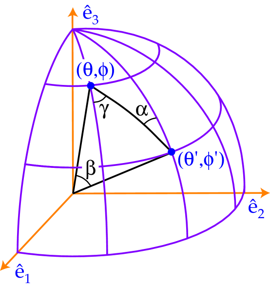
FIG. 1.: Addition theorem and scattering geometry. The addition theorem for spin-$s$ harmonics Eqn. (13) is established by their relation to rotations Eqn. (8) and by noting that a rotation from $(\theta^{\prime},\phi^{\prime})$ through the origin (pole) to $(\theta,\phi)$ is equivalent to a direct rotation by the Euler angles $(\alpha,\beta,\gamma)$. For the scattering problem of Eqn. (63), these angles represent the rotation by $\alpha$ from the $\hat{k}=\hat{e}_{3}$ frame to the scattering frame, by the scattering angle $\beta$, and by $\gamma$ back into the $\hat{k}$ frame.

It is worthwhile to examine the implications of these properties. Note that the orthogonality and completeness relations Eqns. (10) and (11) do not extend to different spin states. Orthogonality between $s=\pm 2$ states is established by the Pauli basis of Eqn. (1) ${\bf M}_{\pm}^{*}{\bf M}_{\pm}^{\vphantom{*}}={\bf 1}$ and ${\bf M}_{\pm}^{*}{\bf M}_{\mp}^{\vphantom{*}}={\bf 0}$. The parity equation (12) tells us that the spin flips under a parity transformation so that unlike the $s=0$ spherical harmonics, the higher spin harmonics are not parity eigenstates. Orthonormal parity states can be constructed as [3, 4]

$${1\over 2}[\,{}_{2}^{\vphantom{m}}Y_{\ell}^{m}{\bf M}_{+}\pm\,{}_{-2}^{\vphantom{m}}Y_{\ell}^{m}{\bf M}_{-}]\,,$$ (16)

which have “electric” $(-1)^{\ell}$ and “magnetic” $(-1)^{\ell+1}$ type parity for the $(\pm)$ states respectively. We shall see in §III C that the polarization evolution naturally separates into parity eigenstates. The addition property will be useful in relating the scattering angle to coordinates on the sphere in §III B. Finally the Clebsch-Gordan relation Eqn. (15) is central to the following discussion and will be used to derive the total angular momentum representation in §II B and evolution equations for angular moments of the radiation §III C.

B Radial Modes

We now complete the formalism needed to describe the temperature and polarization fields by adding a spatial dependence to the modes. By further separating the radial dependence of the modes, we gain insight on their full angular structure. This decomposition will be useful in constructing the formal integral solutions of the perturbation equations in §III C. We begin with its derivation and then proceed to its geometric interpretation.

1 Derivation

The temperature and polarization distribution of the radiation is in general a function of both spatial position $\vec{x}$ and angle $\vec{n}$ defining the propagation direction. In flat space, we know that plane waves form a complete basis for the spatial dependence. Thus a spin-$0$ field like the temperature may be expanded in

$$G_{\ell}^{m}=(-i)^{\ell}\sqrt{4\pi\over 2\ell+1}Y_{\ell}^{m}(\hat{n})\exp(i\vec{k}\cdot\vec{x})\,,$$ (17)

where the normalization is chosen to agree with the standard Legendre polynomial conventions for $m=0$. Likewise a spin-$2$ field like the polarization may be expanded in

$${}_{\pm 2}G_{\ell}^{m}=(-i)^{\ell}\sqrt{{4\pi\over 2\ell+1}}[\,{}_{\pm 2}^{\vphantom{m}}Y_{\ell}^{m}(\hat{n})]\exp(i\vec{k}\cdot\vec{x})\,.$$ (18)

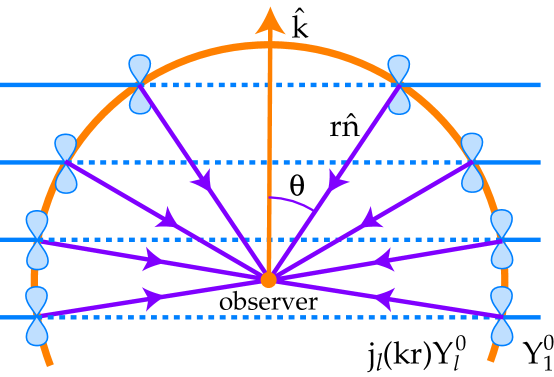
FIG. 2.: Projection effects. A plane wave $\exp(i\vec{k}\cdot\vec{x})$ can be decomposed into $j_{\ell}(kr)Y_{\ell}^{0}$ and hence carries an “orbital” angular dependence. A plane wave source at distance $r$ thus contributes angular power to $\ell\approx kr$ at $\theta=\pi/2$ but also to larger angles $\ell\ll kr$ at $\theta=0$ which is encapsulated into the structure of $j_{\ell}$ (see Fig. 3). If the source has an intrinsic angular dependence, the distribution of power is altered. For an aligned dipole $Y_{1}^{0}\propto\cos\theta$ (‘figure 8’s) power at $\theta=\pi/2$ or $\ell\approx kr$ is suppressed. These arguments are generalized for other intrinsic angular dependences in the text.

The plane wave itself also carries an angular dependence of course,

$$\exp(i\vec{k}\cdot\vec{x})=\sum_{\ell}(-i)^{\ell}\sqrt{4\pi(2\ell+1)}j_{\ell}(kr)Y_{\ell}^{0}(\hat{n})\,,$$ (19)

where $\hat{e}_{3}=\hat{k}$ and $\vec{x}=-r\hat{n}$ (see Fig. 2). The sign convention for the direction is opposite to direction on the sky to be in accord with the direction of propagation of the radiation to the observer. Thus the extra factor of $(-1)^{\ell}$ comes from the parity relation Eqn. (12).

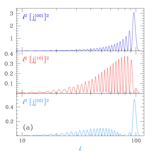
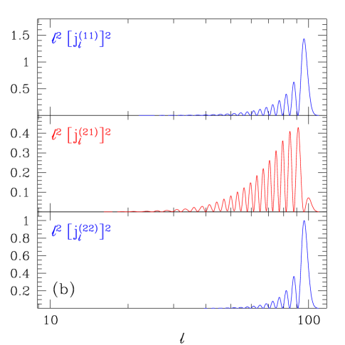
FIG. 3.: Radial spin-0 (temperature) modes. The angular power in a plane wave (left panel, top) is modified due to the intrinsic angular structure of the source as discussed in the text. The left panel corresponds to the power in scalar ($m=0$) monopole $G_{0}^{0}$, dipole $G_{1}^{0}$, and quadrupole $G_{2}^{0}$ sources (top to bottom); the right panel to that in vector ($m=1$) dipole $G_{1}^{\pm 1}$ and quadrupole $G_{2}^{\pm 1}$ sources and a tensor ($m=2$) quadrupole $G_{2}^{\pm 2}$ source (top to bottom). Note the differences in how sharply peaked the power is at $\ell\approx kr$ and how fast power falls as $\ell\ll kr$. The argument of the radial functions $kr=100$ here.

The separation of the mode functions into an intrinsic angular dependence and plane-wave spatial dependence is essentially a division into spin ($\,{}_{s}^{\vphantom{m}}Y_{\ell^{\prime}}^{m}$) and orbital ($Y_{\ell}^{0}$) angular momentum. Since only the total angular dependence is observable, it is instructive to employ the Clebsch-Gordan relation of Eqn. (15) to add the angular momenta. In general this couples the states between $|\ell-\ell^{\prime}|$ and $\ell+\ell^{\prime}$. Correspondingly a state of definite total $\ell$ will correspond to a weighted sum of $j_{|\ell-\ell^{\prime}|}$ to $j_{\ell+\ell^{\prime}}$ in its radial dependence. This can be reexpressed in terms of the $j_{\ell}$ using the recursion relations of spherical Bessel functions,

$${j_{\ell}(x)\over x} = {1\over 2\ell+1}[j_{\ell-1}(x)+j_{\ell+1}(x)]\,,$$ (20)

$$j_{\ell}^{\prime}(x) = {1\over 2\ell+1}[\ell j_{\ell-1}(x)-(\ell+1)j_{\ell+1}(x)]\,.$$ (21)

We can then rewrite

$$G_{\ell^{\prime}}^{m}=\sum_{\ell}(-i)^{\ell}\sqrt{4\pi(2\ell+1)}\,j_{\ell}^{(\ell^{\prime}m)}(kr)\,Y_{\ell}^{m}(\hat{n})\,,$$ (22)

where the lowest $(\ell^{\prime},m)$ radial functions are

$$\begin{array}[]{lll}j_{\ell}^{(00)}(x)=j_{\ell}(x)\,,&j_{\ell}^{(10)}(x)=j_{\ell}^{\prime}(x)\,,&j_{\ell}^{(20)}(x)={1\over 2}[3j_{\ell}^{\prime\prime}(x)+j_{\ell}(x)]\,,\vphantom{\Bigg{[}}\\ &j_{\ell}^{(11)}(x)=\displaystyle{\sqrt{\ell(\ell+1)\over 2}\,{j_{\ell}(x)\over x}}\,,&j_{\ell}^{(21)}(x)=\displaystyle{\sqrt{3\ell(\ell+1)\over 2}\,\left({j_{\ell}(x)\over x}\right)^{\prime}}\,,\vphantom{\Bigg{[}}\\ &&j_{\ell}^{(22)}(x)=\displaystyle{\sqrt{{3\over 8}{(\ell+2)!\over(\ell-2)!}}\,{j_{\ell}(x)\over x^{2}}}\vphantom{\Bigg{[}},\end{array}$$ (23)

with primes representing derivatives with respect to the argument of the radial function $x=kr$. These modes are shown in Fig. 3.

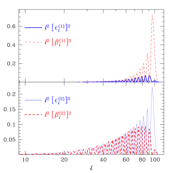
FIG. 4.: Radial spin-2 (polarization) modes. Displayed is the angular power in a plane-wave spin-2 source. The top panel shows that vector ($m=1$, upper panel) sources are dominated by $B$-parity contributions, whereas tensor ($m=2$, lower panel) sources have comparable but less power in the $B$-parity. Note that the power is strongly peaked at $\ell=kr$ for the $B$-parity vectors and $E$-parity tensors. The argument of the radial functions $kr=100$ here.

Similarly for the spin $\pm 2$ functions with $m>0$ (see Fig. 4),

$${}_{\pm 2}G_{2}^{m}=\sum_{\ell}(-i)^{\ell}\sqrt{4\pi(2\ell+1)}[\epsilon_{\ell}^{(m)}(kr)\pm i\beta_{\ell}^{(m)}(kr)]\,\,{}_{\pm 2}^{\vphantom{m}}Y_{\ell}^{m}(\hat{n})\,,$$ (24)

where

$$\epsilon^{(0)}_{\ell}(x) = \sqrt{{3\over 8}{(\ell+2)!\over(\ell-2)!}}{j_{\ell}(x)\over x^{2}}\,,\vphantom{\displaystyle{\dot{a}\over a}}$$ (25)

$$\epsilon^{(1)}_{\ell}(x) = {1\over 2}\sqrt{(\ell-1)(\ell+2)}\left[{j_{\ell}(x)\over x^{2}}+{j_{\ell}^{\prime}(x)\over x}\right]\,,$$ (26)

$$\epsilon^{(2)}_{\ell}(x) = {1\over 4}\left[-j_{\ell}(x)+j_{\ell}^{\prime\prime}(x)+2{j_{\ell}(x)\over x^{2}}+4{j_{\ell}^{\prime}(x)\over x}\right]\,,$$ (27)

which corresponds to the $\ell^{\prime}=\ell,\ell\pm 2$ coupling and

$$\beta^{(0)}_{\ell}(x) = 0\,,$$ (28)

$$\beta^{(1)}_{\ell}(x) = {1\over 2}\sqrt{(\ell-1)(\ell+2)}{j_{\ell}(x)\over x}\,,$$ (29)

$$\beta^{(2)}_{\ell}(x) = {1\over 2}\left[j_{\ell}^{\prime}(x)+2{j_{\ell}(x)\over x}\right]\,,$$ (30)

which corresponds to the $\ell^{\prime}=\ell\pm 1$ coupling. The corresponding relation for negative $m$ involves a reversal in sign of the $\beta$-functions

$$\epsilon_{\ell}^{(-m)} = \epsilon_{\ell}^{(m)},$$ (31)

$$\beta_{\ell}^{(-m)} = -\beta_{\ell}^{(m)}.$$ (32)

These functions are plotted in Fig. 4. Note that $\epsilon^{(0)}_{\ell}=j^{(2)}_{\ell}$ is displayed in Fig. 3.

2 Interpretation

The structure of these functions is readily apparent from geometrical considerations. A single plane wave contributes to a range of angular scales from $\ell\approx kr$ at $\theta=\pi/2$ to larger angles $\ell\ll kr$ as $\theta\rightarrow(0,\pi)$, where $\hat{k}\cdot\hat{n}=\cos\theta$ (see Fig. 1). The power in $\ell$ of a single plane wave shown in Fig. 3(a) (top panel) drops to zero $\ell\gtrsim kr$, has a concentration of power around $\ell=kr$ and an extended low amplitude tail to $\ell\lesssim kr$.

Now if the plane wave is multiplied by an intrinsic angular dependence, the projected power changes. The key to understanding this effect is to note that the intrinsic angular behavior is related to power in $\ell$ as

$$\theta\rightarrow(0,\pi)\qquad \Longleftrightarrow \qquad\ell\ll kr\,,$$ (33)

$$\theta\rightarrow\pi/2\qquad \Longleftrightarrow \qquad\ell\approx kr\,.$$ (34)

Thus factors of $\sin\theta$ in the intrinsic angular dependence suppress power at $\ell\ll kr$ (“aliasing suppression”), whereas factors of $\cos\theta$ suppress power at $\ell\approx kr$ (“projection suppression”). Let us consider first a $m=0$ dipole contribution $Y_{1}^{0}\propto\cos\theta$ (see Fig. 2). The $\cos\theta$ dependence suppresses power in $j_{\ell}^{(10)}$ at the peak in the plane-wave spectrum $\ell\approx kr$ (compare Fig. 3(a) top and middle panels). The remaining power is broadly distributed for $\ell\lesssim kr$. The same reasoning applies for $Y_{2}^{0}$ quadrupole sources which have an intrinsic angular dependence of $3\cos^{2}\theta-1$. Now the minimum falls at $\theta=\cos^{-1}(1/\sqrt{3})$ causing the double peaked form of the power in $j_{\ell}^{(20)}$ shown in Fig. 3(a) (bottom panel). This series can be continued to higher $G_{\ell}^{0}$ and such techniques have been used in the free streaming limit for temperature anisotropies [11].

Similarly, the structures of $j_{\ell}^{(11)}$, $j_{\ell}^{(21)}$ and $j_{\ell}^{(22)}$ are apparent from the intrinsic angular dependences of the $G_{1}^{1}$, $G_{2}^{1}$ and $G_{2}^{2}$ sources,

$$Y_{1}^{1}\propto\sin\theta e^{i\phi}\,,\qquad Y_{2}^{1}\propto\sin\theta\cos\theta e^{i\phi}\,,\qquad Y_{2}^{2}\propto\sin^{2}\theta e^{2i\phi}\,,$$ (35)

respectively. The $\sin\theta$ factors imply that as $m$ increases, low $\ell$ power in the source decreases (compare Fig. 3(a,b) top panels). $G_{2}^{1}$ suffers a further suppression at $\theta=\pi/2$ $(\ell\approx kr)$ from its $\cos\theta$ factor.

There are two interesting consequences of this behavior. The sharpness of the radial function around $\ell=kr$ quantifies how faithfully features in the $k$-space spectrum are preserved in $\ell$-space. If all else is equal, this faithfulness increases with $|m|$ for $G_{|m|}^{m}$ due to aliasing suppression from $\sin^{m}\theta.$ On the other hand, features in $G_{|m|+1}^{m}$ are washed out in comparison due projection suppression from the $\cos\theta$ factor.

Secondly, even if there are no contributions from long wavelength sources with $k\ll\ell/r$, there will still be large angle anisotropies at $\ell\ll kr$ which scale as

$$[\ell j_{\ell}^{(\ell^{\prime}m)}]^{2}\propto\ell^{2+2|m|}.$$ (36)

This scaling puts an upper bound on how steeply the power can rise with $\ell$ that increases with $|m|$ and hence a lower bound on the amount of large relative to small angle power that decreases with $|m|$.

The same arguments apply to the spin-$2$ functions with the added complication of the appearance of two radial functions $\epsilon_{\ell}$ and $\beta_{\ell}$. The addition of spin-2 angular momenta introduces a $\beta$-contribution from $e^{im\phi}$ except for $m=0$. For $m=\pm 1$, the $\beta$-contribution strongly dominates over the $\epsilon$-contributions; whereas for $m=\pm 2$, $\epsilon$-contributions are slightly larger than $\beta$-contributions (see Fig. 4). The ratios reach the asymptotic values of

$${\sum_{\ell}[\ell\beta_{\ell}^{(m)}]^{2}\over\sum_{\ell}[\ell\epsilon_{\ell}^{(m)}]^{2}}\approx\cases{6,&$m=\pm 1,$\cr 8/13,&$m=\pm 2,$\cr}$$ (37)

for fixed $kr\gg 1$. These considerations are closely related to the parity of the multipole expansion. Although the orbital angular momentum does not mix states of different spin, it does mix states of different parity since the plane wave itself does not have definite parity. A state with “electric” parity in the intrinsic angular dependence (see Eqn. 16) becomes

$${}_{2}^{\vphantom{2}}G_{2}^{m}{\bf M}_{+}+{}_{-2}^{\vphantom{2}}G_{2}^{m}{\bf M}_{-} = \sum_{\ell}(-i)^{\ell}\sqrt{4\pi(2\ell+1)}\Big{\{}\epsilon_{\ell}^{(m)}[\,{}_{2}^{\vphantom{m}}Y_{\ell}^{m}{\bf M}_{+}+\,{}_{-2}^{\vphantom{m}}Y_{\ell}^{m}{\bf M}_{-}]$$ (39)

$$\qquad+i\beta_{\ell}^{(m)}[\,{}_{2}^{\vphantom{m}}Y_{\ell}^{m}{\bf M}_{+}-\,{}_{-2}^{\vphantom{m}}Y_{\ell}^{m}{\bf M}_{-}]\Big{\}}.$$

Thus the addition of angular momentum of the plane wave generates “magnetic” $B$-type parity of amplitude $\beta_{\ell}$ out of an intrinsically “electric” $E$-type source as well as $E$-type parity of amplitude $\epsilon_{\ell}$. Thus the behavior of the two radial functions has significant consequences for the polarization calculation in §III C and implies that B-parity polarization is absent for scalars, dominant for vectors, and comparable to but slightly smaller than the E-parity for tensors.

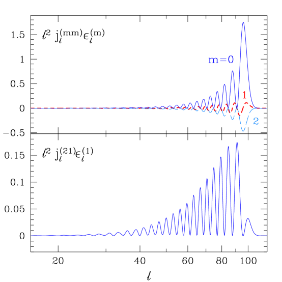
FIG. 5.: Spin-0 $\times$ Spin-2 (temperature $\times$ polarization) modes. Displayed is the cross angular power in plane wave spin-0 and spin-2 sources. The top panel shows that a scalar monopole ($m=0$) source correlates with a scalar spin-2 (polarization quadrupole) source whereas the tensor quadrupole ($m=2$) anticorrelates with a tensor spin-2 source. Vector dipole ($m=1$) sources oscillate in their correlation with vector spin-2 sources and contribute negligible once modes are superimposed. One must go to vector quadrupole sources (lower panel) for a strong correlation. The argument of the radial functions $kr=100$ here.

Now let us consider the low $\ell\ll kr$ tail of the spin-$2$ radial functions. Unlike the spin-0 projection, the spin-2 projection allows increasingly more power at $\theta\rightarrow 0$ and/or $\pi$, i.e. $\ell\ll kr$, as $|m|$ increases (see Table 1 and note the factors of $\sin\theta$). In this limit, the power in a plane wave fluctuation goes as

$$[\ell\epsilon_{\ell}^{(m)}]^{2}\propto\ell^{6-2|m|},\qquad[\ell\beta_{\ell}^{(m)}]^{2}\propto\ell^{6-2|m|}.$$ (40)

Comparing these expressions with Eqn. (36), we note that the spin-$0$ and spin-$2$ functions have an opposite dependence on $m$. The consequence is that the relative power in large vs. small angle polarization tends to decrease from the $m=2$ tensors to the $m=0$ scalars.

Finally it is interesting to consider the cross power between spin-$0$ and spin-$2$ sources because it will be used to represent the temperature-polarization cross correlation. Again interesting geometric effects can be identified (see Fig. 5). For $m=0$, the power in $j_{\ell}^{(00)}\epsilon_{\ell}^{(0)}$ correlates (Fig. 5, top panel solid line, positive definite); for $m=1$, $j_{\ell}^{(11)}\epsilon_{\ell}^{(1)}$ oscillates (short dashed line) and for $m=2$, $j_{\ell}^{(22)}\epsilon_{\ell}^{(2)}$ anticorrelates (long dashed line, negative definite). The cross power involves only $\epsilon_{\ell}^{(m)}j_{\ell}^{(\ell^{\prime}m)}$ due to the opposite parity of the $\beta_{\ell}^{(m)}$ modes.

These properties will become important in §III and IV B and translates into cross power contributions with opposite sign between the scalar monopole temperature cross polarization sources and tensor quadrupole temperature cross polarization sources [9]. Vector dipole temperature and polarization sources do not contribute strongly to the cross power since correlations and anticorrelations in $j_{\ell}^{(11)}\epsilon_{\ell}^{(1)}$ will cancel when modes are superimposed. The same is true of the scalar dipole temperature cross polarization $j_{\ell}^{(10)}\epsilon_{\ell}^{(0)}$ as is apparent from Figs. 3 and 4. The vector cross power is dominated by quadrupole temperature and polarization sources $j_{\ell}^{(21)}\epsilon_{\ell}^{(1)}$ (Fig. 5 lower panel).

C Perturbation Classification

As is well known (see e.g. [7, 15]), a general symmetric tensor such as the metric and stress-energy perturbations can be separated into scalar, vector and tensor pieces through their coordinate transformation properties. We now review the properties of their normal modes so that they may be related to those of the radiation. We find that the $m=0,\pm 1,\pm 2$ modes of the radiation couple to the scalar, vector and tensor modes of the metric. Although we consider flat geometries here, we preserve a covariant notation that ensures straightforward generalization to open geometries through the replacement of $\delta_{ij}$ with the curved three metric and ordinary derivatives with covariant derivatives [6, 7].

1 Scalar Perturbations

Scalar perturbations in a flat universe are represented by plane waves $Q^{(0)}=\exp(i\vec{k}\cdot\vec{x})$, which are the eigenfunctions of the Laplacian operator

$$\nabla^{2}Q^{(0)}=-k^{2}Q^{(0)},$$ (41)

and their spatial derivatives. For example, vector and symmetric tensor quantities such as velocities and stresses based on scalar perturbations can be constructed as

$$Q_{i}^{(0)}=-k^{-1}\nabla_{i}Q^{(0)},\qquad Q_{ij}^{(0)}=[k^{-2}\nabla_{i}\nabla_{j}+{1\over 3}\delta_{ij}]Q^{(0)}.$$ (42)

Since $\vec{\nabla}\times\vec{Q}^{(0)}=0$, velocity fields based on scalar perturbations are irrotational. Notice that $Q^{(0)}=G_{0}^{0}$, ${n}^{i}Q_{i}^{(0)}=G_{1}^{0}$ and ${n}^{i}{n}^{j}Q_{ij}^{(0)}\propto G_{2}^{0}$, where the coordinate system is defined by $\hat{e}_{3}=\hat{k}$. From the orthogonality of the spherical harmonics, it follows that scalars generate only $m=0$ fluctuations in the radiation.

2 Vector Perturbations

Vector perturbations can be decomposed into harmonic modes $Q^{(\pm 1)}_{i}$ of the Laplacian in the same manner as the scalars,

$$\nabla^{2}Q^{(\pm 1)}_{i}=-k^{2}Q^{(\pm 1)}_{i},$$ (43)

which satisfy a divergenceless condition

$${\nabla}^{i}{Q}_{i}^{(\pm 1)}=0\,.$$ (44)

A velocity field based on vector perturbations thus represents vorticity, whereas scalar objects such as density perturbations are entirely absent. The corresponding symmetric tensor is constructed out of derivatives as

$$Q_{ij}^{(\pm 1)}=-{1\over 2k}(\nabla_{i}Q_{j}^{(\pm 1)}+\nabla_{j}Q_{i}^{(\pm 1)})\,.$$ (45)

A convenient representation is

$${Q}_{i}^{(\pm 1)}=-{i\over\sqrt{2}}(\hat{e}_{1}\pm i\hat{e}_{2})_{i}\exp(i\vec{k}\cdot\vec{x})\,.$$ (46)

Notice that $n^{i}Q_{i}^{(\pm 1)}=G_{1}^{\pm 1}$ and $n^{i}n^{j}Q_{ij}^{(\pm 1)}\propto G_{2}^{\pm 1}$. Thus vector perturbations stimulate the $m=\pm 1$ modes in the radiation.

3 Tensor Perturbations

Tensor perturbations are represented by Laplacian eigenfunctions

$$\nabla^{2}Q_{ij}^{(\pm 2)}=-k^{2}Q_{ij}^{(\pm 2)},$$ (47)

which satisfy a transverse-traceless condition

$$\delta^{ij}Q^{(\pm 2)}_{ij}=\nabla^{i}Q^{(\pm 2)}_{ij}{}=0\,,$$ (48)

that forbids the construction of scalar and vector objects such as density and velocity fields. The modes take on an explicit representation of

$${Q}_{ij}^{(\pm 2)}=-\sqrt{3\over 8}(\hat{e}_{1}\pm i\hat{e}_{2})_{i}\otimes(\hat{e}_{1}\pm i\hat{e}_{2})_{j}\exp(i\vec{k}\cdot\vec{x})\,.$$ (49)

Notice that $n^{i}n^{j}Q_{ij}^{(\pm 2)}=G_{2}^{\pm 2}$ and thus tensors stimulate the $m=\pm 2$ modes in the radiation.

In the following sections, we often only explicitly show the positive $m$ value with the understanding that its opposite takes on the same form except where otherwise noted (i.e. in the $B$-type polarization where a sign reversal occurs).

III Perturbation Evolution

We discuss here the evolution of perturbations in the normal modes of §II. We first review the decomposition of perturbations in the metric and stress-energy tensor into scalar, vector and tensor types (§III A). We further divide the stress-energy tensor into fluid contributions, applicable to the usual particle species, and seed perturbations, applicable to cosmological defect models. We then employ the techniques developed in §II to obtain a new, simpler derivation and form of the radiation transport of the CMB under Thomson scattering, including polarization (§III B), than that obtained first by [16]. The complete evolution equations, given in §III C, are again substantially simpler in form than those of prior works where they overlap [3, 4, 10, 11] and treats the case of vector perturbations. Finally in §III D, we derive the formal integral solutions through the use of the radial functions of §II B and discuss their geometric interpretation. These solutions encapsulate many of the important results.

A Perturbations

1 Metric Tensor

The ultimate source of CMB anisotropies is the gravitational redshift induced by the metric fluctuation $h_{\mu\nu}$

$$g_{\mu\nu}=a^{2}(\eta_{\mu\nu}+h_{\mu\nu})\,,$$ (50)

where the zeroth component represents conformal time $d\eta=dt/a$ and, in the flat universe considered here, $\eta_{\mu\nu}$ is the Minkowski metric. The metric perturbation can be further broken up into the normal modes of scalar, vector and tensor types as in §II C. Scalar and vector modes exhibit gauge freedom which is fixed by an explicit choice of the coordinates that relate the perturbation to the background. For the scalars, we choose the Newtonian gauge (see e.g. [15, 17])

$$h_{00}=2\Psi Q^{(0)},\qquad h_{ij}=2\Phi Q^{(0)}\delta_{ij}\,,$$ (51)

where the metric is shear free. For the vectors, we choose

$$h_{0i}=-VQ_{i}^{(1)},$$ (52)

and the tensors

$$h_{ij}=2HQ_{ij}^{(2)}.$$ (53)

Note that tensor fluctuations do not exhibit gauge freedom of this type.

2 Stress Energy Tensor

The stress energy tensor can be broken up into fluid ($f$) contributions and seed ($s$) contributions (see e.g. [18]). The latter is distinguished by the fact that the net effect can be viewed as a perturbation to the background. Specifically $T_{\mu\nu}=\bar{T}_{\mu\nu}+\delta T_{\mu\nu}$ where $\bar{T}^{0}_{\hphantom{0}0}=-\rho_{f}$, $\bar{T}^{0}_{\hphantom{0}i}=\bar{T}_{0}^{\hphantom{i}i}=0$ and $\bar{T}^{i}_{\hphantom{i}j}=p_{f}\delta^{i}{}_{j}$ is given by the fluid alone. The fluctuations can be decomposed into the normal modes of §II C as

$$\begin{array}[]{lcl}\delta T^{0}_{\hphantom{0}0}&=&-[\rho_{f}\delta_{f}+\rho_{s}]\,Q^{(0)},\vphantom{\displaystyle{\dot{a}\over a}}\\ \delta T^{0}_{\hphantom{0}i}&=&[(\rho_{f}+p_{f})v_{f}^{(0)}+v_{s}^{(0)}]\,Q_{i}^{(0)},\vphantom{\displaystyle{\dot{a}\over a}}\\ \delta T_{0}^{\hphantom{i}i}&=&-[(\rho_{f}+p_{f})v_{f}^{(0)}+v_{s}^{(0)}]\,Q^{(0)}{}^{i},\vphantom{\displaystyle{\dot{a}\over a}}\\ \delta T^{i}_{\hphantom{i}j}&=&[\delta p_{f}+p_{s}\delta^{i}_{\hphantom{i}j}]Q^{(0)}+[p_{f}\pi_{f}+p_{s}]Q^{(0)}{}^{i}_{\hphantom{i}j}\vphantom{\displaystyle{\dot{a}\over a}}\,.\end{array}$$ (54)

for the scalar components,

$$\begin{array}[]{rcl}\delta T^{i}_{\hphantom{0}0}&=&-[(\rho_{f}+p_{f})v_{f}^{(1)}+\rho_{s}]\,Q^{{(1)}\,i},\vphantom{\displaystyle{\dot{a}\over a}}\\ \delta T^{0}_{\hphantom{0}i}&=&[(\rho_{f}+p_{f})(v_{f}^{(1)}-V)+v_{s}^{(1)}]\,Q^{(1)}_{i},\vphantom{\displaystyle{\dot{a}\over a}}\\ \delta T^{i}_{\hphantom{0}j}&=&[p_{f}\pi_{f}^{(1)}+\pi_{s}^{(1)}]\,Q^{(1)}{}^{i}_{\hphantom{i}j}\vphantom{\displaystyle{\dot{a}\over a}}\,,\end{array}$$ (55)

for the vector components, and

$$\delta T^{i}_{\hphantom{0}j}=[p_{f}\pi_{f}^{{(2)}}+\pi_{s}^{(2)}]\,Q^{(2)}{}^{i}_{\hphantom{i}j}\,,$$ (56)

for the tensor components.

B Radiation Transport

1 Stokes Parameters

The Boltzmann equation for the CMB describes the transport of the photons under Thomson scattering by the electrons. The radiation is described by the intensity matrix: the time average of the electric field tensor $E_{i}^{*}E_{j}$ over a time long compared to the frequency of the light or equivalently as the components of the photon density matrix (see [19] for reviews). For radiation propagating radially $\vec{E}\perp\hat{e}_{r}$, so that the intensity matrix exists on the $\hat{e}_{\theta}\otimes\hat{e}_{\phi}$ subspace. The matrix can further be decomposed in terms of the $2\times 2$ Pauli matrices $\sigma_{i}$ and the unit matrix ${\bf 1}$ on this subspace.

For our purposes, it is convenient to describe the polarization in temperature fluctuation units rather than intensity, where the analogous matrix becomes,

$${\bf T}=\Theta{\bf 1}+Q\sigma_{3}+U\sigma_{1}+V\sigma_{2}.$$ (57)

$\Theta={\rm Tr}({\bf T}{\bf 1})/2=\Delta T/T$ is the temperature perturbation summed over polarization states. Since $Q={\rm Tr}({\bf T}\sigma_{3})/2$, it is the difference in temperature fluctuations polarized in the $\hat{e}_{\theta}$ and $\hat{e}_{\phi}$ directions. Similarly $U={\rm Tr}({\bf T}\sigma_{1})/2$ is the difference along axes rotated by 45^∘, $(\hat{e}_{\theta}\pm\hat{e}_{\phi})/\sqrt{2}$, and $V={\rm Tr}({\bf T}\sigma_{2})/2$ that between $(\hat{e}_{\theta}\pm i\hat{e}_{\phi})/\sqrt{2}$. $Q$ and $U$ thus represent linearly polarized light in the north/south–east/west and northeast/southwest–northwest/southeast directions on the sphere respectively. $V$ represents circularly polarized light (in this section only, not to be confused with vector metric perturbations).

Under a counterclockwise rotation of the axes through an angle $\psi$ the intensity ${\bf T}$ transforms as ${\bf T}^{\prime}={\bf R}{\bf T}{\bf R}^{-1}$. $\Theta$ and $V$ remain distinct while $Q$ and $U$ transform into one another. Since the Pauli matrices transform as $\sigma_{3}^{\prime}\pm i\sigma_{1}^{\prime}=e^{\mp 2i\psi}(\sigma_{3}\pm i\sigma_{1})$ a more convenient description is

$${\bf T}=\Theta{\bf 1}+V\sigma_{2}+(Q+iU){\bf M}_{+}+(Q-iU){\bf M}_{-}\,,$$ (58)

where recall that ${\bf M}_{\pm}=(\sigma_{3}\mp i\sigma_{1})/2$ (see Eqn. 1), so that $Q\pm iU$ transforms into itself under rotation. Thus Eqn. (8) implies that $Q\pm iU$ should be decomposed into $s=\pm 2$ spin harmonics [3, 4].

Since circular polarization cannot be generated by Thomson scattering alone, we shall hereafter ignore $V$. It is then convenient to reexpress the matrix as a vector

$$\vec{T}=(\Theta,Q+iU,Q-iU)\,.$$ (59)

The Boltzmann equation describes the evolution of the vector $\vec{T}$ under the Thomson collisional term $C[\vec{T}]$ and gravitational redshifts in a perturbed metric $G[h_{\mu\nu}]$

$${d\over d\eta}\vec{T}(\eta,\vec{x},\hat{n})\equiv{\partial\over\partial\eta}\vec{T}+n^{i}\nabla_{i}\vec{T}=\vec{C}[{\vec{T}}]+\vec{G}[h_{\mu\nu}]\,,$$ (60)

where we have used the fact that $\dot{x}_{i}=n_{i}$ and that in a flat universe photons propagate in straight lines $\dot{n}=0$. We shall now evaluate the Thomson scattering and gravitational redshift terms.

2 Scattering Matrix

The calculation of Thomson scattering including polarization was first performed by Chandrasekhar [16]; here we show a much simpler derivation employing the spin harmonics. The Thomson differential scattering cross section depends on angle as $|\hat{\epsilon}^{\prime}\cdot\hat{\epsilon}|^{2}$ where $\hat{\epsilon}^{\prime}$ and $\hat{\epsilon}$ are the incoming and outgoing polarization vectors respectively in the electron rest frame. Radiation polarized perpendicular to the scattering plane scatters isotropically, while that in the scattering plane picks up a factor of $\cos^{2}\beta$ where $\beta$ is the scattering angle. If the radiation has different intensities or temperatures at right angles, the radiation scattered into a given angle will be linearly polarized.

Now let us evaluate the scattering term explicitly. The angular dependence of the scattering gives

$$\left(\begin{array}[]{c}\Theta_{\parallel}\\ \Theta_{\perp}\\ U\end{array}\right)^{\prime}=\left(\begin{array}[]{ccc}\cos^{2}\beta&0&0\\ 0&1&0\\ 0&0&\cos\beta\end{array}\right)\left(\begin{array}[]{c}\Theta_{\parallel}\\ \Theta_{\perp}\\ U\\ \end{array}\right)\,,$$ (61)

where the $U$ transformation follows from its definition in terms of the difference in intensities polarized $\pm 45^{\circ}$ from the scattering plane. With the relations $\Theta=\Theta_{\parallel}+\Theta_{\perp}$ and $Q\pm iU=\Theta_{\parallel}-\Theta_{\perp}\pm iU$, the angular dependence in the $\vec{T}$ representation of Eqn. (59) becomes,

$$\vec{T}^{\prime}={\bf S}\vec{T}={3\over 4}\left(\begin{array}[]{ccc}\cos^{2}\beta+1&-{1\over 2}\sin^{2}\beta&-{1\over 2}\sin^{2}\beta\vphantom{\displaystyle{\dot{a}\over a}}\\ -{1\over 2}\sin^{2}\beta&{1\over 2}(\cos\beta+1)^{2}&{1\over 2}(\cos\beta-1)^{2}\vphantom{\displaystyle{\dot{a}\over a}}\\ -{1\over 2}\sin^{2}\beta&{1\over 2}(\cos\beta-1)^{2}&{1\over 2}(\cos\beta+1)^{2}\vphantom{\displaystyle{\dot{a}\over a}}\\ \end{array}\right)\vec{T}\,,$$ (62)

where the overall normalization is fixed by photon conservation in the scattering. To relate these scattering frame quantities to those in the frame defined by $\hat{k}=\hat{e}_{3}$, we must first perform a rotation from the $\hat{k}$ frame to the scattering frame. The geometry is displayed in Fig. 1, where the angle $\alpha$ separates the scattering plane from the meridian plane at $(\theta^{\prime},\phi^{\prime})$ spanned by $\hat{e}_{r}$ and $\hat{e}_{\theta}$. After scattering, we rotate by the angle between the scattering plane and the meridian plane at $(\theta,\phi)$ to return to the $\hat{k}$ frame. Eqn. (58) tells us these rotations transform $\vec{T}$ as ${\bf R}(\psi)\vec{T}={\rm diag}(1,e^{2i\psi},e^{-2i\psi})\vec{T}$. The net result is thus expressed as

$${\bf R}(\gamma){\bf S}(\beta){\bf R}(-\alpha)={1\over 2}{\sqrt{4\pi\over 5}}\left(\begin{array}[]{ccc}Y_{2}^{0}(\beta,\alpha)+2\sqrt{5}Y_{0}^{0}(\beta,\alpha)&-\sqrt{3\over 2}Y_{2}^{-2}(\beta,\alpha)&-\sqrt{3\over 2}Y_{2}^{2}(\beta,\alpha)\vphantom{\displaystyle{\dot{a}\over a}}\\ -\sqrt{6}\,{}_{2}^{\vphantom{0}}Y_{2}^{0}(\beta,\alpha)e^{-2i\gamma}&3\,{}_{2}^{\vphantom{-2}}Y_{2}^{-2}(\beta,\alpha)e^{-2i\gamma}&3\,{}_{2}^{\vphantom{2}}Y_{2}^{2}(\beta,\alpha)e^{-2i\gamma}\vphantom{\displaystyle{\dot{a}\over a}}\\ -\sqrt{6}\,{}_{-2}^{\vphantom{0}}Y_{2}^{0}(\beta,\alpha)e^{2i\gamma}&3\,{}_{-2}^{\vphantom{-2}}Y_{2}^{-2}(\beta,\alpha)e^{2i\gamma}&3\,{}_{-2}^{\vphantom{2}}Y_{2}^{2}(\beta,\alpha)e^{2i\gamma}\vphantom{\displaystyle{\dot{a}\over a}}\end{array}\right)\,,$$ (63)

where we have employed the explict spin-2, $\ell=2$ forms in Tab. 1. Integrating over incoming angles, we obtain the collision term in the electron rest frame

$$\vec{C}[{\vec{T}}]_{\rm rest}=-\dot{\tau}\vec{T}(\Omega)+\dot{\tau}\int{d\Omega^{\prime}\over 4\pi}{\bf R}(\gamma){\bf S}(\beta){\bf R}(-\alpha)\vec{T}(\Omega^{\prime})\,,$$ (64)

where the two terms on the rhs account for scattering out of and into a given angle respectively. Here the differential optical depth $\dot{\tau}=n_{e}\sigma_{T}a$ sets the collision rate in conformal time with $n_{e}$ as the free electron density and $\sigma_{T}$ as the Thomson cross section.

The transformation from the electron rest frame into the background frame yields a Doppler shift $\hat{n}\cdot\vec{v}_{B}$ in the temperature of the scattered radiation. With the help of the generalized addition relation for the harmonics Eqn. (13), the full collision term can be written as

$$\vec{C}[{\vec{T}}]=-\dot{\tau}{\vec{I}}(\Omega)+{1\over 10}\dot{\tau}\int d\Omega^{\prime}\sum_{m=-2}^{2}{\bf P}^{(m)}(\Omega,\Omega^{\prime})\vec{T}(\Omega^{\prime})\,.$$ (65)

The vector $\vec{I}$ describes the isotropization of distribution in the electron rest frame and is given by

$$\vec{I}(\Omega)=\vec{T}(\Omega)-\left(\int{d\Omega^{\prime}\over 4\pi}\Theta^{\prime}+\hat{n}\cdot\vec{v}_{B}\,,0,\,0\right).$$ (66)

The matrix ${\bf P}^{(m)}$ encapsulates the anisotropic nature of Thomson scattering and shows that as expected polarization is generated through quadrupole anisotropies in the temperature and vice versa

$${\bf P}^{(m)}=\left(\begin{array}[]{ccc}Y_{2}^{m}{}^{\prime}\,Y_{2}^{m}&-\sqrt{3\over 2}\,{}_{2}^{\vphantom{m}}Y_{2}^{m}{}^{\prime}\,Y_{2}^{m}&-\sqrt{3\over 2}\,{}_{-2}^{\vphantom{m}}Y_{2}^{m}{}^{\prime}\,Y_{2}^{m}\vphantom{\displaystyle{\dot{a}\over a}}\\ -\sqrt{6}Y_{2}^{m}{}^{\prime}\,{}_{2}^{\vphantom{m}}Y_{2}^{m}&3\,{}_{2}^{\vphantom{m}}Y_{2}^{m}{}^{\prime}\,{}_{2}^{\vphantom{m}}Y_{2}^{m}&3\,{}_{-2}^{\vphantom{m}}Y_{2}^{m}{}^{\prime}\,{}_{2}^{\vphantom{m}}Y_{2}^{m}{}\quad\vphantom{\displaystyle{\dot{a}\over a}}\\ -\sqrt{6}Y_{2}^{m}{}^{\prime}\,{}_{-2}^{\vphantom{m}}Y_{2}^{m}{}&3\,{}_{2}^{\vphantom{m}}Y_{2}^{m}{}^{\prime}\,{}_{-2}^{\vphantom{m}}Y_{2}^{m}&3\,{}_{-2}^{\vphantom{m}}Y_{2}^{m}{}^{\prime}\,{}_{-2}^{\vphantom{m}}Y_{2}^{m}\vphantom{\displaystyle{\dot{a}\over a}}\\ \end{array}\right),$$ (70)

where $Y_{\ell}^{m}{}^{\prime}\equiv Y_{\ell}^{m*}(\Omega^{\prime})$ and $\,{}_{s}^{\vphantom{m}}Y_{\ell}^{m}{}^{\prime}\equiv\,{}_{s}^{\vphantom{m*}}Y_{\ell}^{m*}(\Omega^{\prime})$ and the unprimed harmonics are with respect to $\Omega$. These $m=0,\pm 1,\pm 2$ components correspond to the scalar, vector and tensor scattering terms as discussed in §II C and III C.

3 Gravitational Redshift

In a perturbed metric, gravitational interactions alter the temperature perturbation $\Theta$. The redshift properties may be formally derived by employing the equation of motion for the photon energy $p\equiv-u^{\mu}p_{\mu}$ where $u^{\mu}$ is the 4-velocity of an observer at rest in the background frame and $p^{\mu}$ is the photon 4-momentum. The Euler-Lagrange equations of motion for the photon and the requirement that $|u^{2}|=1$ result in

$${\dot{p}\over p}=-\dot{a\over a}-{1\over 2}{n}^{i}{n}^{j}\dot{h}_{ij}-{n}^{i}\dot{h}_{0i}-{1\over 2}n^{i}\nabla_{i}h_{00}\,,$$ (71)

which differs from [20, 7] since we take $\hat{n}$ to be the photon propagation direction rather than the viewing direction of the observer. The first term is the cosmological reshift due to the expansion of the spatial metric; it does not affect temperature perturbations $\delta T/T$. The second term has a similar origin and is due to stretching of the spatial metric. The third and fourth term are the frame dragging and time dilation effects.

Since gravitational redshift affects the different polarization states alike,

$$\vec{G}[h_{\mu\nu}]=\left({1\over 2}{n}^{i}{n}^{j}\dot{h}_{ij}+{n}^{i}\dot{h}_{0i}+{1\over 2}n^{i}\nabla_{i}h_{00}\,,0\,,0\right),$$ (72)

in the $\vec{T}$ basis. We now explicitly evaluate the Boltzmann equation for scalar, vector, and tensor metric fluctuations of Eqns. (51)-(53).

C Evolution Equations

In this section, we derive the complete set of evolution equations for the temperature and polarization distribution in the scalar, vector, tensor decomposition of metric fluctuations. Though the scalar and tensor fluid results can be found elsewhere in the literature in a different form (see e.g. [11, 10]), the total angular momentum representation substantially simplifies the form and aids in the interpretation of the results. The vector derivation is new to this work.

1 Angular Moments and Power

The temperature and polarization fluctuations are expanded into the normal modes defined in §II B,

$$\begin{array}[]{rcl}\Theta(\eta,\vec{x},\vec{n})&=&\displaystyle{\int{d^{3}k\over(2\pi)^{3}}}\sum_{\ell}\sum_{m=-2}^{2}\Theta_{\ell}^{(m)}G_{\ell}^{m}\,,\\ (Q\pm iU)(\eta,\vec{x},\vec{n})&=&\displaystyle{\int{d^{3}k\over(2\pi)^{3}}}\sum_{\ell}\sum_{m=-2}^{2}(E_{\ell}^{(m)}\pm iB_{\ell}^{(m)})\,{}_{\pm 2}G_{\ell}^{m}.\end{array}$$ (73)

A comparison with Eqn. (16) and (58) shows that $E_{\ell}^{(m)}$ and $B_{\ell}^{(m)}$ represent polarization with electric $(-1)^{\ell}$ and magnetic $(-1)^{\ell+1}$ type parities respectively [3, 4]. Because the temperature $\Theta^{(m)}_{\ell}$ has electric type parity, only $E_{\ell}^{(m)}$ couples directly to the temperature in the scattering sources. Note that $B_{\ell}^{(m)}$ and $E_{\ell}^{(m)}$ represent polarizations with $Q$ and $U$ interchanged and thus represent polarization patterns rotated by $45^{\circ}$. A simple example is given by the $m=0$ modes. In the $\hat{k}$-frame, $E_{\ell}^{(0)}$ represents a pure $Q$, or north/south–east/west, polarization field whose amplitude depends on $\theta$, e.g. $\sin^{2}\theta$ for $\ell=2$. $B_{\ell}^{(0)}$ represents a pure $U$, or northwest/southeast–northeast/southwest, polarization with the same dependence.

The power spectra of temperature and polarization anisotropies today are defined as, e.g. $C_{\ell}^{\Theta\Theta}\equiv\left<|a_{\ell m}|^{2}\right>$ for $\Theta=\sum a_{\ell m}Y_{\ell}^{m}$ with the average being over the ($2\ell+1$) $m$-values. Recalling the normalization of the mode functions from Eqn. (17) and (18), we obtain

$$(2\ell+1)^{2}C_{\ell}^{X\widetilde{X}}={2\over\pi}\int{dk\over k}\sum_{m=-2}^{2}k^{3}X_{\ell}^{(m)*}(\eta_{0},k)\widetilde{X}_{\ell}^{(m)}(\eta_{0},k)\,,$$ (74)

where $X$ takes on the values $\Theta$, $E$ and $B$. There is no cross correlation $C_{\ell}^{\Theta B}$ or $C_{\ell}^{EB}$ due to parity [see Eqns. (12) and (39)]. We also employ the notation $C_{\ell}^{X\widetilde{X}(m)}$ for the $m$ contributions individually. Note that $B_{\ell}^{(0)}=0$ here due to azimuthal symmetry in the transport problem so that $C_{\ell}^{BB(0)}=0$.

As we shall now show, the $m=0,\pm 1,\pm 2$ modes are stimulated by scalar, vector and tensor perturbations in the metric. The orthogonality of the spherical harmonics assures us that these modes are independent, and we now discuss the contributions separately.

2 Free Streaming

As the radiation free streams, gradients in the distribution produce anisotropies. For example, as photons from different temperature regions intersect on their trajectories, the temperature difference is reflected in the angular distribution. This effect is represented in the Boltzmann equation (60) gradient term,

$$\hat{n}\cdot\vec{\nabla}\rightarrow i\hat{n}\cdot\vec{k}=i\sqrt{4\pi\over 3}kY_{1}^{0}\,.$$ (75)

which multiplies the intrinsic angular dependence of the temperature and polarization distributions, $Y_{\ell}^{m}$ and $\,{}_{\pm 2}^{\vphantom{m}}Y_{\ell}^{m}$ respectively, from the expansion Eqn. (73) and the angular basis of Eqns. (17) and (18). Free streaming thus involves the Clebsch-Gordan relation of Eqn. (15)

$$\sqrt{4\pi\over 3}Y_{1}^{0}(\,{}_{s}^{\vphantom{m}}Y_{\ell}^{m}) = {\,{}_{s}^{\vphantom{m}}\kappa_{\ell}^{m}\over\sqrt{(2\ell+1)(2\ell-1)}}\left(\,{}_{s}^{\vphantom{m}}Y_{\ell-1}^{m}\right)-{ms\over\ell(\ell+1)}\left({}_{s}Y_{\ell}^{m}\right)+{\,{}_{s}^{\vphantom{m}}\kappa_{\ell+1}^{m}\over\sqrt{(2\ell+1)(2\ell+3)}}\left(\,{}_{s}^{\vphantom{m}}Y_{\ell+1}^{m}\right)$$ (76)

which couples the $\ell$ to $\ell\pm 1$ moments of the distribution. Here the coupling coefficient is

$$\,{}_{s}^{\vphantom{m}}\kappa_{\ell}^{m}=\sqrt{(\ell^{2}-m^{2})(\ell^{2}-s^{2})/\ell^{2}}\,.$$ (77)

As we shall now see, the result of this streaming effect is an infinite hierarchy of coupled $\ell$-moments that passes power from sources at low multipoles up the $\ell$-chain as time progresses.

3 Boltzmann Equations

The explicit form of the Boltzmann equations for the temperature and polarization follows directly from the Clebsch-Gordan relation of Eqn. (76). For the temperature ($s=0$),

$$\dot{\Theta}_{\ell}^{(m)}=k\Bigg{[}{\,{}_{0}^{\vphantom{m}}\kappa_{\ell}^{m}\over(2\ell-1)}\Theta_{\ell-1}^{(m)}-{\,{}_{0}^{\vphantom{m}}\kappa_{\ell+1}^{m}\over(2\ell+3)}\Theta_{\ell+1}^{(m)}\Bigg{]}-\dot{\tau}\Theta_{\ell}^{(m)}+S_{\ell}^{(m)},\qquad(\ell\geq m).$$ (78)

The term in the square brackets is the free streaming effect that couples the $\ell$-modes and tells us that in the absence of scattering power is transferred down the hierarchy when $k\eta\gtrsim 1$. This transferral merely represents geometrical projection of fluctuations on the scale corresponding to $k$ at distance $\eta$ which subtends an angle given by $\ell\sim k\eta$. The main effect of scattering comes through the $\dot{\tau}\Theta_{\ell}^{(m)}$ term and implies an exponential suppression of anisotropies with optical depth in the absence of sources. The source $S_{\ell}^{(m)}$ accounts for the gravitational and residual scattering effects,

$$\begin{array}[]{lll}S_{0}^{(0)}=\dot{\tau}\Theta_{0}^{(0)}-\dot{\Phi}\,,&S_{1}^{(0)}=\dot{\tau}v_{B}^{(0)}+k\Psi\,,&S_{2}^{(0)}=\dot{\tau}P^{(0)}\,,\vphantom{\displaystyle{\dot{a}\over a}}\\ &S_{1}^{(1)}=\dot{\tau}v_{B}^{(1)}+\dot{V}\,,&S_{2}^{(1)}=\dot{\tau}P^{(1)}\,,\vphantom{\displaystyle{\dot{a}\over a}}\\ &&S_{2}^{(2)}=\dot{\tau}P^{(2)}-\dot{H}\vphantom{\displaystyle{\dot{a}\over a}}\,.\end{array}$$ (79)

The presence of $\Theta_{0}^{(0)}$ represents the fact that an isotropic temperature fluctuation is not destroyed by scattering. The Doppler effect enters the dipole $(\ell=1)$ equation through the baryon velocity $v_{B}^{(m)}$ term. Finally the anisotropic nature of Compton scattering is expressed through

$$P^{(m)}={1\over 10}\left[\Theta_{2}^{(m)}-\sqrt{6}E_{2}^{(m)}\right],$$ (80)

and involves the quadrupole moments of the temperature and $E$-polarization distribution only.

The polarization evolution follows a similar pattern for $\ell\geq 2$, $m\geq 0$ from Eqn. (76) with $s=\pm 2$,

$$\dot{E}_{\ell}^{(m)} = k\Bigg{[}{\,{}_{2}^{\vphantom{m}}\kappa_{\ell}^{m}\over(2\ell-1)}E_{\ell-1}^{(m)}-{2m\over\ell(\ell+1)}B_{\ell}^{(m)}-{\,{}_{2}^{\vphantom{m}}\kappa_{\ell+1}^{m}\over(2\ell+3)}E_{\ell+1}^{(m)}\Bigg{]}-\dot{\tau}[E_{\ell}^{(m)}+\sqrt{6}P^{(m)}\delta_{\ell,2}]\,,$$ (81)

$$\dot{B}_{\ell}^{(m)} = k\Bigg{[}{\,{}_{2}^{\vphantom{m}}\kappa_{\ell}^{m}\over(2\ell-1)}B_{\ell-1}^{(m)}+{2m\over\ell(\ell+1)}E_{\ell}^{(m)}-{\,{}_{2}^{\vphantom{m}}\kappa_{\ell+1}^{m}\over(2\ell+3)}B_{\ell+1}^{(m)}\Bigg{]}-\dot{\tau}B_{\ell}^{(m)}.$$ (82)

Notice that the source of polarization $P^{(m)}$ enters only in the $E$-mode quadrupole due to the opposite parity of $\Theta_{2}$ and $B_{2}$. However, as discussed in §II B, free streaming or projection couples the two parities except for the $m=0$ scalars. Thus $B_{\ell}^{(0)}=0$ by geometry regardless of the source. It is unnecessary to solve separately for the $m=-|m|$ relations since they satisfy the same equations and solutions with $B_{\ell}^{(-|m|)}=-B_{\ell}^{(|m|)}$ and all other quantities equal.

To complete these equations, we need to express the evolution of the metric sources $(\Phi,\Psi,V,H)$. It is to this subject we now turn.

4 Scalar Einstein Equations

The Einstein equations $G_{\mu\nu}=8\pi GT_{\mu\nu}$ express the metric evolution in terms of the matter sources. With the form of the scalar metric and stress energy tensor given in Eqns. (51) and (54), the “Poisson” equations become

$$\begin{array}[]{rcl}k^{2}\Phi&=&4\pi Ga^{2}\left[(\rho_{f}\delta_{f}+\rho_{s})+3\displaystyle{\dot{a}\over a}[(\rho_{f}+p_{f})v_{f}^{(0)}+v_{s}^{(0)}]/k\right],\\ k^{2}(\Psi+\Phi)&=&-8\pi Ga^{2}\left(p_{f}\pi_{f}^{(0)}+\pi_{s}^{(0)}\right),\vphantom{\displaystyle{\dot{a}\over a}}\end{array}$$ (83)

where the corresponding matter evolution is given by covariant conservation of the stress energy tensor $T_{\mu\nu}$,

$$\dot{\delta}_{f} = -(1+w_{f})(kv_{f}^{(0)}+3\dot{\Phi})-3{\dot{a}\over a}\delta w_{f}\,,$$ (84)

$${d\over d\eta}\left[(1+w_{f})v_{f}^{(0)}\right] = (1+w_{f})\left[k\Psi-{\dot{a}\over a}(1-3w_{f})v_{f}^{(0)}\right]+w_{f}k(\delta p_{f}/p_{f}-{2\over 3}\pi_{f})\,,$$ (85)

for the fluid part, where $w_{f}=p_{f}/\rho_{f}$. These equations express energy and momentum density conservation respectively. They remain true for each fluid individually in the absence of momentum exchange. Note that for the photons $\delta_{\gamma}=4\Theta^{(0)}_{0}$, $v_{\gamma}^{(0)}=\Theta_{1}^{(0)}$ and $\pi_{\gamma}^{(0)}={12\over 5}\Theta_{2}^{(0)}$. Massless neutrinos obey Eqn. (78) without the Thomson coupling term.

Momentum exchange between the baryons and photons due to Thomson scattering follows by noting that for a given velocity perturbation the momentum density ratio between the two fluids is

$$R\equiv{\rho_{B}+p_{B}\over\rho_{\gamma}+p_{\gamma}}\approx{3\rho_{B}\over 4\rho_{\gamma}}\,.$$ (86)

A comparison with photon Euler equation (78) (with $\ell=1$, $m=0$) gives the baryon equations as

$$\dot{\delta}_{B} = -kv_{B}^{(0)}-3\dot{\Phi}\,,$$ (87)

$$\dot{v}_{B}^{(0)} = -{\dot{a}\over a}v_{B}^{(0)}+k\Psi+{\dot{\tau}\over R}(\Theta_{1}^{(0)}-v_{B}^{(0)})\,.$$ (88)

For a seed source, the conservation equations become

$$\dot{\rho}_{s} = -3{\dot{a}\over a}(\rho_{s}+p_{s})-kv_{s}^{(0)},$$ (89)

$$\dot{v}_{s}^{(0)} = -4{\dot{a}\over a}v_{s}^{(0)}+k(p_{s}-{2\over 3}\pi_{s}^{(0)})\,,$$ (90)

since the metric fluctuations produce higher order terms.

5 Vector Einstein Equations

The vector metric source evolution is similarly constructed from a “Poisson” equation

$$\dot{V}+2{\dot{a}\over a}V=-8\pi Ga^{2}(p_{f}\pi^{(1)}_{f}+\pi_{s}^{(1)})/k\,,$$ (91)

and the momentum conservation equation for the stress-energy tensor or Euler equation

$$\dot{v}_{f}^{(1)} = \dot{V}-(1-3c_{f}^{2}){\dot{a}\over a}(v^{(1)}_{f}-V)-{1\over 2}k{w_{f}\over 1+w_{f}}\pi^{(1)}_{f},$$ (92)

$$\dot{v}_{s}^{(1)} = -4{\dot{a}\over a}v_{s}^{(1)}-{1\over 2}k\pi_{s}^{(1)},$$ (93)

where recall $c_{f}^{2}=\dot{p}_{f}/\dot{\rho}_{f}$ is the sound speed. Again, the first of these equations remains true for each fluid individually save for momentum exchange terms. For the photons $v_{\gamma}^{(1)}=\Theta_{1}^{(1)}$ and $\pi_{\gamma}^{(1)}={8\over 5}\sqrt{3}\Theta_{2}^{(1)}$. Thus with the photon Euler equation (78) (with $\ell=1$, $m=1$), the full baryon equation becomes

$$\dot{v}^{(1)}_{B}=\dot{V}-{\dot{a}\over a}(v^{(1)}_{B}-V)+{\dot{\tau}\over R}(\Theta_{1}^{(1)}-v^{(1)}_{B})\,,$$ (94)

see Eqn. (88) for details.

6 Tensor Einstein Equations

The Einstein equations tell us that the tensor metric source is governed by

$$\ddot{H}+2{\dot{a}\over a}\dot{H}+k^{2}H=8\pi Ga^{2}[p_{f}^{\vphantom{{(2)}}}\pi^{{(2)}}_{f}+\pi^{{(2)}}_{s}]\,,$$ (95)

where note that the photon contribution is $\pi^{(2)}_{\gamma}={8\over 5}\Theta_{2}^{(2)}$.

D Integral Solutions

The Boltzmann equations have formal integral solutions that are simple to write down by considering the properties of source projection from §II B. The hierarchy equations for the temperature distribution Eqn. (78) merely express the projection of the various plane wave temperature sources $S_{\ell}^{(m)}G_{\ell}^{m}$ on the sky today (see Eqn. (79)). From the angular decomposition of $G_{\ell}^{m}$ in Eqn. (22), the integral solution immediately follows

$${\Theta_{\ell}^{(m)}(\eta_{0},k)\over 2\ell+1}\,=\int_{0}^{\eta_{0}}d\eta\,e^{-\tau}\sum_{\ell^{\prime}}\,S_{\ell^{\prime}}^{(m)}(\eta)\,j_{\ell}^{(\ell^{\prime}m)}(k(\eta_{0}-\eta))\,.$$ (96)

Here

$$\tau(\eta)\equiv\int_{\eta}^{\eta_{0}}\dot{\tau}(\eta^{\prime})d\eta^{\prime}$$ (97)

is the optical depth between $\eta$ and the present. The combination $\dot{\tau}e^{-\tau}$ is the visibility function and expresses the probability that a photon last scattered between $d\eta$ of $\eta$ and hence is sharply peaked at the last scattering epoch.

Similarly, the polarization solutions follow from the radial decomposition of the

$$-\sqrt{6}\dot{\tau}P^{(m)}\left[{}_{2}^{\vphantom{2}}G_{2}^{m}{\bf M}_{+}+{}_{-2}^{\vphantom{2}}G_{2}^{m}{\bf M}_{-}\right]$$ (98)

source. From Eqn. (39), the solutions,

$${E^{(m)}_{\ell}(\eta_{0},k)\over 2\ell+1} = -\sqrt{6}\int_{0}^{\eta_{0}}d\eta\,\dot{\tau}e^{-\tau}P^{(m)}_{\vphantom{\ell}}(\eta)\epsilon_{\ell}^{(m)}(k(\eta_{0}-\eta))\,,$$ (99)

$${B^{(m)}_{\ell}(\eta_{0},k)\over 2\ell+1} = -\sqrt{6}\int_{0}^{\eta_{0}}d\eta\,\dot{\tau}e^{-\tau}P^{(m)}_{\vphantom{\ell}}(\eta)\beta_{\ell}^{(m)}(k(\eta_{0}-\eta))\,.$$ (100)

immediately follow as well.

Thus the structures of $j_{\ell}^{(\ell^{\prime}m)}$, $\epsilon_{\ell}^{(m)}$, and $\beta_{\ell}^{(m)}$ shown in Figs. 3 and 4 directly reflects the angular power of the sources $S_{\ell^{\prime}}^{(m)}$ and $P^{(m)}$. There are several general results that can be read off the radial functions. Regardless of the source behavior in $k$, the $B$-parity polarization for scalars vanishes, dominates by a factor of $6$ over the electric parity at $\ell\gg 2$ for the vectors, and is reduced by a factor of $8/13$ for the tensors at $\ell\gg 2$ [see Eqn. (37)].

Furthermore, the power spectra in $\ell$ can rise no faster than

$$\ell^{2}C_{\ell}^{\Theta\Theta(m)}\propto\ell^{2+2|m|},\quad \quad\ell^{2}C_{\ell}^{EE(m)}\propto\ell^{6-2|m|},$$ (101)

$$\ell^{2}C_{\ell}^{BB(m)}\propto\ell^{6-2|m|},\quad \quad\ell^{2}C_{\ell}^{\Theta E(m)}\propto\ell^{4},$$ (102)

due to the aliasing of plane-wave power to $\ell\ll k(\eta_{0}-\eta)$ (see Eqn. 40) which leads to interesting constraints on scalar temperature fluctuations [22] and polarization fluctuations (see §V C).

Features in $k$-space in the $\ell=|m|$ moment at fixed time are increasingly well preserved in $\ell$-space as $|m|$ increases, but may be washed out if the source is not well localized in time. Only sources involving the visibility function $\dot{\tau}e^{-\tau}$ are required to be well localized at last scattering. However even features in such sources will be washed out if they occur in the $\ell=|m|+1$ moment, such as the scalar dipole and the vector quadrupole (see Fig. 3). Similarly features in the vector $E$ and tensor $B$ modes are washed out.

The geometric properties of the temperature-polarization cross power spectrum $C_{\ell}^{\Theta E}$ can also be read off the integral solutions. It is first instructive however to rewrite the integral solutions as $(\ell\geq 2)$

$${\Theta_{\ell}^{(0)}(\eta_{0},k)\over 2\ell+1}\, = \int_{0}^{\eta_{0}}d\eta\,e^{-\tau}\left[(\dot{\tau}\Theta_{0}^{(0)}+\dot{\tau}\Psi+\dot{\Psi}-\dot{\Phi})j_{\ell}^{(00)}+\dot{\tau}v_{B}^{(0)}j_{\ell}^{(10)}+\dot{\tau}P^{(0)}j_{\ell}^{(20)}\right],$$ (103)

$${\Theta_{\ell}^{(1)}(\eta_{0},k)\over 2\ell+1} = \int_{0}^{\eta_{0}}d\eta\,e^{-\tau}\left[\dot{\tau}(v_{B}^{(1)}-V)j^{(11)}_{\ell}+(\dot{\tau}P^{(1)}+{1\over\sqrt{3}}kV)j^{(21)}_{\ell}\right],$$ (104)

$${\Theta_{\ell}^{(2)}(\eta_{0},k)\over 2\ell+1} = \int_{0}^{\eta_{0}}d\eta\,e^{-\tau}\left[\dot{\tau}P^{(2)}-\dot{H}\right]j_{\ell}^{(22)},$$ (105)

where we have integrated the scalar and vector equations by parts noting that $de^{-\tau}/d\eta=\dot{\tau}e^{-\tau}$. Notice that $\Theta_{0}^{(0)}+\Psi$ acts as an effective temperature by accounting for the gravitational redshift from the potential wells at last scattering. We shall see in §IV that $v_{B}^{(1)}\approx V$ at last scattering which suppresses the first term in the vector equation. Moreover, as discussed in §II B and shown in Fig. 5, the vector dipole terms ($j^{(11)}_{\ell}$) do not correlate well with the polarization ($\epsilon^{(1)}_{\ell}$) whereas the quadrupole terms ($j^{(21)}_{\ell}$) do.

The cross power spectrum contains two pieces: the relation between the temperature and polarization sources $S_{\ell^{\prime}}^{(m)}$ and $P^{(m)}$ respectively and the differences in their projection as anisotropies on the sky. The latter is independent of the model and provides interesting consequences in conjunction with tight coupling and causal constraints on the sources. In particular, the sign of the correlation is determined by [21]

$${\rm sgn}[C_{\ell}^{\Theta E(0)}] = -{\rm sgn}[P^{(0)}(\Theta_{0}^{(0)}+\Psi)]\,,$$ (106)

$${\rm sgn}[C_{\ell}^{\Theta E(1)}] = -{\rm sgn}[P^{(1)}(\sqrt{3}\dot{\tau}P^{(1)}+kV)]\,,$$ (107)

$${\rm sgn}[C_{\ell}^{\Theta E(2)}] = \hphantom{-}{\rm sgn}[P^{(2)}(\dot{\tau}P^{(2)}-\dot{H})]\,,$$ (108)

where the sources are evaluated at last scattering and we have assumed that $|\Theta_{0}^{(0)}+\Psi|\gg|P^{(0)}|$ as is the case for standard recombination (see §IV). The scalar Doppler effect couples only weakly to the polarization due to differences in the projection (see §II B). The important aspect is that relative to the sources, the tensor cross spectrum has an opposite sign due to the projection (see Fig. 5).

These integral solutions are also useful in calculations. For example, they may be employed with approximate solutions to the sources in the tight coupling regime to gain physical insight on anisotropy formation (see §IV and [22, 23]). Seljak & Zaldarriaga [24] have obtained exact solutions through numerically tracking the evolution of the source by solving the truncated Boltzmann hierarchy equations. Our expression agree with [3, 4, 24] where they overlap.

IV Photon-Baryon Fluid

Before recombination, Thomson scattering between the photons and electrons and coulomb interactions between the electrons and baryons were sufficiently rapid that the photon-baryon system behaves as a single tightly coupled fluid. Formally, one expands the evolution equations in powers of the Thomson mean free path over the wavelength and horizon scale. Here we briefly review well known results for the scalars (see e.g. [25, 26]) to show how vector or vorticity perturbations differ in their behavior (§IV A). In particular, the lack of pressure support for the vorticity changes the relation between the CMB and metric fluctuations. We then study the higher order effects of shear viscosity and polarization generation from scalar, vector and tensor perturbations (§IV B). We identify signatures in the temperature-polarization power spectra that can help separate the types of perturbations. Entropy generation and heat conduction only occur for the scalars (§IV C) and leads to differences in the dissipation rate for fluctuations (§IV D).

A Compression and Vorticity

For the $(m=0)$ scalars, the well-known result of expanding the Boltzmann equations (78) for $\ell=0,1$ and the baryon Euler equation (88) is

$$\dot{\Theta}_{0}^{(0)} = -{k\over 3}\Theta_{1}^{(0)}-\dot{\Phi}\,,$$ (109)

$$(m_{\rm eff}\Theta_{1}^{(0)})\dot{\vphantom{A}} = k(\Theta_{0}^{(0)}+m_{\rm eff}\Psi)\,,$$ (110)

which represent the photon fluid continuity and Euler equations and gives the baryon fluid quantities directly as

$$\dot{\delta}_{B}={1\over 3}\dot{\Theta}_{0}^{(0)},\qquad v_{B}^{(0)}=\Theta_{1}^{(0)},$$ (111)

to lowest order. Here $m_{\rm eff}=1+R$ where recall that $R$ is the baryon-photon momentum density ratio. We have dropped the viscosity term $\Theta_{2}^{(0)}={\cal O}(k/\dot{\tau})\Theta_{1}^{(0)}$ (see §IV B). The effect of the baryons is to introduce a Compton drag term that slows the oscillation and enhances infall into gravitational potential wells $\Psi$. That these equations describe forced acoustic oscillations in the fluid is clear when we rewrite the equations as

$$(m_{\rm eff}\dot{\Theta}_{0}^{(0)})\dot{\vphantom{A}}+{k^{2}\over 3}\Theta_{0}^{(0)}=-{k^{2}\over 3}m_{\rm eff}\Psi-(m_{\rm eff}\dot{\Phi})\dot{\vphantom{A}}\,,$$ (112)

whose solution in the absence of metric fluctuations is

$$\Theta_{0}^{(0)} = Am_{\rm eff}^{-1/4}\cos(ks+\phi)\,,$$ (113)

$$\Theta_{1}^{(0)} = \sqrt{3}Am_{\rm eff}^{-3/4}\sin(ks+\phi)\,,$$ (114)

where $s=\int c_{\gamma B}d\eta=\int(3m_{\rm eff})^{-1/2}d\eta$ is the sound horizon, $A$ is a constant amplitude and $\phi$ is a constant phase shift. In the presence of potential perturbations, the redshift a photon experiences climbing out of a potential well makes the effective temperature $\Theta_{0}^{(0)}+\Psi$ (see Eqn. 105), which satisfies

$$[m_{\rm eff}(\dot{\Theta}_{0}^{(0)}+\dot{\Psi})]\,\dot{\vphantom{A}}+{k^{2}\over 3}(\Theta_{0}^{(0)}+\Psi)=-{k^{2}\over 3}R\Psi+[m_{\rm eff}(\dot{\Psi}-\dot{\Phi})]\,\dot{\vphantom{A}},$$ (115)

and shows that the effective force on the oscillator is due to baryon drag $R\Psi$ and differential gravitational redshifts from the time dependence of the metric. As seen in Eqn. (105) and (114), the effective temperature at last scattering forms the main contribution at last scattering with the Doppler effect $v_{B}^{(0)}=\Theta_{1}^{(0)}$ playing a secondary role for $m_{\rm eff}>1$. Furthermore, because of the nature of the monopole versus dipole projection, features in $\ell$ space are mainly created by the effective temperature (see Fig. 3 and §III D).

If $R\ll 1$, then one expects contributions of ${\cal O}(\ddot{\Psi}-\ddot{\Phi})/k^{2}$ to the oscillations in $\Theta_{0}^{(0)}+\Psi$ in addition to the initial fluctuations. These acoustic contributions should be compared with the ${\cal O}(\Delta\Psi-\Delta\Phi)$ contributions from gravitational redshifts in a time dependent metric after last scattering. The stimulation of oscillations at $k\eta\gg 1$ thus either requires large or rapidly varying metric fluctuations. In the case of the former, acoustic oscillations would be small compared to gravitational redshift contributions.

Vector perturbations on the other hand lack pressure support and cannot generate acoustic or compressional waves. The tight coupling expansion of the photon $(\ell=1,m=1)$ and baryon Euler equations (78) and (94) leads to

$$[m_{\rm eff}(\Theta^{(1)}_{1}-V)]\dot{\hphantom{A}}=0\,,$$ (116)

and $v^{(1)}_{B}=\Theta^{(1)}_{1}$. Thus the vorticity in the photon baryon fluid is of equal amplitude to the vector metric perturbation. In the absence of sources, it is constant in a photon-dominated fluid and decays as $a^{-1}$ with the expansion in a baryon-dominated fluid. In the presence of sources, the solution is

$$\Theta^{(1)}_{1}(\eta,k)=V(\eta,k)+{1\over m_{\rm eff}}[\Theta^{(1)}(0,k)-V(0,k)]\,,$$ (117)

so that the photon dipole tracks the evolution of the metric fluctuation. With $v_{B}^{(1)}=\Theta^{(1)}_{1}$ in Eqn. (79), vorticity leads to a Doppler effect in the CMB of magnitude on order the vector metric fluctuation at last scattering $V$ in contrast to scalar acoustic effects which depend on the time rate of change of the metric.

In turn the vector metric depends on the vector anisotropic stress of the matter as

$$V(\eta_{*},k)=-8\pi Ga_{*}^{-2}\int_{0}^{\eta_{*}}d\eta a^{4}(p_{f}\pi_{f}^{(1)}+\pi_{s}^{(1)})/k.$$ (118)

In the absence of sources $V\propto a^{-2}$ and decays with the expansion. They are thus generally negligible if the universe contains only the usual fluids. Only seeded models such as cosmological defects may have their contributions to the CMB anisotropy dominated by vector modes. However even though the vector to scalar fluid contribution to the anisotropy for seeded models is of order $k^{2}V/(\ddot{\Psi}-\ddot{\Phi})$ and may be large, the vector to scalar gravitational redshift contributions, of order $V/(\Psi-\Phi)$ is not necessarily large. Furthermore from the integral solution for the vectors Eqn. (105) and the tight coupling approximation Eqn. (117), the fluid effects tend to cancel part of the gravitational effect.

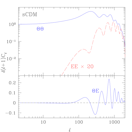
FIG. 6.: Power spectra for the standard cold dark matter model (scale invariant scalar adiabatic initial conditions with $\Omega_{0}=1$, $h=0.5$ and $\Omega_{B}h^{2}=0.0125$). Notice that $B$-polarization is absent, $E$-polarization scales as $\ell^{4}$ at large angles and the cross correlation ($\Theta E$) is negative at large angles and reflects the acoustic oscillations at small angles. In particular the phase of the $EE$ and $\Theta E$ acoustic peaks is set by the temperature oscillations $\Theta\Theta$ (see §IV B).

B Viscosity and Polarization

Anisotropic stress represents shear viscosity in the fluid and is generated as tight coupling breaks down on small scales where the photon diffusion length is comparable to the wavelength. For the photons, anisotropic stress is related to the quadrupole moments of the distribution $\Theta_{2}^{(m)}$ which is in turn coupled to the E-parity polarization $E_{2}^{(m)}$. The zeroth order expansion of the polarization $(\ell=2)$ equations (Eqn. 82) gives

$$E_{2}^{(m)}=-{\sqrt{6}\over 4}\Theta_{2}^{(m)},\qquad B_{2}^{(m)}=0$$ (119)

or $P^{(m)}={1\over 4}\Theta_{2}^{(m)}$. The quadrupole $(\ell=2)$ component of the temperature hierarchy (Eqn. 78) then becomes to lowest order in $k/\dot{\tau}$

$$\Theta_{2}^{(m)}={4\over 9}\sqrt{4-m^{2}}{k\over\dot{\tau}}\Theta_{1}^{(m)},\qquad P^{(m)}={1\over 9}\sqrt{4-m^{2}}{k\over\dot{\tau}}\Theta_{1}^{(m)}\,,$$ (120)

for scalars and vectors. In the tight coupling limit, the scalar and vector sources of polarization traces the structure of the photon-baryon fluid velocity. For the tensors,

$$\Theta_{2}^{(2)}=-{4\over 3}{\dot{H}\over\dot{\tau}}\,,\qquad P^{(2)}=-{1\over 3}{\dot{H}\over\dot{\tau}}\,.$$ (121)

Combining Eqns. (119) and (120), we see that polarization fluctuations are generally suppressed with respect to metric or temperature fluctuations. They are proportional to the quadrupole moments in the temperature which are suppressed by scattering. Only as the optical depth decreases can polarization be generated by scattering. Yet then the fraction of photons affected also decreases. In the standard cold dark matter model, the polarization is less than $5\%$ of the temperature anisotropy at its peak (see Fig. 6).

These scaling relations between the metric and anisotropic scattering sources of the temperature and polarization are important for understanding the large angle behavior of the polarization and temperature polarization cross spectrum. Here last scattering is effectively instantaneous compared with the scale of the perturbation and the tight coupling remains a good approximation through last scattering.

For the scalars, the Euler equation (110) may be used to express the scalar velocity and hence the polarization in terms of the effective temperature,

$$\Theta_{1}^{(0)}=m_{\rm eff}^{-1}\int k(\Theta_{0}^{(0)}+m_{\rm eff}\Psi)d\eta\,.$$ (122)

Since $m_{\rm eff}\sim 1$, $\Theta_{1}^{(0)}$ has the same sign as $\Theta_{0}^{(0)}+\Psi$ before $\Theta_{0}^{(0)}+\Psi$ itself can change signs, assuming reasonable initial conditions. It then follows that $P^{(0)}$ is also of the same sign and is of order

$$P^{(0)}\sim(k\eta){k\over\dot{\tau}}[\Theta_{0}^{(0)}+\Psi]\,,$$ (123)

which is strongly suppressed for $k\eta\ll 1$. The definite sign leads to a definite prediction for the sign of the temperature polarization cross correlation on large angles.

For the vectors

$$P^{(1)}={\sqrt{3}\over 9}{k\over\dot{\tau}}V\,,$$ (124)

and is both suppressed and has a definite sign in relation to the metric fluctuation. The tensor relation to the metric is given in Eqn. (121). In fact, in all three cases the dominant source of temperature perturbations has the same sign as the anisotropic scattering source $P^{(m)}$. From Eqn. (108), differences in the sense of the cross correlation between temperature and polarization thus arise only due to geometric reasons in the projection of the sources (see Fig. 5). On angles larger than the horizon at last scattering, the scalar and vector $C_{\ell}^{\Theta E}$ is negative whereas the tensor cross power is positive [9, 21].

On smaller scales, the scalar polarization follows the velocity in the tight coupling regime. It is instructive to recall the solutions for the acoustic oscillations from Eqn. (114). The velocity oscillates $\pi/2$ out of phase with the temperature and hence the $E$-polarization acoustic peaks will be out of phase with the temperature peaks (see Fig. 6). The cross correlation oscillates as $\cos(ks+\phi)\sin(ks+\phi)$ and hence has twice the frequency. Thus between peaks of the polarization and temperature power spectra (which represents both peaks and troughs of the temperature amplitude) the cross correlation peaks. The structure of the cross correlation can be used to measure the acoustic phase $\phi$ ($\phi\approx 0$ for adiabatic models) and how it changes with scale just as the temperature but like the $EE$ power spectrum [27] has the added benefit of probing slightly larger scales than the first temperature peak. This property can help distinguish adiabatic and isocurvature models due to causal constraints on the generation of acoustic waves at the horizon at last scattering [28].

Finally, polarization also increases the viscosity of the fluid by a factor of $6/5$, which has significant effects for the temperature. Even though the viscous imperfections of the fluid are small in the tight coupling region they can lead to significant dissipation of the fluctuations over time (see §IV D).

C Entropy and Heat Conduction

Differences in the bulk velocities of the photons and baryons $\Theta_{1}^{(m)}-v_{B}^{(m)}$ also represent imperfections in the fluid that lead to entropy generation and heat conduction. The baryon Euler equations (88) and (94) give

$$\Theta_{1}^{(0)}-v_{B}^{(0)} = {R\over\dot{\tau}}\left[\dot{v}_{B}^{(0)}+{\dot{a}\over a}v_{B}^{(0)}-k\Psi\right]\,,$$ (125)

$$\Theta_{1}^{(1)}-v_{B}^{(1)} = {R\over\dot{\tau}}\left[\dot{v}_{B}^{(1)}-\dot{V}+{\dot{a}\over a}(v_{B}^{(1)}-V)\right]\,,$$ (126)

which may be iterated to the desired order in $1/\dot{\tau}$. For scalar fluctuations, this slippage leads to the generation of non-adiabatic pressure or entropy fluctuations

$$\Gamma_{\gamma B} \equiv (\delta p_{\gamma B}-c_{\gamma B}^{2}\delta\rho_{\gamma B})/p_{\gamma B}$$ (127)

$$= -{4\over 3}{R\over 1+R}\int(\Theta_{1}^{(0)}-v_{B}^{(0)})k\,d\eta\,,$$ (128)

as the local number density of baryons to photons changes. Equivalently, this can be viewed as heat conduction in the fluid. For vorticity fluctuations, these processes do not occur since there are no density, pressure, or temperature differentials in the fluid.

D Dissipation

The generation of viscosity and heat conduction in the fluid dissipates fluctuations through the Euler equations with (120) and (126),

$$(1+R)\dot{\Theta}_{1}^{(0)} = k\left[\Theta_{0}^{(0)}+(1+R)\Psi\right]+{k\over\dot{\tau}}R^{2}\dot{\Theta}_{0}^{(0)}-{16\over 45}{k^{2}\over\dot{\tau}}\Theta_{1}^{(0)}\,,$$ (129)

$$(1+R)\dot{\Theta}_{1}^{(1)} = (1+R)\dot{V}-{k\over\dot{\tau}}{4\over 15}k\Theta_{1}^{(1)}\,,$$ (130)

where we have dropped the $\dot{a}/a$ factors under the assumption that the expansion can be neglected during the dissipation period. We have also employed Eqn. (116) to eliminate higher order terms in the vector equation. With the continuity equation for the scalars $\dot{\Theta}_{0}^{(0)}=-k\Theta_{1}^{(0)}/3-\dot{\Phi}$ (see Eqn. 78 $\ell=0$, $m=0$ ), we obtain

$$\ddot{\Theta}_{0}^{(0)}+{1\over 3}{k^{2}\over\dot{\tau}}\left[{R^{2}\over(1+R)^{2}}+{16\over 15}{1\over 1+R}\right]\dot{\Theta}_{0}^{(0)}+{k^{2}\over 3(1+R)}\Theta_{0}^{(0)}=-{k^{3}\over 3}\Psi-\ddot{\Phi}\,,$$ (131)

which is a damped forced oscillator equation.

An interesting case to consider is the behavior in the absence of metric fluctuations $\Psi$, $\Phi$, and $V$. The result, immediately apparent from Eqn. (130) and (131), is that the acoustic amplitude $(m=0)$ and vorticity $(m=1)$ damp as $\exp[-(k/k_{D}^{(m)})^{2}]$ where

$$\left[{1\over k_{D}^{(0)}}\right]^{2} = {1\over 6}\int d\eta\,{1\over\dot{\tau}}{{R^{2}+16(1+R)/15}\over{(1+R)^{2}}}\,,$$ (132)

$$\left[{1\over k_{D}^{(1)}}\right]^{2} = {4\over 15}\int d\eta{1\over\dot{\tau}}{1\over{1+R}}\,.$$ (133)

Notice that dissipation is less rapid for the vectors compared with the scalars once the fluid becomes baryon dominated $R\gg 1$ because of the absence of heat conduction damping. In principle, this allows vectors to contribute more CMB anisotropies at small scales due to fluid contributions. In practice, the dissipative cut off scales are not very far apart since $R\lesssim 1$ at recombination.

Vectors may also dominate if there is a continual metric source. There is a competition between the metric source and dissipational sinks in Eqns. (130) and (131). Scalars retain contributions to $\Theta^{(0)}_{0}+\Psi$ of ${\cal O}(R\Psi,(\ddot{\Psi}-\ddot{\Phi})/k^{2})$ (see Eqn. (115) and [29]). The vector solution becomes

$$\Theta_{1}^{(1)}(\eta)=e^{-[k/k_{D}^{(1)}(\eta)]^{2}}\int_{0}^{\eta}d\eta^{\prime}\dot{V}e^{[k/{k_{D}^{(1)}}(\eta^{\prime})]^{2}},$$ (134)

which says that if variations in the metric are rapid compared with the damping then $\Theta_{1}^{(1)}=V$ and damping does not occur.

V Scaling Stress Seeds

Stress seeds provide an interesting example of the processes considered above by which scalar, vector, and tensor metric perturbations are generated and affect the temperature and polarization of the CMB. They are also the means by which cosmological defect models form structure in the universe. As part of the class of isocurvature models, all metric fluctuations, including the (scalar) curvature perturbation are absent in the initial conditions. To explore the basic properties of these processes, we employ simple examples of stress seeds under the restrictions they are causal and scale with the horizon length. Realistic defect models may be constructed by superimposing such simple sources in principle.

We begin by discussing the form of the stress seeds themselves (§V A) and then trace the processes by which they form metric perturbations (§V B) and hence CMB anisotropies (§V C).

A Causal Anisotropic Stress

Stress perturbations are fundamental to seeded models of structure formation because causality combined with energy-momentum conservation forbids perturbations in the energy or momentum density until matter has had the opportunity to move around inside the horizon (see e.g. [30]). Isotropic stress, or pressure, only arises for scalar perturbations and have been considered in detail by [27]. Anisotropic stress perturbations can also come in vector and tensor types and it is their effect that we wish to study here. Combined they cover the full range of possibilities available to causally seeded models such as defects.

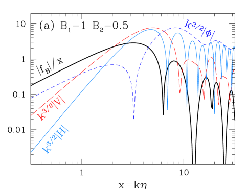
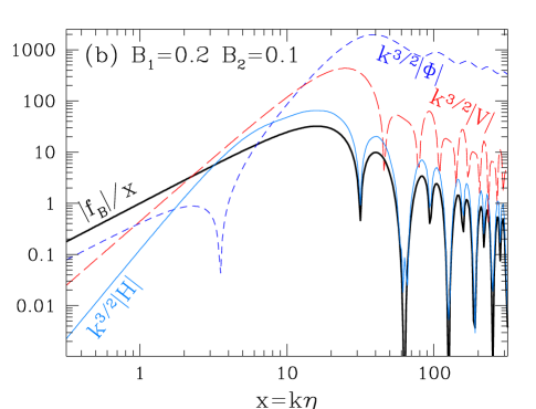
FIG. 7.: Metric fluctuations from scaling anisotropic stress seeds sources. The same anisotropic stress seed (bold solid lines $a^{2}\pi_{s}\propto f_{B}/x$) produce qualitatively different scalar (short-dashed), vector (long-dashed), and tensor (solid) metric perturbations. As discussed in the text the behavior scales with the characteristic time of the source $x_{c}\propto B_{1}^{-1}$. The left panel (a) shows a source which begins to decay as soon as causally permitted ($B_{1}=1$) and the right panel (b) the effect of delaying the decay ($B_{1}=0.2$). We have displayed the results here for a photon-dominated universe for simplicity.

We impose two constraints on the anisotropic stress seeds: causality and scaling. Causality implies that correlations in the stresses must vanish outside the horizon. Anisotropic stresses represent spatial derivatives of the momentum density and hence vanish as $k^{2}$ for $k\eta\ll 1$. Scaling requires that the fundamental scale is set by the current horizon so that evolutionary effects are a function of $x=k\eta$. A convenient form that satisfies these criteria is [27, 31]

$$4\pi Ga^{2}\pi_{s}^{(m)}=A^{(m)}\eta^{-1/2}f_{B}(x)\,,$$ (135)

with

$$f_{B}(x)={6\over B_{2}^{2}-B_{1}^{2}}\left[{\sin(B_{1}x)\over(B_{1}x)}-{\sin(B_{2}x)\over(B_{2}x)}\right]\,,$$ (136)

with $0<(B_{1},B_{2})<1$. We caution the reader that though convenient and complete, this choice of basis is not optimal for representing the currently popular set of defect models. It suffices for our purposes here since we only wish to illustrate general properties of the anisotropy formation process.

Assuming $B_{1}>B_{2}$, $B_{1}$ controls the characteristic time after horizon crossing that the stresses are generated, i.e. the peak in $f_{B}$ scales as $k\eta_{c}\equiv x_{c}\propto B_{1}^{-1}$ (see Fig. 7). $B_{2}$ controls the rate of decline of the source at late times. In the general case, the seed may be a sum of different pairs of $(B_{1},B_{2})$ which may also differ between scalar, vector, and tensor components.

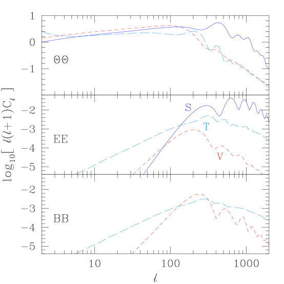
FIG. 8.: Temperature and polarization power spectra for a scaling anisotropic stress seeds with the minimal characteristic time $B_{1}=1$ for scalars (S, solid), vectors (V, short-dashed), and tensors (T, long-dashed). Scalar temperature fluctuations at intermediate scales are dominated by acoustic contributions which then damp at small scales. $B$-parity polarization contributions are absent for the scalars, larger by an order of magnitude than $E$-parity contributions for the vectors and similar to but smaller than the $E$-parity for the tensors. Features in the vector and tensor spectra are artifacts of our choice of source and are unlikely to be present in a realistic model. The background cosmology is set to $\Omega_{0}=1$, $h=0.5$, $\Omega_{B}h^{2}=0.0125$.

B Metric Fluctuations

Let us consider how the anisotropic stress seed sources generate scalar, vector and tensor metric fluctuations. The form of Eqn. (136) implies that the metric perturbations also scale so that $k^{3}|h|^{2}=f(x=k\eta)$ where $f$ may be different functions for $h=(\Psi,\Phi,V,H)$. Thus scaling in the defect field also implies scaling for the metric evolution and consequently the purely gravitational effects in the CMB as we shall see in the next section. Scattering introduces another fundamental scale, the horizon at last scattering $\eta_{*}$, which we shall see breaks the scaling in the CMB.

It is interesting to consider differences in the evolutions for the same anisotropic stress seed, $A^{(m)}=1$ with $B_{1}$ and $B_{2}$ set equal for the scalars, vectors and tensors. The basic tendencies can be seen by considering the behavior at early times $x\lesssim x_{c}$. If $x\ll 1$ as well, then the contributions to the metric fluctuations scale as

$$k^{3/2}\Phi/f_{B}={\cal O}(x^{-1})\,,\qquad \qquad k^{3/2}\Psi/f_{B}={\cal O}(x^{-1})\,,$$ (137)

$$k^{3/2}V/f_{B}={\cal O}(x^{0})\,,\qquad \qquad k^{3/2}H/f_{B}={\cal O}(x^{1})\,,$$ (138)

where $f_{B}=x^{2}$ for $x\ll 1$. Note that the sources of the scalar fluctuations in this limit are the anisotropic stress and momentum density rather than energy density (see Eqn. 83). This behavior is displayed in Fig. 7(a). For the scalar and tensor evolution, the horizon scale enters in separately from the characteristic time $x_{c}$. For the scalars, the stresses move matter around and generate density fluctuations as $\rho_{s}\sim x^{2}\pi_{s}$. The result is that the evolution of $\Psi$ and $\Phi$ steepens by $x^{2}$ between $1\lesssim x\lesssim x_{c}$. For the tensors, the equation of motion takes the form of a damped driven oscillator and whose amplitude follows the source. Thus the tensor scaling becomes shallower in this regime. For $x\gtrsim x_{c}$ both the source and the metric fluctuations decay. Thus the maximum metric fluctuation scales as

$$k^{3/2}\Phi/f_{B}(x_{c})={\cal O}(x_{c}^{1})\,,\qquad \qquad k^{3/2}\Psi/f_{B}(x_{c})={\cal O}(x_{c}^{1})\,,$$ (139)

$$k^{3/2}V/f_{B}(x_{c})={\cal O}(x_{c}^{0})\,,\qquad \qquad k^{3/2}H/f_{B}(x_{c})={\cal O}(x_{c}^{-1}).$$ (140)

For a late characteristic time $x_{c}>1$, fluctuations in the scalars are larger than vectors or tensors for the same source (see Fig. 7b). The ratio of acoustic to gravitational redshift contributions from the scalars scale as $x_{c}^{-2}$ by virtue of pressure support in Eqn. (115) and thus acoustic oscillations become subdominant as $B_{1}$ decreases.

C CMB Anisotropies

Anisotropy and structure formation in causally seeded, or in fact any isocurvature model, proceeds by a qualitatively different route than the conventional adiabatic inflationary picture. As we have seen, fluctuations in the metric are only generated inside the horizon rather than at the initial conditions (see §V B). Since CMB anisotropies probe scales outside the horizon at last scattering, one would hope that this striking difference can be seen in the CMB. Unfortunately, gravitational redshifts between last scattering and today masks the signature in the temperature anisotropy. The scaling ansatz for the sources described in §V A in fact leads to near scale invariance in the large angle temperature because fluctuations are stimulated in the same way for each $k$-mode as it crosses the horizon between last scattering and the present. While these models generically leave a different signature in modes which cross the horizon before last scattering [22, 27], models which mimic adiabatic inflationary predictions can be constructed [31].

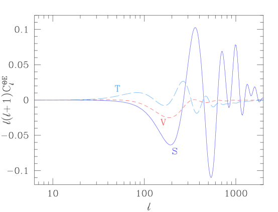
FIG. 9.: Temperature-polarization cross power spectrum for the model of Fig. 8. Independent of the nature of the sources, the cross power at angles larger than that subtended by the horizon at last scattering is negative for the scalars and vectors and positive for the tensors. The more complex structure for the scalars at small angular scales reflects the correlation between the acoustic effective temperature and velocity at last scattering.

Polarization provides a more direct test in that it can only be generated through scattering. The large angle polarization reflects fluctuations near the horizon at last scattering and so may provide a direct window on such causal, non-inflationary models of structure formation. One must be careful however to separate scalar, vector and tensor modes whose different large angle behaviors may obscure the issue. Let us now illustrate these considerations with the specific examples introduced in the last section.

The metric fluctuations produced by the seed sources generate CMB anisotropies through the Boltzmann equation (78). We display an example with $B_{1}=1$ and $B_{2}=0.5$ in Fig. 8. Notice that scaling in the sources does indeed lead to near scale invariance in the large angle temperature but not the large angle polarization. The small rise toward the quadrupole for the tensor temperature is due to the contribution of long-wavelength gravity waves that are currently being generated and depends on how rapidly they are generated after horizon crossing. Inside the horizon at last scattering (here $\ell\gtrsim 200$), scalar fluctuations generate acoustic waves as discussed in §IV which dominate for small characteristic times $x_{c}\approx 1$. On the other hand, these contributions are strongly damped below the thickness of the last scattering surface by dissipational processes. Note that features in the vector and tensor spectrum shown here are artifacts of our choice of source function. In a realistic model, the superposition of many sources of this type will wash out such features. The general tendencies however do not depend on the detailed form of the source. Note that vector and tensor contributions damp more slowly and hence may contribute significantly to the small-angle temperature anisotropy.

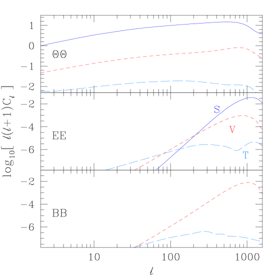
FIG. 10.: Same as Fig. 8 except with a larger characteristic time $B_{1}=0.2$, $B_{2}=0.1$. Scalar gravitational redshift effects now dominate over scalar acoustic as well as vector and tensor contributions for the same stress source due the process by which stress perturbations generate metric fluctuations (see Fig. 7).

Polarization can only be generated by scattering of a quadrupole temperature anisotropy. For seeded models, scales outside the horizon at last scattering $k\eta_{*}\lesssim 1$ have not formed significant metric fluctuations (see e.g. Fig. 7). Hence quadrupole fluctuations, generated from the metric fluctuations through Eqns. (121), (123), and (124), are also suppressed. The power in $k$ of the polarization thus drops sharply below $k\eta_{*}=1$. This drop of course corresponds to a lack of large angle power in the polarization. However its form at low $\ell$ depends on geometric aspects of the projection from $k$ to $\ell$. In these models, the large angle polarization is dominated by projection aliasing of power from small scales $k\eta_{*}\gtrsim 1$. The asymptotic expressions of Eqn. (102) thus determine the large angle behavior of the polarization: $\ell^{2}C_{\ell}\propto\ell^{6}$ for scalars $(EE)$, $\ell^{4}$ for vectors and $\ell^{2}$ for tensors ($EE$ and $BB$); the cross spectrum $(\Theta E)$ goes as $\ell^{4}$ for each contribution. For comparison, the scale invariant adiabatic inflationary prediction has scalar polarization ($EE$) dropping off as $\ell^{4}$ and cross spectrum ($\Theta E$) as $\ell^{2}$ from Eqn. (123) because of the constant potential above the horizon (see Fig. 6). Seeded models thus predict a more rapid reduction in the scalar polarization for the same background cosmology.

Polarization can also help separate the three types of fluctuations. In accord with the general prediction (see §III D), scalars produce no $B$-parity polarization, whereas vector $B$-parity dominates $E$-parity polarization by a factor of $6$ and tensor $B$-parity is suppressed by a factor of $8/13$ (see Eqn. (37)). Differences also arise in the temperature-polarization cross power spectra $C_{\ell}^{\Theta E}$ shown in Fig. 9. Independent of the nature of the source, above the angle the horizon subtends at last scattering, scalar and vector temperature perturbations from the last scattering surface [21] are anticorrelated with polarization, whereas they are correlated for tensor perturbations (see §IV B and [9]). Inside the horizon, the scalar polarization follows the scalar velocity which is $\pi/2$ out of phase with the effective temperature (see Eqn. 120). In the adiabatic model, scalar cross correlation reverses signs before the first acoustic peak, as compression overcomes the gravitational redshift of the Sachs-Wolfe effect, unlike the isocurvature models (see Fig. 6 and [28]). The sign test to distinguish scalars from tensors must thus be performed on scales larger than twice the first peak. Conversely, to use the cross correlation to distinguish adiabatic from isocurvature fluctuations, the scalar and tensor contributions must be separated.

How do these results change with the model for the seeds? As we increase the characteristic time $x_{c}$ by decreasing $B_{1}=0.2$, the main effect comes from differences in the generation of metric fluctuations discussed in §V B. For the same amplitude anisotropic stress, scalars contributions dominate the vector and tensor contributions by factors of $x_{c}=B_{1}^{-1}$ (see Eqn. 140). Note however that the scalar contributions come from the gravitational redshifts between last scattering and today rather than the acoustic oscillations (see §IV A) and hence produce no strong features. Because of the late generation of metric fluctuations in these models, the peak in the polarization spectra is also shifted with $x_{c}$. Note however that the qualitative behavior of the polarization described above remains the same.

Although these examples do not exhaust the full range of possibilities for scaling seeded models, the general behavior is representative. Equal amplitude anisotropic stress sources tend to produce similar large angle temperature anisotropies if the source is active as soon as causally allowed $x_{c}\approx 1$. Large angle scalar polarization is reduced as compared with adiabatic inflationary models because of causal constraints on their formation. This behavior is not as marked in vectors and tensors due to the projection geometry but the relative amplitudes of the $E$-parity and $B$-parity polarization as well as the $\Theta E$ cross correlation can be used to separate them independently of assumptions for the seed sources. Of course in practice these tests at large angles will be difficult to apply due to the smallness of the expected signal.

Reionization increases the large angle polarization signal because the quadrupole anisotropies that generate it can be much larger [32]. This occurs since decoupling occurs gradually and the scattering is no longer rapid enough to suppress anisotropies. The prospects for separating the scalars, vectors and tensors based on polarization consequently also improve [33].

For angles smaller than that subtended by the horizon at last scattering, the relative contributions of these effects depends on a competition between scalar gravitational and acoustic effects and the differences in the generation and damping behavior of the scalar, vector and tensor perturbations.

VI Discussion

We have provided a new technique for the study of temperature and polarization anisotropy formation in the CMB which introduces a simple and systematic representation for their angular distributions. The main virtue of this approach is that the gravitational and scattering sources are directly related to observable properties in the CMB. One can then explore properties that are independent of the source, which tell us the broad framework, e.g. the classical cosmological parameters and the nature of fluctuations in the early universe, and identify properties that are dependent on the source, which can help pin down the model for structure formation. An example of the former is the fact that scalar fluctuations generate no magnetic parity polarization [3, 4], vectors generate mainly magnetic parity polarization, and tensors generate comparable but somewhat smaller magnetic parity polarization. Large angle polarization of the three components are also constrained by model-independent geometric arguments in its slope and its correlation with the temperature anisotropy. If the scalar contributions can be isolated from the vectors, tensors and other foreground sources of polarization from these and other means, these constraints translate into a robust distinction between isocurvature and adiabatic models for structure formation.

In our representation, the temperature and polarization distributions are projections on the sky of four simple sources, the metric fluctuation (via the gravitational redshift), the intrinsic temperature at last scattering, the baryon velocity at last scattering (via the Doppler effect) and the temperature and polarization quadrupoles at last scattering (via the angular dependence of Compton scattering). As such, it better reveals the power of the CMB to probe the nature of these sources and extract information on the process of structure formation in the universe. As an example, we have explored how general properties of scaling stress seeds found in cosmological defect models manifest themselves in the temperature and polarization power spectra. The framework we have provided here should be useful for determining the robust signatures of specific models for structure formation as well as the reconstruction of the true model for structure formation from the data as it becomes available.

Acknowledgements: We would like to thank Uros Seljak and Matias Zaldarriaga for many useful discussions. W.H. was supported by the W.M. Keck Foundation.

TAB-2. Commonly used symbols. $m=0,\pm 1,\pm 2$ for the scalars, vectors, and tensors. For the fluid variables $f\rightarrow\gamma$ for the photons, $f\rightarrow B$ for the baryons and $\gamma B$ for the photon-baryon fluid. $X=\Theta$, $E$, $B$ for the temperature-polarization power spectra.

Symbol	Definition	Eqn.
$\Psi,\Phi$	Scalar metric	(51)
$\Theta_{\ell}^{(m)}$	$\Delta T/T$ moments	(73)
$\alpha,\beta,\gamma$	Euler angles	(13)
$\beta^{(m)}_{\ell},\epsilon^{(m)}_{\ell}$	Radial $B,E$ function	(24)
$\delta_{f}$	Fluid density perturbation	(54)
$\eta$	Conformal time	(50)
$\,{}_{s}^{\vphantom{m}}\kappa_{\ell}^{m}$	Clebsch-Gordan coefficient	(77)
$\rho_{f},\rho_{s}$	Fluid, seed density	(54)
$\pi_{f}^{(m)},\pi_{f}^{(m)}$	Fluid, seed anisotropic stress	(54)
$\theta,\phi$	Spherical coordinates in $\hat{k}$ frame	(17)
$\tau$	Thomson optical depth	(64)
$B_{\ell}^{(m)}$	$B$-pol. moments	(73)
$\vec{C}$	Collision term	(65)
${C_{\ell}^{X\widetilde{X}(m)}}$	$X\widetilde{X}$ power spectrum from $m$	(74)
$E_{\ell}^{(m)}$	$E$-pol. moments	(73)
$\vec{G}$	Gravitational redshift term	(72)
$G_{\ell}^{m}$	Temperature basis	(17)
${}_{\pm 2}^{\vphantom{2}}G_{\ell}^{m}$	Polarization basis	(18)
$H$	Tensor metric	(53)

Symbol	Definition	Eqn.
${\bf M}_{\pm}$	(Pauli) matrix basis	(1)
$P^{(m)}$	Anisotropic scattering source	(80)
$Q^{(0)}$	Scalar basis	(41)
$Q^{(1)}_{i}$	Vector basis	(43)
$Q^{(2)}_{ij}$	Tensor basis	(47)
$R$	$B/\gamma$ momentum density	(86)
$S_{\ell}^{(m)}$	Temperature source	(79)
$V$	Vector metric	(52)
$\,{}_{s}^{\vphantom{m}}Y_{\ell}^{m}$	Spin-$s$ harmonics	(8)
$j_{\ell}^{(\ell^{\prime}m)}$	Radial temp function	(23)
$\vec{k}$	Wavenumber	(17)
$k_{D}^{(m)}$	Damping wavenumber	(133)
$\ell$	Multipole	(8)
$m_{\rm eff}$	Effective mass $1+R$	(110)
$\hat{n}$	Propagation direction	(19)
$p_{f},p_{s}$	Fluid, seed pressure	(54)
$v_{f}^{(m)}$	Fluid velocity	(54)
$v_{s}^{(m)}$	Seed momentum density	(54)
$w_{f}$	$p_{f}/\rho_{f}$	(85)

Published in: Physical Review D 56, 596 (1997)

whu@ias.edu

http://www.sns.ias.edu/$\sim$whu

http://www.sns.ias.edu/$\sim$whu/polar/polar.html and astro-ph/9706147 for a descriptive accounts of this work.

REFERENCES

- [1] MAP: http://map.gsfc.nasa.gov
- [2] Planck Surveyor: http://astro.estec.esa.nl/SA-general/Projects/Cobras/cobras.html
- [3] U. Seljak & M. Zaldarriaga, Phys. Rev. Lett. 78, 2054 (1997) [astro-ph/9609196]; M. Zaldarriaga & U. Seljak, Phys. Rev. D 55, 1830 (1997) [astro-ph/9609170]
- [4] M. Kamionkowski, A. Kosowsky, & A. Stebbins, Phys. Rev. Lett. 78, 2058 (1997) [astro-ph/9609132]; ibid, Phys. Rev. D. 55, 7368 (1997) [astro-ph/9611125]
- [5] W. Hu & M. White, Astrophys. J. Lett. (in press) [astro-ph/9701219]
- [6] K. Tomita, Prog. Theor. Phys. 68, 310 (1982)
- [7] L.F. Abbott & R.K. Schaeffer, Astrophys. J. 308, 546 (1986)
- [8] W. Hu, U. Seljak, M. White, & M. Zaldarriaga (in preparation)
- [9] R.G. Crittenden, D. Coulson, & N.G. Turok, Phys. Rev. D 52, 5402 (1995) [astro-ph/9411107]; R.G. Crittenden, R.L. Davis, P.J. Steinhardt, Astrophys. J. Lett 417, L13 (1993) [astro-ph/9306027]
- [10] A.G. Polnarev, Sov. Astron. 29, 607 (1985)
- [11] J.R. Bond & G. Efstathiou, Astrophys. J. Lett. 285, L45 (1984); ibid. Mon. Not. Roy. Astr. Soc. 226, 655 (1987)
- [12] E. Newman & R. Penrose, J. Math Phys 7, 863 (1966); J.N. Goldberg et al., J. Math Phys. 8, 2155 (1967); K.S. Thorne, Rev. Mod. Phys. 52, 299 (1980).
- [13] J.J. Sakurai, Modern Quantum Mechanics (Addison-Wesley, New York, 1985) p. 215
- [14] J.D. Jackson, Classical Electrodynamics (Wiley, New York 1972)
- [15] H. Kodama & M. Sasaki, Prog. Theor. Phys. 78, 1 (1984)
- [16] S. Chandrasekhar, Radiative Transfer (Dover, New York, 1960)
- [17] J.M. Bardeen, Phys. Rev. D22, 1882 (1980)
- [18] R. Durrer, Phys. Rev. D42, 2533 (1990)
- [19] A. Kosowsky, Ann. Phys. 246, 49 (1996) [astro-ph/9501045]; A. Melchiorri & N. Vittorio, preprint, astro-ph/9610029.
- [20] R.K. Sachs & A.M. Wolfe, Astrophys. J. 147, 73 (1967)
- [21] There can be a small contribution from unequal time correlations at the very lowest if the main signal from the last scattering surface is falling sufficiently rapidly.
- [22] W. Hu & N. Sugiyama, Astrophys. J. 444, 489 (1995) [astro-ph/9406071]; ibid, Phys. Rev. D51, 2599 (1995) [astro-ph/9411008].
- [23] M. Zaldarriaga & D. Harari, Phys. Rev. D55, 3276 (1995) [astro-ph/9504085]
- [24] U. Seljak & M. Zaldarriaga, Astrophys. J. 469, 437 (1996) [astro-ph/9603033]
- [25] P.J.E. Peebles & J.T. Yu, Astrophys. J. 162, 815 (1970)
- [26] N. Kaiser, Mon. Not. Roy. Astron. Soc. 202, 1169 (1983)
- [27] W. Hu, D.N. Spergel, & M. White, Phys. Rev. D 55, 3288 (1997) [astro-ph/9605193]
- [28] D.N. Spergel & M. Zaldarriaga preprint, astro-ph/9705182; R. Battye & D. Harrari (in preparation)
- [29] W. Hu & M. White, Astrophys. J. 479, 568 (1997) [astro-ph/9609079]; R. Battye, Phys. Rev. D 55, 7361 [astro-ph/9610197]
- [30] S. Veeraraghavan & A. Stebbins, Astrophys. J. 365, 37 (1990)
- [31] N. Turok, Phys. Rev. D. 54, 3686 (1996) [astro-ph/9604172]; ibid Phys. Rev. Lett. 77, 4138 (1996) [astro-ph/9607109].
- [32] J. Negroponte & J. Silk, Phys. Rev. Lett. 44, 1433 (1980); M.M. Basko & A.G. Polnarev Mon. Not. Roy. Astr. Soc. 191, 207 (1980); C.J. Hogan, N. Kaiser, M. Rees, Philos. Trans. Roy. Soc. London Series A 307, 97 (1982)
- [33] M. Zaldarriaga, D.N. Spergel, U. Seljak, preprint, astro-ph/9702157