On Measuring Nebular Chemical Abundances in Distant Galaxies Using Global Emission Line Spectra

Abstract

The advent of 8–10 meter class telescopes enables direct measurement of the chemical properties in the ionized gas of cosmologically–distant galaxies with the same nebular analysis techniques used in local H II regions. We show that spatially unresolved (i.e., global) emission line spectra can reliably indicate the chemical properties of distant star-forming galaxies. However, standard nebular chemical abundance measurement methods (those with a measured electron temperature from [O III] $\lambda$4363) may be subject to small systematic errors when the observed volume includes a mixture of gas with diverse temperatures, ionization parameters, and metallicities. To characterize these systematic effects, we compare physical conditions derived from spectroscopy of individual H II regions with results from global galaxy spectroscopy. We consider both low-mass, metal poor galaxies with uniform abundances and larger galaxies with internal chemical gradients. For low-mass galaxies, standard chemical analyses using global spectra produce small systematic errors in that the derived electron temperatures are 1000 K — 3000 K too high due to non-uniform electron temperatures and large variations in ionization parameter. As a result, the oxygen abundances derived from direct measurements of the electron temperatures are too low, but it is possible to compensate for this effect by applying a correction of $\Delta(O/H)=+0.1$ dex to the oxygen abundances derived from global spectra. For more massive metal-rich galaxies like local spirals, direct measurements of electron temperatures are seldom possible from global spectra. Well-established empirical calibrations using strong-line ratios can serve as reliable ($\pm$0.2 dex) indicators of the overall systemic oxygen abundance even when the signal-to-noise of the $H\beta$ and [O III] emission lines is as low as 8:1. We present prescriptions, directed toward high-redshift observers, for using global emission line spectra to trace the chemical properties of star-forming galaxies in the distant universe.

1 Using Integrated Galaxy Spectra as Chemical Diagnostics

Optical emission lines from H II regions have long been the primary means of gas-phase chemical diagnosis in galaxies (Aller 1942; Searle 1971; reviews by Peimbert 1975; Pagel 1986; Shields 1990; Aller 1990). With the advent of large telescopes and sensitive spectrographs, nebular emission lines from distant star-forming regions can probe the chemical evolution of objects at earlier epochs (Steidel et al. 1996; Kobulnicky & Zaritsky 1998) in a complementary manner to absorption line measurements (reviewed by Lauroesch et al. 1996). Optical emission line spectroscopy preferentially samples the warm ionized phase of the interstellar medium in the immediate vicinity of recent star formation events (i.e., H II regions). Madau et al. (1996), Lilly et al. (1996) observe that the rate of star-forming is higher in the past, so potential emission line targets are plentiful at redshifts of $0.3<z<2$. Compared to absorption-line studies which are limited to lines of sight toward bright background quasars, nebular emission line observations are possible in any galaxy with H II regions. Complications due to line width ambiguities, saturation effects, multiple velocity components, and ionization corrections are less severe or absent for nebular spectroscopy. Limited signal-to-noise and lack of spatial resolution are the two most formidable obstacles for ground-based spectroscopic studies of cosmologically distant H II regions. A typical ground-based resolution element of 1.0^′′ corresponding to a linear size of 5.2 kpc at $z=0.5$ will encompass entire galaxies. Our motivation in this paper is to explore the utility of spatially-integrated emission line spectroscopy for studying the chemical properties of star-forming galaxies at earlier epochs.

Osterbrock (1989) thoroughly discusses the standard techniques for measuring the chemical properties of ionized gas. Typically, chemical analyses of H II regions require measurement of H and He recombination lines along with collisionally-excited lines from one or more ionization states of heavy element species. Oxygen is the most commonly–used metallicity indicator in the ISM by virtue of its high relative abundance and strong emission lines in the optical part of the spectrum (e.g., [O II] $\lambda$3727 and [O III] $\lambda\lambda$4959,5007). In best-case scenarios, the electron temperature of the ionized medium can be derived from the ratio of a higher-excitation auroral line, such as [O III] $\lambda$4363, to [O III] $\lambda$5007. In practice, [O III] $\lambda$4363 is difficult to measure since it is typically only a few percent the strength of H$\beta$ even in the most metal-poor H II regions (I Zw 18; (O/H)=0.02(O/H)_⊙), and becomes unmeasurably weak in more metal-rich environments. The electron density of the medium may also be constrained using the density-sensitive ratio of [S II] $\lambda$6713/[S II] $\lambda$6731 or [O II] $\lambda$3727/[O II] $\lambda$3729 doublets. When bright H II regions are available, abundances of He, C, Ne, Si, S, and Ar are well-measured in many local galaxies. However, in cosmologically distant H II regions, only the brightest lines may be detectable, even using the collecting area and sensitivity of the largest telescope/instrument combinations envisioned today. A typical ground-based resolution element will encompass large fractions of galaxies exhibiting a wide variety of physical characteristics. Are global galaxy spectra in any way indicative of the physical properties of its ISM?

Three effects may bias spatially-integrated (global) emission line spectra of galaxies (kpc–sized apertures) compared to the values that would be derived from individual H II regions observed with higher spatial resolution (10—100 pc–sized apertures).

1) The aperture may include a mixture of gas or multiple H II regions with similar metallicity but differing ionization conditions.

2) The aperture may include a mixture of gas or multiple H II regions with significantly different metallicities.

3) The aperture may include a mixture of overlapping stellar absorption and nebular emission features which adversely affect the measured equivalent widths and emission line strengths.

One or several of these effects may reduce the precision of chemical abundance determinations using global galaxy spectra. In this paper, we explore the magnitude of such effects by comparing chemical analyses based upon local and global spectroscopy of nearby, well-studied galaxies. In Section 2 we consider the case of dwarf galaxies with uniform gas-phase abundance distributions, but a range of ionization conditions. In Section 3, we consider larger spiral galaxies which exhibit both chemical abundance and ionization variations. In Section 4 we consider the case of low-S/N spectra in which emission line strengths may be affected by underlying stellar absorption. We also consider the possibility of measuring oxygen abundances when only the H$\beta$ and [O III] emission lines are detected. The summary in Section 5 recaps the prospects for using global galaxy spectroscopy to study the chemical properties of star-forming objects in the early universe. Note of Caution: The prescriptions for deriving gas-phase metal abundances provided here assume that the nebular emission line spectrum is generated by photoionization from massive stars. Non-stellar ionizing sources, such as AGN, can generate emission spectra that superficially resemble photoionized H II regions. Generally, non-stellar energy sources produce distinctive emission line ratios compared to ordinary H II regions. Veilleux & Osterbrock (1987) and Heckman (1980) provide diagnostic diagrams which should be consulted to ascertain that ionizing sources are stellar in nature before proceeding with chemical analysis.

2 The Case of Metal-Poor Irregular and Dwarf Galaxies

Low-mass galaxies with sizes and luminosities smaller than that of the LMC appear to be chemically homogeneous on scales from $\sim$10 pc to 1 kpc (review by Kobulnicky 1998). Yet, they often contain a multiplicity of H II regions, and they exhibit a variety of ionization conditions. Localized high surface–brightness, high-ionization H II regions lie amidst a network of extended low-ionization filaments which sometimes stretch for a kpc or more (e.g., Hunter 1994; Hunter & Gallagher 1997). What is the effect of mixing these regions of disparate ionization parameter into a single aperture? We address this question empirically by considering both spatially integrated and localized measurements of ionized gas in a sample of nearby irregular galaxies.

2.1 Data Collection

We obtained new spectroscopic observations of the irregular and blue compact galaxies NGC 3125 ($\equiv$Tololo 1004-296), NGC 5253, Henize 2-10, Tololo 35 ($\equiv$Tololo 1324-276$\equiv$IC4249) on 4-6 February 1998 using the 4 m telescope + RC spectrograph at the Cerro Tololo InterAmerican Observatory. The KPGL-3 grating produced a dispersion of 1.2 Å pixel^-1 across the wavelength range 3700Å – 7000 Å imaged onto the 1k x 3k Loral CCD. A slit width of 2^′′ produced a spectral resolution of 5.1 Å. Seeing averaged 1-2^′′ through occasional light cirrus clouds and airmasses ranged from 1.0 to 1.6. The spatial scale of the CCD was 0.50^′′ pixel ^-1. The data were reduced in the standard fashion, by subtracting overscan bias, and dividing by a flat field image produced from a combination of dome-illuminated exposures and exposures of a quartz continuum lamp inside the spectrograph. Based on exposures of the twilight sky, we applied to the data a correction for variations in the illumination pattern along the 5^′ slit length. This combination of dome and internal lamp flats was necessary to achieve good S/N over the full wavelength range, and to correct for scattered light within the instrument during quartz lamp exposures. Periodic exposures of HeAr arc lamps allowed a wavelength solution accurate to $\sim$0.5 Å rms. Multiple observations of the standard stars GD108, GD50, Hz4, and SA95-42 (Oke 1990) with a slit width of 6^′′ over a range of airmass provided a site-dependent atmospheric extinction curve which we found to be consistent with the mean CTIO extinction curve. Standard star exposures also allowed us to derive the instrumental sensitivity function which had a pixel-to-pixel RMS of 2%. Between five and twenty 6-pixel apertures were defined across the nebular portion of each galaxy. We extracted multiple one-dimensional spectra of each object with aperture sizes of 6 pixels which correspond to linear sizes of 20 pc to 100 pc at the distances of the galaxies. We used emission-free regions 20-pixels or larger on either side of the aperture to define the mean background sky level which was subtracted from the source spectrum.

In order to measure a global emission line spectrum, we performed 5 and 10-minute drift scans of each galaxy by moving the telescope at a rate of 1^′′ $s^{-1}$ back and forth across the galaxy perpendicular to the slit. Summing the spatial extent of the nebular emission (100–300 pixels), we produced a global spectrum of the galaxy at the same spectral resolution as the fixed-pointing exposures. Figure 1 displays the global spectrum for each galaxy in arbitrary units. For display purposes, we plot each spectrum a second time, multiplied by a factor of 40.

To augment the sample, we selected four additional irregular galaxies with both global and local nebular spectroscopy in the literature. Kennicutt (1992—K92) presents spatially-integrated spectra for NGC 1569, NGC 4449, and NGC 4861$\equiv$Mrk 59. We used nebular spectroscopy of individual H II regions for these galaxies from Kobulnicky & Skillman (1997—NGC 1569), Talent (1980—NGC 4449), and our own 3.5 m Calar Alto spectra (Kobulnicky, in prep—NGC 4861; observations as described in Skillman, Bowmans & Kobulnicky 1997). Using the longslit data described in Kobulnicky & Skillman (1996), we constructed a global spectrum for NGC 4214.

We analyzed the one-dimensional localized spectra and global spectra for each galaxy using the nebular emission–line software and procedures described in Kobulnicky & Skillman (1996). The flux in each emission line was measured with single Gaussian fits. In the case of blended lines or lines with low-S/N, we fixed the width and position of the fit using the width and position of other strong lines nearby. Logarithmic extinction parameters, c(H$\beta$), underlying stellar hydrogen absorption, EW(abs), and the electron temperatures were derived iteratively and self-consistently for each object using observed Balmer line ratios compared to theoretical case B recombination ratios (Hummer & Storey 1987). Table 1 lists the emission line strengths dereddened relative to H$\beta$, c(H$\beta$), and an adopted value for the underlying stellar hydrogen absorption, EW(abs), for all 8 global spectra. For the new observations obtained here, tabulated uncertainties on the emission line strengths and derived physical properties take into account errors due to photon noise, detector noise, sky subtraction, flux calibration, and dereddening. For global spectra described in Kennicutt (1992), we determined uncertainties empirically from the RMS in the continuum portion of the spectrum adjacent to each line.

Analyses of the physical conditions in each galaxy follow Kobulnicky & Skillman (1996). For each spectrum (except He 2-10 and NGC 4449 where [O III] $\lambda$4363 is not detected), we made a direct determination of the electron temperatures, $T_{e}(O~{}III)$, from the [O III] $\lambda$4363 and [O III] $\lambda$5007 lines. We determined the electron temperature of the lower ionization zones using the empirical fit to photoionization models from Pagel et al. (1992) and Skillman & Kennicutt (1993),

$$T_{e}(O^{+})=2(T_{e}^{-1}(O^{++})+8\times 10^{-5})^{-1}.$$ (1)

The final O/H ratio involves the assumption that

$${O\over H}={{O^{+}}\over{H^{+}}}+{{O^{++}}\over{H^{+}}}.$$ (2)

Analysis of the [O I] $\lambda$6300 lines in the global and localized spectra showed that neutral oxygen accounts for less than 4% of the total in all objects. Inclusion of the O⁰⁺ contribution would raise the oxygen abundance by $<0.02$ dex, and is probably not a significant factor since $O^{0+}$ co-exists with $H^{0+}$ in photoionization models. Nebular He II $\lambda$4686 was not detected in any of the global spectra except NGC 1569, so we assume that the contribution from highly ionized species like $O^{3+}$ is negligible. The nitrogen to oxygen ratio, N/O is computed assuming

$${N\over O}={{N^{+}}\over{O^{+}}}.$$ (3)

Equation 3 appears justified in low metallicity environments where photoionization models for a range of temperatures and ionization parameters indicate uncertainties of less than 20% through this approximation (Garnett 1990). Table 2 summarizes the derived electron temperatures, oxygen abundances, and nitrogen abundances for each galaxy. All objects except Henize 2-10 lie in the range 7.9$<$12+log(O/H)$<$8.4, typical of nearby irregular and blue compact galaxies with metallicities between 1/10 and 1/3 the solar value. We use these results in the next section to investigate the potential for measuring galaxy metallicities from global spectra. The lack of an [O III] $\lambda$4363 detection in He 2-10, even in the localized smaller apertures ($T_{e}<$8400 K), places this galaxy in the metal-rich regime. The empirical strong-line relation of Zaritsky, Kennicutt, & Huchra (1994) indicates 12+log(O/H)$\simeq$8.93 with probable uncertainties of 0.15 dex. Due to the lack of measured [O III] $\lambda$4363, we exclude He 2-10 from further analyses.

2.2 Comparison of Local and Global Spectroscopy

Figure 2 shows the derived electron temperature for each spectrum, along with the signal-to-noise ratio of the [O III] $\lambda$4363 line. Different symbols distinguish each galaxy. Small symbols denote measurements of individual H II regions through small apertures while large symbols with error bars represent the global spectrum. Figure 3 shows the resulting oxygen abundance, 12+log(O/H) for each object, versus signal-to-noise ratio of [O III] $\lambda$4363. This combination of figures reveals that apertures (within a given galaxy) having the highest electron temperatures exhibit the lowest oxygen abundances. At constant oxygen abundance such a correlation is expected since $T_{e}$ and the emissivity of a collisionally excited line, $\epsilon$, are correlated inversely as (cf., Osterbrock 1989),

$$\epsilon\propto\ T_{e}^{-1/2}e^{h\nu/kT_{e}}.$$ (4)

Figures 2 and 3 show that the global spectra consistently indicate higher (lower) electron temperatures (oxygen abundances) than the individual H II regions observed using smaller apertures within the same galaxy. In most cases, the global spectrum produces electron temperatures (oxygen abundances) consistent with the highest (lowest) value derived from the smaller apertures. One possible cause for such a trend is that the [O III] $\lambda$4363 line measured in the global spectra has a lower signal-to-noise ratio, and is systematically overestimated in the presence of significant noise, since Gaussian fits to emission lines with very low S/N ratios are systematically biased toward larger values. However, since the S/N of [O III] $\lambda$4363 in all the global spectra exceeds 10 (except NGC 4449) this effect is not likely to be the major cause of a systematic temperature deviation. A more likely possibility is that the regions of highest nebular surface brightness, which also tend to have the highest electron temperatures, dominate the global spectrum. Since the global spectrum is the same as an intensity-weighted average, it preferentially selects the regions of highest surface brightness which are likely to be ionized by the youngest, hottest stars, and thus have the highest electron temperature. The exponential dependence of $T_{e}$ on the [O III] $\lambda$4363 line biases the measured electron temperature toward higher values. Thus, temperature fluctuations within the observed aperture will give rise to artificially–elevated electron temperatures derived from collisionally-excited lines, as observed in individual H II regions and discussed extensively in the literature (Peimbert 1967; Kingdon & Ferland 1995; Peimbert 1996).

Figure 4 illustrates the range of oxygen abundances derived for each galaxy, along with the global value plotted using a large symbol and error bars showing the uncertainties due to statistical observational errors. Figure 4 demonstrates more clearly that the oxygen abundances derived from global spectra systematically lie 0.05—0.2 dex below the median values computed from smaller apertures. For the localized measurements within a given galaxy, there is a strong correlation between O/H and electron temperature as shown in Figure 5. The slope of this correlation within each galaxy is consistent with the correlation expected in the presence of random electron temperature uncertainties (solid line). Random or systematic errors in the adopted electron temperature can produce spurious variations in O/H that mimic real oxygen abundance fluctuations. The solid line in Figure 5 illustrates the direction along which the derived oxygen abundances will deviate in the presence of significant errors on the electron temperature. The data are consistent with constant metal abundance throughout each galaxy and a dispersion of $\Delta(O/H)\sim 0.1$—$0.2$ dex caused by variations of $\Delta{T_{e}}\sim$1000—2000 K in the derived electron temperature. Such low-mass galaxies typically have O/H dispersions of 0.1 dex but no measurable chemical gradient (cf., review by Kobulnicky 1998), even in the diffuse ionized gas at large radii (Martin 1997). The data in Figure 4 is consistent with the known correlation between blue magnitude and oxygen abundance obeyed by nearly all known galaxy types (e.g., Lequeux et al. 1979; French 1980; Faber 1973; Brodie & Huchra 1991; Zaritsky, Kennicutt, & Huchra–ZKH; Richer & McCall 1995). The luminosity-metallicity relation derived by Skillman, Kennicutt, & Hodge (SKH: 1989) for irregular galaxies appears as a dashed line. NGC 4861 and Tololo 35 deviate the most from this trend, suggesting that either their luminosities are not well measured, or that they are slightly over-luminous for their metallicities compared to the majority of galaxies. However, their deviation is consistent with the observed dispersion in the luminosity-metallicity relation, 0.3 dex at a fixed luminosity.

2.3 The Effects of Variable Temperature and Ionization

Can global spectra reliably probe the chemical content of the low-mass galaxies? Several effects may cause the global emission line ratios to produce oxygen abundance estimates $0.05$—$0.2$ dex lower than those derived from small aperture observations of individual H II regions. Since the abundances derived from collisionally-excited lines are sensitive to the assumed electron temperature, the most likely cause involves temperature uncertainties or temperature fluctuations within the observed region. Peimbert (1967) first discussed the effects of temperature fluctuations within H II regions. Since then a variety of authors have investigated their effects on the measured chemical composition of the Orion nebula (Walter, Dufour, & Hester 1992), planetary nebulae (Liu & Danziger 1993; Kingdon & Ferland 1995), on primordial helium abundance measurements (Steigman, Viegas, & Gruenwald 1997), and in evolving starbursts (Pérez 1997). Typically, the magnitude of the temperature fluctuations is described by Peimbert’s (1967) parameter, $t^{2}$, the root mean square of the temperature variation. Observational constraints suggest that $t^{2}$ ranges from $t^{2}=0.03$ for most planetary nebula to $t^{2}=0.1$ for a few planetary nebulae (Liu & Danziger 1993) and giant extragalactic H II regions like NGC 2363 (Gonzalez-Delgado et al. 1994). In addition to temperature fluctuations within individual star-forming regions, many galaxies exhibit temperature gradients of 1000 K – 3000 K (NGC 5253—Walsh & Roy 1989; II Zw 40; Walsh & Roy 1993; I Zw 18—Martin 1996; NGC 4214—Kobulnicky & Skillman 1996; NGC 1569—Kobulnicky & Skillman 1997). Thus, real galaxies containing one or more giant H II regions will contain an arbitrary mixture of gas with differing electron temperatures. They will produce global spectra that cannot easily be characterized by the simple single-temperature, two-zone approximation ($T_{e}(O^{+})$ and $T_{e}(O^{++})$ commonly used. Peimbert (1967) and the subsequent researchers have shown that in the presence of temperature fluctuations, collisionally-excited lines indicate electron temperatures which are 1000 K – 4000 K higher than $T_{e}$ measurements from recombination lines.

A second factor that may influence chemical determinations from global galaxy spectra, even in the absence of temperature fluctuations, is variation of the ionization parameter, $U=Q_{Ly}/(4\pi R^{2}~{}n_{H}~{}c)$, the number density of ionizing photons. Diffuse, inter-H II region gas (i.e., Diffuse Ionized Gas; DIG) with low ionization parameter ($\log{U}\simeq-3.5$) accounts for 20% to 50% of the Balmer line emission in irregular and spiral galaxies (Hunter & Gallagher 1990; Martin 1997; Ferguson et al. 1996). Diffuse ionized gas appears to be mostly photo-ionized, perhaps with a shock-excited component (Hunter & Gallagher 1990; Martin 1997). Diffuse ionized gas in irregular galaxies exhibits higher [O II]/[O III] ratios ($1<[O~{}II]/[O~{}III]<10$) than H II regions ($0.1<[O~{}II]/[O~{}III]<2$). This is a signature of a decreasing ionization parameter, as the distance from the ionizing O and B stars increases (Hunter & Gallagher 1990; Hunter 1994; Martin 1997). The electron temperature of this diffuse gas is not well constrained, however. For the six galaxies with local and global spectroscopy, there is weak evidence for a correlation between the ionization parameter, as measured by $O^{+}/O^{++}$ and the magnitude of the offset between the global-derived oxygen abundance, and the mean O/H derived from localized spectra. Figure 6 shows the global $O^{+}/O^{++}$ for each galaxy versus the difference between the mean (O/H) for individual H II region measurements and the (O/H) ratio derived from the global spectra for each object. The data have a linear correlation coefficient of 0.52, consistent with the existence of a correlation at the 70% confidence level. The largest deviations are nearly $-0.15$ dex for NGC 1569 and NGC 4861 which have the lowest $O^{+}/O^{++}$ values of 0.2, consistent with the smallest contribution from diffuse ionized gas with a low ionization parameter. None of the objects in this sample appear to be dominated by low-ionization gas. In all cases, $O^{+}/O^{++}>1.0$, so we cannot address empirically the impact of large contributions from diffuse ionized gas with these data. Global and spatially-resolved observations of large irregular galaxies dominated by diffuse gas (e.g., NGC 1800, NGC 3077, NGC 4449) can address this issue.

To simulate the possible effects of temperature fluctuations and varying ionization parameter on chemical analysis, we construct a set of six emission line spectra which characterize interstellar gas with a realistic range of temperatures and ionization parameters, but with a common oxygen abundance, 12+log(O/H)=8.0. We refer to these six spectra as “basis spectra” which we mix in different proportions, to simulate the effects of inhomogeneous temperature and ionization conditions on chemical analysis. Table 3 summarizes the physical parameters of the basis spectra. The “standard” spectrum, $S$, with an electron temperature, $T_{e}(O^{++})$, of 13,000 K, and $O^{+}/O^{++}=0.2$, represents a relatively high ionization parameter of $\log{U}\simeq-3$ in the models of Stasińska (1990). Spectra T,U,V,W,X have $T_{e}(O^{++})$ of either 13,000 K, 11,000 K, or 9000 K. The temperature differences between spectra, $\Delta{T_{e}}(O^{++})$=2000 K and $\Delta{T_{e}}(O^{++})$=4000 K correspond roughly to $t^{2}=0.08$ and $t^{2}=0.14$ in the notation of Peimbert (1967). The former is within the $t^{2}$ values observed in actual nebulae, while the latter represents an upper bound to observed values. Approximate ionization parameters range from $\log{U}\simeq-3$ or $\log{U}\simeq-4$, parameterized here as $O^{+}/O^{++}=0.2$ or $O^{+}/O^{++}=2.0$. This range reflects the variations observed in irregular galaxy H II regions (Martin 1997) and will serve for the modeling required here. However, the $O^{+}/O^{++}$ ratio in diffuse ionized gas can reach as high as $\sim$7 for line ratios [O II]/[O III]$\simeq$10 (Martin 1997).

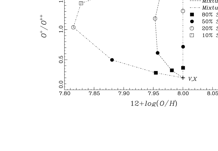
Figure 7: Diagnostic diagrams showing how the measured oxygen abundance, electron temperature, and ionization parameter (represented by $O^{+}/O^{++}$) changes as nebulae with different $T_{e}$ and $O^{+}/O^{++}$ are mixed in various proportions. Crosses mark the physical conditions of the basis spectra, S,T,U,V,W,X (see Table 3). Line styles distinguish gaseous mixtures of the standard spectrum, $S$, ($T_{e}(O^{++})=13,000$ K, $O^{+}/O^{++}=0.2$), with each of the other spectra. Symbols trace the decreasing contribution of the standard spectrum, $S$. The top panel shows that even small amounts of a high-temperature nebular component systematically bias derived electron temperatures (oxygen abundances) to higher (lower) values. For realistic temperature fluctuations and ionization variations, O/H is underestimated by 0.05 to 0.2 dex.

We begin by mixing the emission line spectrum of the standard sample, $S$, with the spectra of samples T,U,V,W,X in ratios of 80:20, 50:50, 20:80, and 10:90. Our standard nebular software is then used to analyze the resulting composite spectrum. Figure 7 displays the resulting electron temperatures, oxygen abundances, and $O^{+}/O^{++}$ ratios derived for the composite samples. Different symbols denote samples comprised of 80% (filled squares), 50% (filled circles), 20% (open circles), and 10% (open squares) of the standard sample, $S$. Crosses designate the physical conditions of the basis spectra, T,U,V,W,X, and S, used to construct the composite spectra. Line styles denote combinations of spectra T+S (dash-dot-dot line), U+S (solid line), V+S (dashed line), W+S (dotted line) and X+S (dash-dot line).

Figure 7 (top panel) shows that, as the spectrum S ($T_{e}(O^{++})$=13,000 K, $O^{+}/O^{++}=0.2$) is increasingly diluted with gas from spectrum U ($T_{e}$=11,000 K, $O^{+}/O^{++}=0.2$), the measured electron temperature decreases smoothly, while the measured oxygen abundance becomes slightly underestimated by up to 0.02 dex. For example, when the mixture of the composite spectrum is 80% S and 20% U (filled square on the solid line) the derived electron temperature is 12,750 K. The derived oxygen abundance is 12+log(O/H)=7.99, an underestimate by 0.01 dex. As the composite spectrum becomes 50% S and 50% U (solid line, filled circle) the derived oxygen abundance is underestimated by 0.02 dex. As the composite mixture becomes dominated by spectrum U (open circle and then open square) the derived physical conditions converge once again toward the temperature of basis spectrum U (11,000 K) and toward the initial oxygen abundance of both spectra, 12+log(O/H)=8.0.

When spectrum S is combined with spectrum V ($T_{e}$=11,000 K, $O^{+}/O^{++}=0.2$) the measured deviation from 12+log(O/H)=8.0 becomes more pronounced, up to 0.05 dex. The lower panel of Figure 7 shows a smooth progression in the measured $O^{+}/O^{++}$ ratio from 0.2 to 2.0. The mixture of spectrum S with spectrum W ($T_{e}$=9000 K, $O^{+}/O^{++}=0.2$) shows a substantial systematic deviation from constant metallicity. When the fraction of the lower temperature, lower ionization gas represented by spectrum W reaches 50% to 90% of the total emission line flux, the oxygen abundance is underestimated by 0.1 to 0.2 dex! A similar underestimate of the oxygen abundance results from spectrum X ($T_{e}$=9000 K, $O^{+}/O^{++}=2.0$). Figure 7 demonstrates that temperature fluctuations, modeled in the simplest possible way as a two-temperature medium, are the primary cause for over-estimation of the electron temperature and under-estimation of the oxygen abundance. Ionization parameter variations further exacerbate the systematic underestimate of oxygen abundances. Figure 7 shows that the addition of even a small quantity of high temperature gas (10%) creates a significant overestimate of the mean electron temperature.

Figure 7 demonstrates that the measured electron temperature, $T_{e}(O^{++})$, is sensitive to the physical conditions in the hottest $O^{++}$ zone of an H II region due to the strongly non-linear dependence of [O III] $\lambda$4363 on $T_{e}$. Furthermore, the electron temperature, $T_{e}(O^{++})$, in the $O^{++}$ zone is usually different than the electron temperature in lower-ionization $O^{+}$, $N^{+}$, $S^{+}$ zones at larger radii. Since $T_{e}(O^{+})$ or $T_{e}([S~{}II])$ is seldom measured directly, most nebular analyses procedures, including ours, adopt an empirical estimate based on the measured $T_{e}(O^{++})$ and photo-ionization modeling (Pagel et al. 1992; Skillman & Kennicutt 1993). However, in the presence of temperature fluctuations, or, in the limiting case of a two-temperature medium, the derived [O III] electron temperatures are weighted toward the high-temperature medium. Application of a naively–computed $T_{e}(O^{++})$ artificially decreases the total abundance by underestimating the oxygen abundance of both the $O^{++}$ zone and the $O^{+}$ zones.

A additional underestimate of the total metal abundance results if a large fraction of the nebular medium has a low ionization parameter. This is because estimates of $T_{e}(O^{+})$ derived from $T_{e}(O^{++})$ via an empirical relation based on photoionization models (Equation 1) will be inappropriately high. They systematically overestimate $T_{e}(O^{+})$, and underestimate the oxygen contribution from the dominant $O^{+}$ zones. While photoionization models can simulate the expected ionization structure of an ideal Stromgren sphere under a variety of ionization conditions, they do not take into account emission from the extended ionized (predominantly low-U) filaments and shells that are seen in actual galaxies. Since important factors such as the porosity of H II regions, the ionizing source of the extended shells and filaments, and the origin of the variation in DIG content from galaxy to galaxy are still uncertain, it is unlikely that these structures will soon be incorporated into photoionization models.

3 The Case of Spiral Galaxies

Like their low-mass counterparts, star-forming spiral galaxies also exhibit a range of ionization and temperature conditions throughout their ISM. However, except those with strong optical bars, they also show considerable radial chemical gradients, often exceeding an order of magnitude (Searle 1971; Villa-Costas & Edmunds 1992; Zaritsky, Kennicutt & Huchra 1994; Martin & Roy 1994). Global spectra of spiral galaxies will necessarily encompass a wide range of metallicities. In this section we consider whether it is possible to use global galaxy spectra, even in the presence of true chemical variations, to measure a “mean” or “indicative” systemic metallicity.

In high-metallicity H II regions ($12+{\log}(O/H)\geq 8.5$), the temperature sensitive [O III] $\lambda$4363 line is very weak, and it is seldom detected. Nevertheless, the oxygen abundance can be estimated using only the [O II] $\lambda$3727, [O III] $\lambda\lambda$4959,5007, and H$\beta$ lines using the method proposed by Pagel et al. (1979) and subsequently developed by many authors. For high-metallicity ($12+{\log}(O/H)\geq 8.5$) H II regions, there exists a monotonic relationship between the ratio of observed collisionally-excited emission line intensities,

$$R_{23}\equiv(I_{3727}+I_{4959}+I_{5007})/H\beta,$$ (5)

and the oxygen abundance of the nebula. In practice, only one of the [O III] lines is required, since $I_{5007}\simeq 2.87I_{4959}$ for all temperatures and densities encountered in H II regions. In the most metal-rich H II regions, $R_{23}$ is a minimum because the high metal abundance produces efficient cooling, reducing the electron temperature and the level of collisional excitation. $R_{23}$ increases in progressively more metal-poor nebula since lower metal abundance means reduced cooling, elevated electron temperatures, and a higher degree of collisional excitation. However, the relation between $R_{23}$ and O/H becomes double valued below about 12+log(O/H)=8.4 ($Z=0.3Z_{\odot}$). Figure 8 illustrates this double-valued behavior. In Figure 8, we plot a variety of published calibrations between $R_{23}$ and O/H, including McGaugh (1991: solid line), Zaritsky, Kennicutt, & Huchra, (1994: dashed line), McCall, Rybski, & Shields (1985: dotted line), Edmunds & Pagel (1984: dash-dot line), and Dopita & Evans (1986: dash-dot-dot line). On the upper, metal-rich branch of the relationship, the various calibrations show a dispersion of 0.2 dex at a fixed value of $R_{23}$. This dispersion represents the inherent uncertainties in the calibration which are based on photoionization modeling and observed H II regions (see original works for details). For metal abundances progressively lower than 12+log(O/H)$\simeq$8.2, $R_{23}$ decreases once again. On this lower branch, although the reduced metal abundance further inhibits cooling and raises the electron temperatures, the intensities of the [O II] and [O III] lines drop because of the greatly reduced abundance of oxygen in the ISM. On the lower, metal-poor branch of the relationship, a second parameter, the ionization parameter $U$, becomes important, in additional to $R_{23}$. This can be seen in the offset between the three solid lines from the calibration of McGaugh (1991). A varying ionization parameter may lead to a similar value of $R_{23}$ for different oxygen abundances. In Figure 8 we represent the approximate ionization parameter in terms of the easily observable line ratio [O III]/[O II]. The solid lines show the oxygen abundance as a function of $R_{23}$ for [O III]/[O II] = 10, 1.0, and 0.1 which correspond (very roughly) to ionization parameters, $U$, of $10^{-1}$, $10^{-2}$, and $10^{-4}$.

Figure 8 serves as a useful diagnostic diagram for finding the oxygen abundances of nebulae when the electron temperature is not measured directly. The typical uncertainties using this empirical oxygen abundance calibration are $\pm 0.15$ dex, but are larger, ($\pm$0.25 dex) in the turn-around region near 12+log(O/H)$\sim$8.4 when ${\log}(R_{23})>0.7$. The most significant uncertainty involves deciding whether an observed object lies on the upper, metal-rich branch of the curve, or on the lower, metal-poor branch of the curve. For instance, a measurement of $\log(R_{23})=0.0$ could indicate either an oxygen abundance of 12+log(O/H)$\simeq$7.2 or 12+log(O/H)$\simeq$9.1. Knowledge of either the luminosity of the galaxy or the [N II] $\lambda$6584 intensity can help break the degeneracy. Because star-forming galaxies of all types in the local universe follow a luminosity-metallicity correlation (e.g., Lequeux et al. 1979; Talent 1980; Skillman, Kennicutt, & Hodge 1989, ZKH), objects more luminous than $M_{B}\simeq-18$ have metallicities larger than 12+log(O/H)$\simeq$8.3, placing them on the upper branch of the curve. However, it has not yet been established whether galaxies at earlier epochs conform to the same relationship as local galaxies. An even better discriminator is the ratio [O III]$\lambda$5007/[N II] $\lambda$6584 which is usually greater than $\sim$100 for galaxies with 12+log(O/H)$>$8.3 on the metal-rich branch (Edmunds & Pagel 1984). This is because objects which are considerably enriched in oxygen are generally more nitrogen-rich as well, while the most metal-poor galaxies on the lower branch of the $R_{23}$ relation have very weak [N II] lines. Figure A1(b) of Edmunds & Pagel (1984) shows the monotonic sequence of the ratio [O III] $\lambda$5007/[N II] $\lambda 6584$ as a function of metallicity. If the [N II] $\lambda 6584$ line can be measured, we believe it will provide the most useful way to break the $R_{23}$ degeneracy in the absence of a measured electron temperature.

3.1 Individual H II Regions and Global Spiral Spectra

The compilation of H II region spectra in spiral galaxies presented by Zaritsky, Kennicutt, & Huchra (1994; ZKH) provides an excellent dataset to explore the utility of global metallicity measurements in galaxies with chemical gradients. We compiled a subset of spectra for 194 HII regions in 22 galaxies from ZKH and Kennicutt & Garnett (1996). We use our own remeasurements of the emission line ratios in the subsequent analysis.

We estimate the integrated [O II]/H$\beta$ and [O III]/H$\beta$ emission line ratios for each galaxy in the following way. Spectra of the individual HII regions from ZKH are used to define the range of [O II]/H$\beta$ and [O III]/H$\beta$ as a function of galactocentric radius. For NGC 5457 (M101) we use data from Kennicutt & Garnett (1996). In order to provide a meaningful estimate, we restrict the analysis to galaxies with at least 8 measured HII regions, spanning most of the radial range over which significant star formation takes place, and for which data on the radial distribution of H$\alpha$ emission are available. The actual number of HII regions measured ranges from 8 in NGC 4725 and NGC 5033 to 42 in M 101. Typical values lie in the range 10–20. We subdivide each disk into 5–13 equal-sized radial zones, with the number of zones depending on the number and distribution of HII regions; the mean line ratios in each zone are derived from the averages of the individual nebular line ratios. In a few instances a zone did not contain a measured HII region, and in such cases the local line ratios were interpolated from the two adjacent zones.

In order to derive disk-integrated line ratios, we compute a weighted radial average with the spectrum at each radius weighted by the relative H$\alpha$ surface brightness at each radius and the area contained in each zone. The H$\alpha$ radial profiles are derived from H$\alpha$ CCD images from Martin & Kennicutt (1998) and unpublished imaging from the original ZKH program, using an ellipse-fitting surface photometry routine. We sum [O II]/H$\beta$ and [O III]/H$\beta$ ratios for each galaxy to derive an integrated $R_{23}$ index for each galaxy, as given in Equation 5. In the calculations presented here we use the reddening-corrected HII region line strengths, convolved with the observed (uncorrected) H-alpha emission distributions, because this most faithfully duplicates the actual weighting when the integrated spectrum of a galaxy is observed. Table 4 lists the integrated line strengths and $R_{23}$ values for each galaxy, along with the number of HII regions used to derive these average values.

In Figure 9 we plot the integrated [O II] (log [O II]/H$\beta$) versus [O III] (log [O III]/H$\beta$) line strengths for each galaxy determined in this way (large triangles), as well as the [OII] and [O III] strengths for the individual HII regions in the same galaxy sample (dots). This comparison shows that the most of the integrated spectra lie along the same excitation/abundance sequence that is defined by the individual HII region. Such a correspondence would not necessarily be predicted a priori, because the HII region abundance sequence is not entirely linear, and one might expect the average spectra to be systematically displaced from the sequence. The tendency for the integrated spectra to lie on the excitation sequence partly reflects the limited range of abundance and excitation in many disks (especially barred systems), and the radial concentration of star formation in others.

It is clear from Figure 9 that the integrated [O II] and [O III] line strengths mimic those of individual HII regions, but how do the corresponding “mean” abundances compare to the actual abundances in the disks? In order to address this question we apply the $R_{23}$ calibration of ZKH to the integrated $R_{23}$ values in Table 4, to estimate a mean abundance for each galaxy. The ZKH calibration is only valid for HII regions which lie on the metal-rich branch of the R23 relation (see discussion above in Section 3), but this condition is satisfied for the sample considered here, with the exception of the outermost HII regions in M101, where $T_{e}$-based abundances were used.

Figure 10 illustrates how well the weighted-average mean nebular spectrum characterizes the overall galaxy abundance. In Figure 10 we compare the empirical abundances derived from the integrated spectra with the actual disk abundances from ZKH, measured at 0.4 times the corrected isophotal radius (25.0 mag arcsec^-2 in $B$). The latter abundances are listed in Table 4, along with two other characteristic abundances from ZKH, that measured at a fixed linear radius of 3 kpc (using distances given in ZKH), and the abundance at 0.8 exponential scale lengths (also given in ZKH). Figure 10 shows that the integrated [O II] and [O III] emission-line strengths provide an excellent estimate of the mean abundance of the disk, corresponding roughly to the value at 40% of the optical radius of the disk (indicated for reference by the solid line in Figure 10). The dispersion about the mean relation is very small, $\pm$0.05 dex. On the basis of these results we conclude that the beam-smearing effects from sampling large numbers of HII regions in the disk have a small effect on characterizing the mean abundance of galaxies, even those with substantial abundance gradients, relative to the intrinsic uncertainties in the R23 method itself.

Although these results offer assurances that the effects of averaging the composite spectra of large numbers of discrete HII regions do not seriously hamper the measurement of a mean disk abundance, there are other systematic effects, not incorporated into our simulations, that may affect the derived abundances more significantly. One such effect is dust reddening, which will tend to depress the flux of [O II] $\lambda$3727 relative to [O III] and H$\beta$ and tend to cause the mean abundance to be overestimated (for galaxies on the upper branch of the $R_{23}$–O/H relation). In our simulations we used the measured (i.e., reddened) line strengths when simulating the integrated spectra, so this effect is already incorporated into the comparisons shown in these Figures. To test the effects of reddening on the integrated spectra we carried out an identical comparison using reddening-corrected spectra, and the resulting O/H abundances change only slightly, increasing by 0.06 dex on average. A potentially more serious effect may be the contribution to the integrated spectrum of diffuse ionized gas, as discussed in Section 2.3. This gas tends to be characterized by stronger [O II] emission and weaker [OIII] emission than discrete HII regions of the same abundance (e.g., Hunter 1994, Martin 1997). However the same data show that the sum of [O II] and [O III] line strengths ($R_{23}$) does not change substantially, so including the diffuse gas may preserve the information on mean abundances, at least in the metallicity range probed here. However it would be useful to test this conclusion directly using actual integrated spectra of spiral galaxies. Finally, the effects of stellar absorption of H$\beta$ in integrated spectra of spirals can be very significant (see Section 4.2) and must be corrected for in the measurements of the integrated spectrum (Kennicutt 1992). Overall, the practicalities of measuring integrated emission-line strengths in spiral galaxies probably pose a much more challenging problem than the actual interpretation of the composite nebular spectrum.

4 The Effect of Underlying Stellar Absorption and Low Signal-to-Noise Spectra

In the previous two sections we show that global galaxy spectra can provide reliable information on the chemical properties of distant galaxies which exhibit high equivalent width emission lines. However, except for the most vigorously star-forming objects, the integrated spectra of most large galaxies are dominated by stellar continuum, rather than nebular emission. In some galaxies with strong post-starburst stellar populations, the nebular Balmer line emission is erased by stellar atmospheric absorption. Only 7 of the 24 global spectra of normal spiral and elliptical galaxies obtained by Kennicutt (1992) show measurable [O II], [O III], and H$\beta$ emission lines needed for empirical oxygen abundance determinations. However, a larger fraction of irregular and peculiar spiral galaxies show the requisite emission lines. In this section, we discuss the effects of low signal-to-noise spectra and stellar absorption which limit the precision of nebular abundance measurements from global spectra.

4.1 Uncertainties due to Low Signal-to-Noise

Because the empirical calibration between $R_{23}$ and oxygen abundance has an intrinsic uncertainty of 0.2 dex (40%), the total error budget will be dominated by this uncertainty even when the observed emission line spectra have low signal-to-noise. For example, a spectrum with a signal-to-noise of 8:1 (12%) on each of the [O II], [O III], and H$\beta$ emission lines will yield an uncertainty of 25% on $R_{23}$ or $\delta({\log}R_{23})\simeq$0.1 This observational uncertainty propagates into an O/H uncertainty of 0.1–0.2 dex, depending on the local slope of the calibration curve in Figure 8. This quantity is smaller than, or comparable to the uncertainty of the calibration curve, $\sim$0.2 dex, based on photoionization modeling. Thus, to within the accuracy of the strong-line calibration, even modest signal-to-noise spectra can yield useful indications of a galaxy’s gas-phase oxygen abundance.

4.2 Uncertainties due to Stellar Balmer Line Absorption

In high signal-to-noise nebular spectra, the observed ratios of H$\alpha$/H$\beta$, H$\gamma$/H$\beta$, and H$\delta$/H$\beta$, compared to theoretical values, simultaneously constrain the amount of reddening from intervening dust, and the degree to which the stellar atmospheric absorption lines reduce the measured nebular Balmer emission. In practice, global galaxy spectra, especially at high redshift, will seldom have the signal-to-noise and wavelength coverage necessary to decouple these effects. In the absence of high-quality Balmer line measurements, we recommend that a statistical correction be applied to the measured strength of the Balmer emission lines, principally H$\beta$. For integrated galaxy spectra presented here, and for the global spectra presented in Kennicutt (1992) the amount of underlying stellar absorption, Abs(H$\beta$), runs from 1Å to 6 Å, with a mean of 3 Å. (see also McCall, Rybski, & Shields 1985; Izotov, Thuan, & Lipovetsky 1994 for a sample of observations). We recommend that a statistical correction of $+3\pm 2$ Å be applied to H$\beta$ measurements from global galaxy spectra. When the signal-to-noise ratio of H$\beta$ is low, the uncertainty of $\pm$2 Å will act as an additional error term. For example, for spectra where H$\beta$ has an equivalent width of 8, the statistically important $+3\pm 2$ Å correction on EW(H$\beta$) introduces an additional 25% uncertainty on the strength of H$\beta$. This uncertainty must be accounted for in the total error budget.

4.3 Uncertainty due to Un-measured Ionization Species

An empirical measurement of the oxygen abundance using the method outlined in Section 3 requires measurements of the emission line strengths for both of the dominant species of oxygen, [O III] $\lambda\lambda$4959,5007, [O II] $\lambda$3727, and H$\beta$. However, complications due to limited wavelength coverage, or contamination from night sky lines and atmospheric absorption bands may preclude measurement of the necessary emission lines for objects at unfavorable redshifts. Fortunately, measurement of either [O III] $\lambda$4959 or [O III] $\lambda$4959, along with [O II] $\lambda$3727 and H$\beta$, is sufficient to measure oxygen abundances. The fixed theoretical ratio of $\lambda$5007/$\lambda$4959 is $\sim$2.9 for all electron temperatures and densities encountered in photoionized H II regions (although ratios as higher than 3 are sometimes measured in H II regions, and are more commonly seen in supernova remnants). Thus, the strength of one line can be computed from the other, and the accuracy of the O/H determination is not diminished.

Oxygen abundances become highly uncertain in the case where [O II] $\lambda$3727 is not measured. [O II] $\lambda$3727 is a crucial diagnostic for indicating the ionization parameter, fraction of diffuse ionized gas, and possible contamination from AGN-like excitation mechanisms. $O^{+}$ may be the dominant ionization state in low-ionization H II regions. The global spectra in Kennicutt (1992) indicate that $O^{+}$ is the dominant ionization species in more than half of the 24 galaxies with suitable emission lines. Ratios of $O^{+}/O^{++}$ range from 0.10 to 4.0. Neglecting the contribution from $O^{+}$ may result in errors as small as 10% in the case of high-ionization nebulae, up to a factor of 4 in galaxies dominated by low-ionization gas. However, the metallicity-excitation sequence observed in Figure 9 between [O III]/H$\beta$ and [O II]/H$\beta$ suggests that, for the majority of normal galaxies on the metal-rich branch of the $R_{23}$ relation, a measurement of [O III]/H$\beta$ can constrain the value of [O II]/H$\beta$ to within a factor of 3. The converse is not true. An observed ratio [O II]/H$\beta$ does not correspond to a any well-constrained [O III]/H$\beta$ ratio since the scatter in [O III]/H$\beta$ at a given [O II]/H$\beta$ exceeds a factor of 10. Attempts to estimate oxygen abundances without an [O II]/H$\beta$ ratio must carry very large uncertainties of 0.5 dex, while attempts to measure oxygen abundances without an [O III]/H$\beta$ ratio have uncertainties exceeding 1 dex.

5 Prospects for Measuring the Metallicities of High-Redshift Emission Line Galaxies

We have shown that global galaxy spectra which are dominated by normal H II regions can provide reliable information on the gas-phase chemical abundances, even in objects with variable gas temperature and chemical properties. In summary, chemical analysis using nebular optical emission lines falls into three regimes.

1). [O III] $\lambda$4363 is detected along with [O II] $\lambda$3727, [O III] $\lambda\lambda$4959,5007 and H$\beta$: In the best case scenario, the [O III] $\lambda$4363 line can be used to derive an electron temperature for the emitting gas, and chemical abundance ratios can be estimated using standard nebular analysis techniques (e.g., Osterbrock 1989). In local galaxies, [O III] $\lambda$4363 is generally detected only in galaxies with 12+log(O/H)$\leq$8.4 ($Z\leq 0.3~{}Z_{\odot}$). Based on spatially-resolved and global spectra of local irregular galaxies which are chemically homogeneous but contain varying temperature and ionization conditions, we find that the [O III] $\lambda$4363 line strength provides a firm upper limit on the mean electron temperature of the ionized gas. The oxygen abundance derived using this $T_{e}$ is therefore a firm lower limit. Our empirical results in local galaxies, combined with modeling realistic mixtures of H II regions with varying physical conditions, suggests that a statistical correction factor of $\Delta(O/H)=+0.1$ or $\Delta{T_{e}}=-1000$ K be applied to physical parameters derived from global galaxy spectra.

2) [O III] $\lambda$4363 is not detected but [O II] $\lambda$3727, [O III] $\lambda\lambda$4959,5007 and H$\beta$ are measured: Most of the time, the temperature sensitive [O III] $\lambda$4363 will not be detected due to either limited signal-to-noise or intrinsically weak lines in metal-rich nebulae. In this case, the empirical strong-line calibration in Figure 8 can still be used to derive an oxygen abundance to within $\pm$0.2 dex (the uncertainty in the model calibrations) if the [O III] $\lambda\lambda$5007,4959, [O II] $\lambda$3727, and H$\beta$ lines are measured with a signal-to-noise of at least 8:1. A major difficulty with this method is that the relation between oxygen abundance and $R_{23}$ is double valued, requiring some assumption or rough $a~{}priori$ knowledge of a galaxy’s metallicity in order to locate it on the appropriate branch of the curve. We suggest that the [N II]/[O III] line ratios may be useful in breaking this degeneracy, if they can be measured.

Analytic fits to the curves in Figure 8 may assist in computing the oxygen abundances from measured line ratios. Zaritsky, Kennicutt, & Huchra (1994) provide a polynomial fit to their average of three previous calibrations shown in Figure 8. This mean relation is good for the upper, metal-rich regime only:

$$12+log(O/H)=9.265-0.33x-0.202x^{2}-0.207x^{3}-0.333x^{4}\ (ZKH~{}1994)$$ (6)

where

$$x\equiv\ \log{R_{23}}\equiv\ \log\Biggr{(}{{[O~{}II]\lambda 3727+[O~{}III]\lambda\lambda 4959,5007}\over{H\beta}}\Biggr{)}$$ (7)

McGaugh (1991) computed a more extensive calibration based on a set of photoionization models which take into account the effects of varying ionization parameter in both the metal-rich and metal-poor regimes as shown in Figure 8. McGaugh (1998) provides analytic expressions for the metal-poor (lower) branch,

$$12+log(O/H)_{l}=12-4.944+0.767x+0.602x^{2}-y(0.29+0.332x-0.331x^{2}),$$ (8)

and for the metal-rich (upper) branch,

$$12+log(O/H)_{u}=12-2.939-0.2x-0.237x^{2}-0.305x^{3}-0.0283x^{4}-$$ (9)

$$y(0.0047-0.0221x-0.102x^{2}-0.0817x^{3}-0.00717x^{4}),$$ (10)

where

$$y\equiv\ \log(O_{32})\equiv\ \log\Biggr{(}{{[O~{}III]\lambda\lambda 4959,5007}\over{[O~{}II]\lambda 3727}}\Biggr{)}$$ (11)

These analytic expressions to the semi-empirical calibration of McGaugh (1991, 1998) fit the models to within an RMS of $\leq$0.05 dex.

3) Only [O III] $\lambda\lambda$4959,5007 and H$\beta$ are measured: Very crude oxygen abundances may be derived from the ratio of [O III] $\lambda\lambda$4959,5007/H$\beta$ even if the [O III] $\lambda$4363 and [O II] $\lambda$3727 are not measured. This requires both an assumption about the objects location on the bi-valued $R_{23}$ relation, and an assumption about the ionization parameter which leads to an estimate of the [O II] $\lambda 3727$ line strength. Uncertainties in this case must exceed 0.5 dex.

4) The spectrum has a signal-to-noise less than 8:1, or one of the necessary emission lines are not measured: In this worst-case scenario, the uncertainties on the O/H ratio will exceed a factor of 3 (0.5 dex). Conclusions about the chemical nature of the object under consideration will be speculative at best.

Given that star-forming regions appear to be plentiful at higher redshifts, the prospects appear good for measuring chemical abundances in distant galaxies, even with coarse spatial resolution of ground-based telescopes. The coming generation of near-infrared spectrographs on large telescopes will make it possible to trace the chemical evolution of the universe using emission line regions in a manner complementary to absorption-line techniques.

Figure 1: Global spectra for each galaxy observed in this work, not corrected for reddening or redshift. Flux units are relative units only, since the data were acquired using drift scan techniques. Each spectrum is plotted a second time, scaled by a factor of 40 for display purposes.

Figure 2: The electron temperature, $T_{e}$, derived from the [O III] $\lambda$4363 measurements versus the signal-to-noise ratio of the [O III] $\lambda$4363 line for multiple measurements in six nearby irregular galaxies. Small symbols represent measurements of individual H II regions or localized measurements, while large symbols with error bars designate the results from global spectra. For most objects, [O III] $\lambda$4363 in the global spectrum has a S/N ratio that lies in the middle of the S/N distribution of small apertures. The electron temperature measured from the global spectra consistently fall near the highest electron temperatures measured from localized spectra. This is consistent with global nebular galaxy spectra being biased toward regions of highest temperature and surface brightness.

Figure 3: The oxygen abundance, $12+{\log}(O/H)$, derived from the [O III] $\lambda$4363 measurements versus the signal-to-noise ratio of the [O III] $\lambda$4363 line for multiple measurements in six nearby irregular galaxies. Small symbols represent measurements of individual H II regions or localized measurements, while large symbols with error bars designate the results from global spectra. For most objects, [O III] $\lambda$4363 in the global spectrum has a S/N ratio that lies in the middle of the S/N distribution of small apertures. The but the oxygen abundances measured from the global spectra consistently fall among the lowest values measured from localized spectra. This is consistent with global nebular galaxy spectra being biased toward regions of highest temperature and surface brightness.

Figure 4: Absolute blue magnitude versus oxygen abundance, $12+{\log}(O/H)$, for six nearby irregular galaxies. Small symbols represent measurements of individual H II regions or localized measurements, while large symbols with error bars designate the results from global spectra. This figure demonstrates that the oxygen abundances measured from the global spectra consistently fall among the lowest values measured from localized spectra. This is consistent with global nebular galaxy spectra being biased toward regions of highest temperature and surface brightness. The data plotted here also show the well-known correlation between luminosity and oxygen abundance for irregular galaxies (cf. Skillman 1989)

Figure 5: The [O III] electron temperatures and the resulting oxygen abundances for 69 positions in 6 metal-poor galaxies. Small symbols represent measurements of individual H II regions or localized measurements, while large symbols denote global measurements. The solid line illustrates the direction along which O/H measurements would scatter due to random uncertainties in the adopted electron temperature. Variations of 0.1–0.2 dex in O/H within galaxies are consistent with variations in the adopted electron temperature of 1000 K — 2000 K. The global measurement for each galaxy consistently exhibits the largest $T_{e}$ and the smallest oxygen abundance.

Figure 6: The ratio of singly to doubly ionized oxygen, $O^{+}/O^{++}$, versus the difference between oxygen abundance derived from global spectra and the mean of the spatially-resolved individual measurements. As seen in Figure 4, global spectra consistently yield O/H measurements 0.05 — 0.2 dex below the mean of the localized measurements within the same galaxy. There is a weak correlation, consistent with the possibility that the global spectra in galaxies dominated by doubly-ionized oxygen (i.e., those with $O^{+}/O^{++}<0.5$) show a larger deviation from the mean measurement within that galaxy compared to galaxies where $O^{+}$ and $O^{++}$ contribute more equally. In none of the galaxies does $O^{+}$ dominate the nebular emission. The magnitude of the offset suggests a systematic error of $\sim 0.1$ dex when using global spectra to derive oxygen abundances from measured electron temperatures and line strengths.

Figure 8: The calibration of oxygen abundance, 12+log(O/H), as a function of the strong line ratio ${\log}(R_{23})\equiv\log([I_{3727}+I_{4959}+I_{5007}]/H\beta$) from several different authors. Strong line ratios can reliably indicate the oxygen abundance to within the accuracy of the model calibrations, $\pm 0.15$ dex. However, the relationship is double-valued, requiring some $a~{}priori$ knowledge of a galaxy’s metallicity in order to determine its correct location on the upper or lower branch of the curve. At low metallicities, a given value of $R_{23}$ may yield different oxygen abundances depending on the ionization parameter of the gas. We show the effect of varying the ionization parameter using the models of McGaugh (1991) in terms of the observable line ratio, $(I_{4959}+I_{5007})/I_{3727}$. The uncertainties using this empirical calibration are $\pm 0.15$ dex, but larger, $\pm$0.25 dex n the turn-around region near 12+log(O/H)$\sim$8.4.)

Figure 9: log([O III]/H$\beta$) versus log([O II]/H$\beta$) for H II regions in 22 spiral galaxies from ZKH and the literature. Triangles denote the global emission line spectrum for each galaxy constructed from the sum of its constituent H II region spectra (small symbols). The global spectra follow the same excitation/ metallicity sequence as individual H II regions. Labels at each end of the sequence denote approximate metallicities of 2 $Z_{\odot}$ and 0.3 $Z_{\odot}$.

Figure 10: The characteristic O/H ratio at a fiducial radius of 0.4 isophotal radii as tabulated by ZKH versus the O/H ratio derived from the global nebular spectrum for each galaxy. The global spectra produce oxygen abundances which are in excellent agreement (0.1 dex) with the value at 0.4 isophotal radii (25.0 mag arcsec^-2 in $B$).

References

- (1) Aller, L. H. 1942, ApJ, 95, 52
- (2) Aller, L. H. 1990, PASP, 102, 1097
- (3) Brodie, J. P., & Huchra, J. P. 1991, ApJ, 379, 157
- (4) Dopita, M. A., & Evans, I. N. 1986, ApJ, 307, 431
- (5) Edmunds, M. G. & Pagel, B. E. J. 1984, MNRAS, 211, 507
- (6) Faber, S. M. 1973, ApJ, 179, 423
- (7) Ferguson, A. M., Wyse, R. G., Gallagher, J. S. III, & Hunter, D. A. 1996, AJ, 111, 2265
- (8) French, H. B., 1980, ApJ, 240, 41
- (9) Garnett, D. R. 1990, ApJ, 363, 142
- (10) Gonzalez-Delgado, R. M., Pŕez, Enrique, Tenorio-Tagle, G., et al. 1994, ApJ, 437, 239
- (11) Heckman, T. M. 1980, A&A, 87, 152
- (12) Hummer, D. G., & Storey, P. J. 1987, MNRAS, 224, 801
- (13) Hunter, D. A. 1994, AJ, 107, 565
- (14) Hunter, D. A. & Gallagher, J. S. III 1990, ApJ, 362, 480
- (15) Hunter, D. A., & Gallagher, J. S. III. 1997, 475, 65
- (16) Izotov, Y., Thuan, T. T., & Lipovetsky, V. A. 1994, ApJ, 435, 647
- (17) Kennicutt, R. C. Jr. 1992, ApJS, 79, 255 (K92)
- (18) Kennicutt, R. C. Jr., & Garnett, D. R. 1996, ApJ, 456, 504
- (19) Kingdon, J. B., & Ferland, G. J. 1995, ApJ, 691
- (20) Kobulnicky, H. A. in Abundance Profiles: Diagnostic Tools for Galaxy History, ASP Conf. Ser. Vol. 147, eds. D. Friedli, M. Edmunds, C. Robert, & L. Drissen (San Francisco: ASP)
- (21) Kobulnicky, H. A., & Skillman, E. D. 1996, ApJ, 471, 211
- (22) Kobulnicky, H. A., & Skillman, E. D. 1997, ApJ, 489, 636
- (23) Kobulnicky, H. A. & Zaritsky, D. 1998, ApJ, in press
- (24) Lauroesch, J. T., Truran, J. W., Welty, D. E., & York, D. G. 1996, PASP, 108, 641
- (25) Lequeux, J., Peimbert, M., Rayo, J. F., Serrano, A., & Torres–Peimbert, S. 1979, A&A, 80, 155
- (26) Lilly, S. J., Le Févre, O., Hammer, F., & Crampton, D. 1996, ApJ, 460, L1
- (27) Liu, X., & Danziger, J. 1995, MNRAS, 263, 256
- (28) Madau, P. Ferguson, H. C., Dickinson, M. E., Giavalisco, M., Steidel, C. C., & Fruchter, A. 1996, MNRAS, 283, 1388
- (29) Martin, C. L. 1996, ApJ, 465, 680
- (30) Martin, C. L. 1997, ApJ, 491, 561
- (31) Martin, C. L., & Kennicutt, R. C. 1998, ApJ, in press
- (32) Martin, P., & Roy, J. R. 1994, 424, 599
- (33) McCall, M. L., Rybski, P. M., & Shields, G. A. 1985, ApJS, 57, 1 (MRS)
- (34) McGaugh, S. 1991, ApJ, 380, 140
- (35) McGaugh, S. 1998, private communication
- (36) Oke, J. B. 1990, AJ, 99, 1621
- (37) Olofsson, K. 1995, A&AS, 111, 570
- (38) Osterbrock, D. E. 1989, Astrophysics of Gaseous Nebulae and Active Galactic Nuclei, University Science Books:Mill Valley CA, p. 134
- (39) Pagel, B. E. J. 1986, PASP, 98, 1009
- (40) Pagel, B. E. J., Edmunds, M. G., Blackwell, D. E., Chun, M. S., & Smith, G. 1979, MNRAS, 189, 95
- (41) Pagel, B. E. J., Simonson, E. A., Terlevich, R. J., & Edmunds, M. G. 1992, MNRAS, 255, 325
- (42) Peimbert, M. 1967, ApJ, 150, 825
- (43) Peimbert, M. 1975, ARA&A, 13, 113
- (44) Peimbert, M. 1996, in The Analysis of Emission Lines, Poster Papers from the Space Telescope Science Institute Symposium in Honor of the 70th Birthdays of D. E. Osterbrock and M. J. Seaton, ed. R. E. Williams & M. Livio, (Baltimore: STScI), 165
- (45) Pérez, E. 1997, MNRAS, 290, 465
- (46) Richer, M. G., & McCall, M. L. 1995, ApJ, 445, 642
- (47) Searle, L. 1971, ApJ, 168, 327
- (48) Shields, G. A. 1990, ARA&A, 28, 525
- (49) Skillman, E. D., Bomans, D. J., & Kobulnicky, H. A. 1996, ApJ, 474, 205
- (50) Skillman, E. D., & Kennicutt, R. C. 1993, ApJ, 411, 655
- (51) Skillman, E. D., Kennicutt, R. C., & Hodge, P. 1989, ApJ, 347, 875 (SKH)
- (52) Stasińska, G. 1990, A&AS, 83, 501
- (53) Steidel, C. C., Giavalisco, M., Pettini, M., Dickinson, M., Adelberger, K. L. 1996, ApJ, 462, 17
- (54) Steigman, G., Viegas, S. M., & Gruenwald, R. 1997, ApJ, 490, 187.
- (55) Talent, D. L. 1980, Ph.D. Thesis, Rice University
- (56) Veilleux, S., & Osterbrock, D. E. 1987, ApJS, 63, 295
- (57) Villa-Costas, M. B., & Edmunds, M. G. 1992, MNRAS, 259, 121
- (58) Walsh, J. R., & Roy, J-R. 1989, MNRAS, 239, 297
- (59) Walsh, J. R., & Roy, J-R. 1993, MNRAS, 262, 27
- (60) Walter, D. K., Dufour, R. J., & Hester, J. J. 1992, ApJ, 397, 196
- (61) Zaritsky, D., Kennicutt, R. C., & Huchra, J. P. 1994, ApJ, 420, 87 (ZKH)