The Visual Orbit of $\iota$ Pegasi

Abstract

We have determined the visual orbit for the spectroscopic binary $\iota$ Pegasi with interferometric visibility data obtained by the Palomar Testbed Interferometer in 1997. $\iota$ Pegasi is a double-lined binary system whose minimum masses and spectral typing suggests the possibility of eclipses. Our orbital and component diameter determinations do not favor the eclipse hypothesis: the limb-to-limb separation of the two components is 0.151 $\pm$ 0.069 mas at conjunction. Our conclusion that the $\iota$ Peg system does not eclipse is supported by high-precision photometric observations.

The physical parameters implied by our visual orbit and the spectroscopic orbit of Fekel and Tomkin (1983) are in good agreement with those inferred by other means. In particular, the orbital parallax of the system is determined to be 86.9 $\pm$ 1.0 mas, and masses of the two components are determined to be 1.326 $\pm$ 0.016 M_☉ and 0.819 $\pm$ 0.009 M_☉ respectively.

1 Introduction

$\iota$ Pegasi (HR 8430, HD 210027) is a nearby, short-period (10.2 d) binary system with a F5V primary and a $\sim$ G8V secondary in a circular orbit. $\iota$ Peg was first discovered as a single-lined spectroscopic binary by Campbell (1899), and the first spectroscopic orbital elements were estimated by Curtis (1904). Several other single-line studies were made, notably Petrie and Phibbs (1949) and Abt and Levy (1976). In the context of a lithium abundance study, Herbig (1965) noted that lines from the $\iota$ Peg secondary were visible at red wavelengths. Lithium abundances for both the primary (Herbig (1965); Conti & Danzinger (1966); Duncan (1981); Lyubimkov et al. (1991)) and the secondary (Fekel & Tomkin (1983); Lyubimkov et al. (1991)) indicate the system is very young ($\sim$ 8 $\times$ 10⁷ yr, Fekel & Tomkin (1983), 1.7 $\pm$ 0.8 $\times$ 10⁸ yr, Lyubimkov et al. (1991)) and both components are close to the zero-age main sequence. Both components of $\iota$ Peg are also believed to have solar-type abundances (Lyubimkov et al. (1991)).

Following Herbig’s implicit suggestion, Fekel and Tomkin (1983, hereafter FT) made radial velocity measurements of both $\iota$ Peg components at 643 nm, and computed a definitive spectroscopic orbit and inferred a probable G8V spectral classification for the secondary. FT’s orbit was noteworthy as it indicated that the minimum masses for the two components were very near the model values for the spectral types, suggesting a “reasonable prospect” for eclipses in the system (FT). Subsequent photometric monitoring by automated photometry projects in Arizona, at Palomar Observatory, and in Pasadena failed to show any evidence for eclipses (see §5). FT also questioned synchronous rotation of the secondary. However, Gray (1984), from somewhat higher resolution spectroscopic data, argued that both components are in synchronous rotation.

Herein we report a determination of the $\iota$ Peg visual orbit from near-infrared, long-baseline interferometric visibility measurements taken with the Palomar Testbed Interferometer. PTI is a 110-m K-band (2 - 2.4 $\mu$m) interferometer located at Palomar Observatory, and described in detail elsewhere (Colavita et al. (1994); Colavita et al. 1999a ). The minimum PTI fringe spacing is roughly 4 mas at the sky position of $\iota$ Peg, allowing us to resolve this binary system. The procedures we have used to determine $\iota$ Peg’s visual orbit are similar to other visual orbits determined for spectroscopic binaries using the Mark III Interferometer at Mt. Wilson (Pan et al. (1990); Armstrong et al. 1992a ; Armstrong et al. 1992b ; Pan et al. (1992); Hummel (1993); Pan et al. (1993); Hummel et al. (1994, 1995)), and the NPOI Interferometer at Anderson Mesa, AZ (Hummel et al. (1998)). The analogy between $\iota$ Peg and the short-period, small angular scale binaries studied in Hummel et al. (1995) and Hummel et al. (1998) is especially apt.

2 Observations

Pan attempted to determine a visual orbit for $\iota$ Peg using the Mark III interferometer at Mt. Wilson, but the significant brightness difference in the two components at 800 nm made the observations difficult (Pan (1997)). The apparent contrast ratio in the $\iota$ Peg system decreases in the K-band, allowing a reliable orbit determination with PTI observations.

The observable used for these observations is the fringe contrast or visibility (squared) of an observed brightness distribution on the sky. Normalized in the interval [0,1], a single star exhibits visibility modulus given in a uniform disk model by:

$$V=\frac{2\;J_{1}(\pi B\theta/\lambda)}{\pi B\theta/\lambda}$$ (1)

where $J_{1}$ is the first-order Bessel function, $B$ is the projected baseline vector magnitude at the star position, $\theta$ is the apparent angular diameter of the star, and $\lambda$ is the center-band wavelength of the interferometric observation. (We consider corrections to the uniform disk model from limb darkening in §4.) The expected squared visibility in a narrow pass-band for a binary star such as $\iota$ Peg is given by:

$$V^{2}_{nb}(\lambda)=\frac{V_{1}^{2}+V_{2}^{2}\;r^{2}+2\;V_{1}\;V_{2}\;r\;\cos(\frac{2\pi}{\lambda}\;{\bf{B}}\cdot{\bf{s}})}{(1+r)^{2}}$$ (2)

where $V_{1}$ and $V_{2}$ are the visibility moduli for the two stars alone as given by Eq. 1, $r$ is the apparent brightness ratio between the primary and companion, ${\bf{B}}$ is the projected baseline vector at the system sky position, and ${\bf{s}}$ is the primary-secondary angular separation vector on the plane of the sky (Pan et al. (1990); Hummel et al. (1995)). The $V^{2}$ observables used in our $\iota$ Peg study are both narrow-band $V^{2}$ from seven individual spectral channels (Colavita et al. 1999a ), and a synthetic wide-band $V^{2}$, given by an incoherent SNR-weighted average $V^{2}$ of the narrow-band channels in the PTI spectrometer (Colavita 1999b ). In this model the expected wide-band $V^{2}$ observable is approximately given by an average of the narrow-band formula over the finite pass-band of the spectrometer:

$$V^{2}_{wb}=\frac{1}{n}\sum_{i}^{n}V^{2}_{nb-i}(\lambda_{i})$$ (3)

where the sum runs over the n = 7 channels with wavelengths $\lambda_{i}$ covering the K-band (2 - 2.4 $\mu$m) of the PTI spectrometer in its 1997 configuration. Separate calibrations and hypothesis fits to the narrow-band and synthetic wide-band $V^{2}$ datasets yield statistically consistent results, with the synthetic wide-band data exhibiting superior fit performance. Consequently we will present only the results from the synthetic wide-band data.

$\iota$ Peg was observed by PTI on 24 nights between 2 July and 8 Sept 1997. In each night $\iota$ Peg was observed in conjunction with calibration objects multiple times during the night. Each observation (“scan”) was from 120 – 130 seconds in duration. For each scan we computed a mean $V^{2}$ value through methods described in Colavita (1999b). We assumed the measured rms in the internal scatter to be the error in $V^{2}$. For the purposes of this analysis we have restricted our attention to four calibration objects, two primary calibrators within 5^∘ of $\iota$ Peg (HD 211006 and HD 211432), and two ancillary calibrators within 15^∘ of $\iota$ Peg (HD 215510 and HD 217014 – 51 Pegasi). The suitability of 51 Peg (a known radial velocity variable) as a calibrator at PTI is addressed in Boden et al. (1998b). Table 1 summarizes the relevant parameters on the calibration objects used in this study. In particular we have estimated our calibrator diameters based on a model diameter on 51 Peg of 0.72 $\pm$ 0.06 mas implied by a linear diameter of 1.2 $\pm$ 0.1 R_☉ (adopted by Marcy et al. (1997)) and a parallax of 65.1 $\pm$ 0.76 mas from Hipparcos (ESA (1997); Perryman et al. (1997)).

The calibration of $\iota$ Peg $V^{2}$ data is performed by estimating the interferometer system visibility ($V^{2}_{sys}$) using calibration sources with model angular diameters, and then normalizing the raw $\iota$ Peg visibility by $V^{2}_{sys}$ to estimate the $V^{2}$ measured by an ideal interferometer at that epoch (Mozurkewich et al. (1991); Boden et al. 1998a ). We calibrated the $\iota$ Peg $V^{2}$ data in two different ways: (1) with respect to the two primary calibration objects, resulting in our primary dataset containing 112 calibrated observations over 17 nights, and (2) an unbiased average of the primary and ancillary calibrators, resulting in our secondary dataset containing 151 observations over 24 nights. The motivation for constructing these two datasets, which are clearly not independent, is that the determination of the orbital solution and component diameters is sensitive to calibration uncertainties. Comparison of the solutions derived from the two datasets allow us to quantitatively assess this uncertainty.

Object	Spectral	Star	Sky Separation	Diam. WRT
Name	Type	Magnitude	From $\iota$ Peg	Model 51 Peg
HD 211006	K2III	5.9 V/3.4 K	3.6∘	1.06 $\pm$ 0.05
HD 211432	G9III	6.4 V/3.7 K	3.2∘	0.70 $\pm$ 0.05
HD 215510	G6III	6.3 V/3.9 K	11∘	0.85 $\pm$ 0.06
HD 217014	G2.5V	5.9 V/4.0 K	12∘	(0.72 $\pm$ 0.06)

Table 1: 1997 PTI $\iota$ Peg Calibration Objects Considered in our Analysis. The relevant parameters for our four calibration objects are summarized. The apparent diameter values are determined by a fit to our $V^{2}$ data calibrated with respect to a model diameter for HD 217014 (51 Peg) of 0.72 $\pm$ 0.06 mas (Marcy et al. (1997); ESA (1997)).

3 Orbit Determination

The estimation of the $\iota$ Peg visual orbit is made by fitting a Keplerian orbit model with visibilities predicted by Eqs. 2 and 3 directly to the calibrated (narrow-band and synthetic wide-band) $V^{2}$ data on $\iota$ Peg (see Armstrong et al. 1992b ; Hummel (1993); Hummel et al. (1995)). The fit is non-linear in the Keplerian orbital elements, and is therefore performed by non-linear least-squares methods (i.e. the Marquardt-Levenberg method, Press et al. (1992)). As such, this fitting procedure takes an initial estimate of the orbital elements and other parameters (e.g. component angular diameters, brightness ratio), and refines the model into a new parameter set which best fits the data. However, the chi-squared surface has many local minima in addition to the global minimum corresponding to the true orbit. Because Marquardt-Levenberg strictly follows a downhill path in the $\chi^{2}$ manifold, it is necessary to thoroughly survey the space of possible binary parameters to distinguish between local minima and the true global minimum. In the case of $\iota$ Peg the parameter space is significantly narrowed by the high-quality spectroscopic orbit and inclination constraint near 90^∘ (FT). Furthermore, the Hipparcos distance determination sets the rough scale of the semi-major axis (ESA (1997)).

In addition, as the $V^{2}$ observable for the binary (Eqs. 2 and 3) is invariant under a rotation of 180^∘, we cannot differentiate between an apparent primary/secondary relative orientation and its mirror image on the sky. In order to follow the FT convention for T₀ at primary radial velocity maximum, in our analysis of $\iota$ Peg we have defined T₀ to be at a component separation extremum, yielding an extremum in component radial velocities for the circular orbit. We have additionally required our fit T₀ to be within half a period of the projected FT determination to differentiate between primary radial velocity maximum and minimum. Even with our determination of T₀ so defined there remains a 180^∘ ambiguity in our determination of the longitude of the ascending node, $\Omega$.

We used a preliminary orbital solution computed by Pan (1996) by separation vector techniques (see Pan et al. (1990) for a discussion of the method), and refined it into the best-fit orbit shown here. We further conducted an exhaustive search of the binary parameter space that resulted in the same best-fit orbit, which is in fact the global minimum in the $\chi^{2}$ manifold.

Figure 1 depicts the apparent relative orbit of the $\iota$ Peg system. Most striking is the observation that the circular orbit of the system (see below) is very nearly eclipsing. From our primary dataset we find a best fit orbital inclination of 95.67 $\pm$ 0.21 degrees. With model angular diameters of 1.0 and 0.7 mas for the primary and secondary components respectively (§4), and an apparent semi-major axis of 10.33 $\pm$ 0.10 mas, this inclination is about 0.87^∘ from apparent limb-to-limb contact. This is consistent with the lack of photometric evidence for eclipses despite several photometry campaigns on the $\iota$ Peg system (§5).

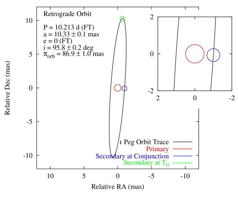
Figure 1: Visual Orbit of $\iota$ Pegasi. The relative visual orbit of $\iota$ Peg is depicted, with the primary and secondary rendered at T₀ (maximum primary radial velocity) and apparent conjunction. The inset shows a closeup of the system at apparent conjunction. By our model the $\iota$ Peg orbit is nearly, but not quite eclipsing, being approximately 0.87^∘ in inclination from apparent grazing eclipses.

Table 3 lists the complete set of $V^{2}$ measurements in the primary dataset and the prediction based on the best-fit orbit model for $\iota$ Peg. Figure 2 shows two graphical comparisons between our $V^{2}$ data on $\iota$ Peg and the best-fit model predictions. Figure 2a gives four consecutive nights of PTI $V^{2}$ data from our primary dataset on $\iota$ Peg (18 – 21 July 1997), and $V^{2}$ predictions based on the best-fit model for the system. Figure 2b gives an additional seven consecutive nights (12 – 18 August 1997) with the same quantities plotted. These are the two longest consecutive-night sequences in our data set. The model predictions are seen to be in excellent absolute and statistical agreement with the observed data, with a primary dataset average absolute $V^{2}$ deviation of 0.014, and a $\chi^{2}$ per Degree of Freedom (DOF) of 0.75.

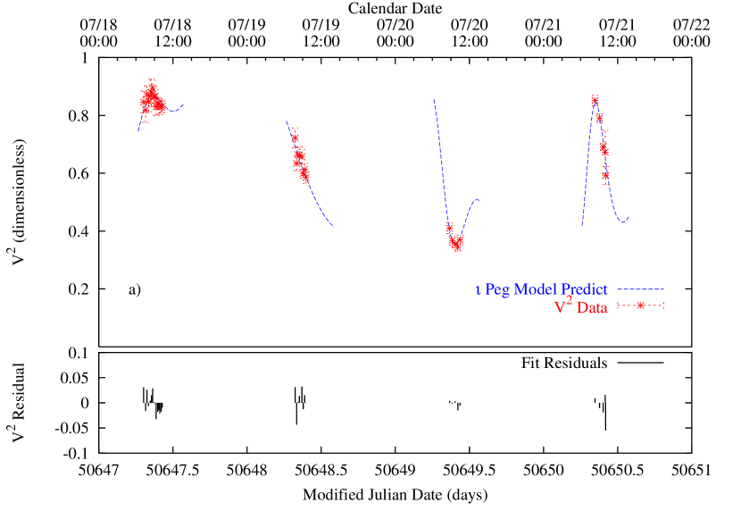
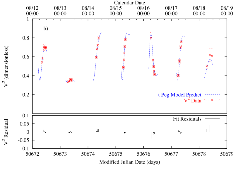
Figure 2: $V^{2}$ Fit of $\iota$ Pegasi. a) Four consecutive nights (18 – 21 July 1997) of calibrated $V^{2}$ data on $\iota$ Peg, and $V^{2}$ predictions from the best-fit model for the system. In the lower frame we give $V^{2}$ residuals between the calibrated data and best-fit model. b) An additional seven consecutive nights (12 – 18 August 1997) of data on $\iota$ Peg, with model predicts and fit residuals. The model is in good agreement with the calibrated data, with a $\chi^{2}$/DOF of 0.75 and an average absolute $V^{2}$ residual of 0.014.

Figure 3 gives two examples of the $\chi^{2}$ fit projected into orbital parameter subspaces. Figure 3a shows a surface of $\chi^{2}$/DOF projected into the subspace of orbit semi-major axis and relative component brightness, with all other parameters held to their best-fit values. Inset is a closeup of a contour plot of the $\chi^{2}$/DOF surface indicating location of the best-fit parameter values, and contours at +1, +2, and +3 of $\chi^{2}$/DOF significance. Figure 3b gives the $\chi^{2}$/DOF surface in the subspace of orbital inclination and longitude of the ascending node. Again, the inset gives best-fit parameter values, and contours at +1, +2, and +3 of $\chi^{2}$/DOF significance. All indications are that the best-fit model for the $\iota$ Peg system is in excellent agreement with our $V^{2}$ data, and that data uniquely constrain the parameters of the visual orbit.

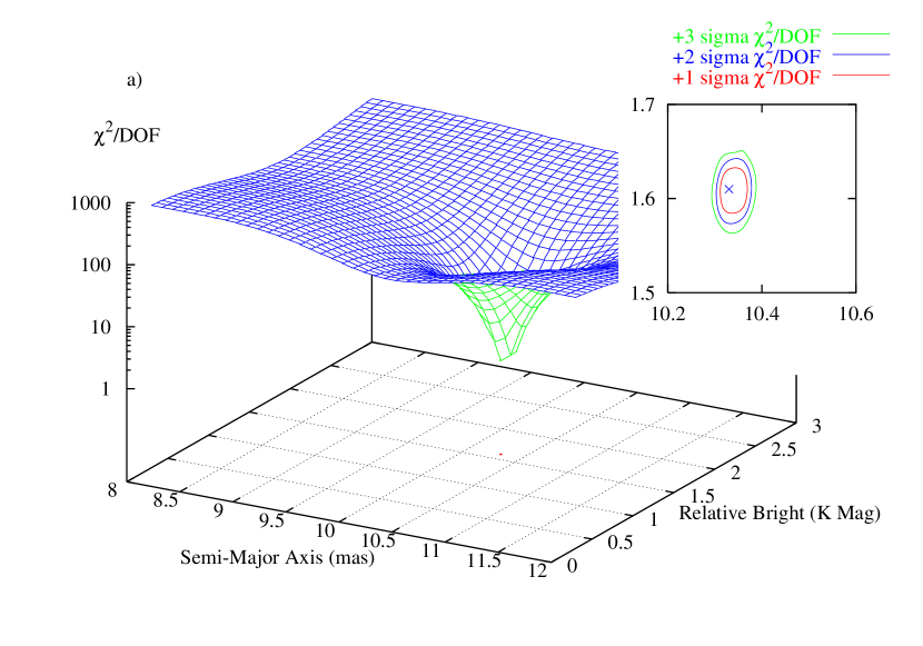
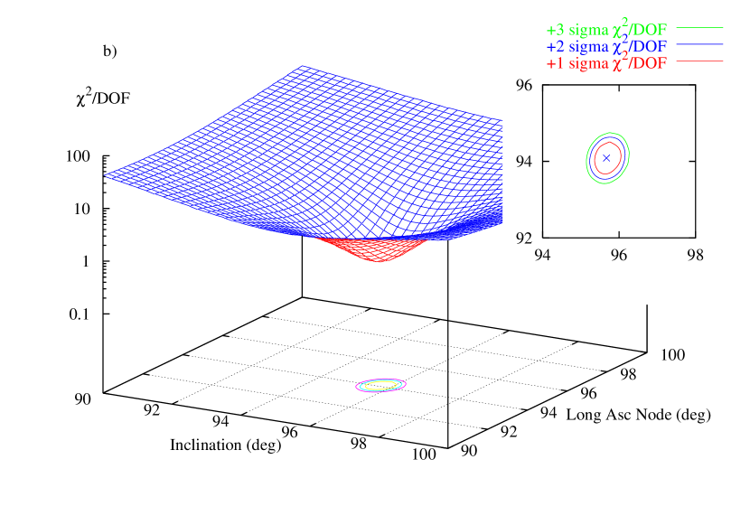
Figure 3: $\chi^{2}$/DOF Fit Surfaces for $\iota$ Pegasi Primary Dataset. a) $\chi^{2}$/DOF surface in the subspace of orbit semi-major axis and relative component brightness. Inset is a closeup of a contour plot surface indicating location of the best-fit parameter values, and contours at +1, +2, and +3 of $\chi^{2}$/DOF significance. b) $\chi^{2}$/DOF surface in the subspace of orbital inclination and longitude of the ascending node, with inset giving surface contour closeup.

Spectroscopic (from FT) and visual orbital parameters of the $\iota$ Peg system are summarized in Table 3. We present the results for our primary and secondary datasets separately. For the parameters we have estimated from our interferometric data we quote a total one-sigma error in the parameter estimates, and the one-sigma errors in the parameter estimates from statistical (measurement uncertainty) and systematic error sources. In our analysis the dominant forms of systematic error are: (1) uncertainties in the calibrator angular diameters (Table 1); (2) the uncertainty in our center-band operating wavelength ($\lambda_{0}\approx$ 2.2 $\mu$m), which we have taken to be 20 nm ($\sim$1%); (3) the geometrical uncertainty in our interferometric baseline ( $<$ 0.01%); and (4) uncertainties in orbital parameters we have constrained in our fitting procedure (e.g. period, eccentricity). Different parameters are affected differently by these error sources; our estimated uncertainty in the $\iota$ Peg orbital inclination is dominated by measurement uncertainty, while the uncertainty in the angular semi-major axis is dominated by uncertainty in the wavelength scale. Conversely, we have assumed that all the uncertainty quoted by FT in the $\iota$ Peg spectroscopic parameters is statistical. Finally, we have listed the level of statistical agreement in the visual orbit parameters in our two solutions (the absolute residual between the two estimates divided by the RSS of their statistical errors). The two solutions are in good statistical agreement, giving us confidence we have properly characterized our calibration uncertainties.

Particularly remarkable is the agreement between T₀ (quoted as the epoch of maximum primary radial velocity for the $\iota$ Peg circular orbit) and period as determined by FT, and T₀ as determined in our primary dataset, separated from the FT determination by 523 cycles. FT quote an $\iota$ Peg period accurate to roughly 1 part in 10⁶, resulting in a propagated uncertainty in T₀ at the epoch of our observations of 7 $\times$ 10^-3 days. This FT-extrapolated T₀ differs from our 1997 T₀ determination by 8 $\times$ 10^-4 days, an agreement of roughly 0.1 sigma. A similar comparison with the secondary dataset solution is less spectacular, an agreement at 0.7 sigma. Clearly the extraordinary quoted accuracy of the $\iota$ Peg period determination by FT (made by combining their 1977 – 1982 data with spectroscopy from the mid-30s – Petrie & Phibbs (1949)) seems well justified compared to our visual orbit. Consequently we have assumed the FT value for the $\iota$ Peg period.

Following FT we have assumed a circular orbit for the system. Fitting our primary dataset for an eccentricity in the system yields an estimate of 1.5 $\times$ 10^-3 $\pm$ 1.3 $\times$ 10^-3. The assumption of a circular orbit seems well justified.

Orbital	FT	PTI 1997
Parameter	1983	Primary Dataset	Secondary Dataset	Stat Agr
Period (d)	10.213033	10.213033	10.213033
	$\pm$ 1.3 $\times$ 10-5	(assumed)	(assumed)
T0 (HJD)	2445320.1423	2450661.5578	2450661.5634	1.26
		$\pm$ 3.6 (3.3/1.5) $\times$ 10-3	$\pm$ 3.3 (3.0/1.5) $\times$ 10-3
$e$	0 (assumed)	0 (assumed)	0 (assumed)
KA (km s-1)	48.1 $\pm$ 0.2
KB (km s-1)	77.9 $\pm$ 0.3
$i$ (deg)		95.67 $\pm$ 0.22 (0.22/0.03)	96.03 $\pm$ 0.20 (0.20/0.03)	1.21
$\Omega$ (deg)		94.09 $\pm$ 0.23 (0.22/0.05)	94.03 $\pm$ 0.25 (0.24/0.05)	0.03
$a$ (mas)		10.33 $\pm$ 0.10 (0.02/0.10)	10.32 $\pm$ 0.11 (0.02/0.11)	0.35
$\Delta$ K (mag)		1.610 $\pm$ 0.021	1.610 $\pm$ 0.021	0.23
		(0.007/0.020)	(0.007/0.020)
$\chi^{2}$/DOF		0.75	1.0
$\overline{|R_{V^{2}}|}$		0.014	0.016
Nscans		112	151

Table 3: Orbital Parameters for $\iota$ Peg. Summarized here are the apparent orbital parameters for the $\iota$ Peg system as determined by FT, and our PTI primary and secondary datasets. For parameters estimated from our PTI observations we separately quote one sigma errors from both statistical and systematic sources (listed as $\sigma_{stat}$/$\sigma_{sys}$), and the total error as the sum of the two in quadrature. We have also included the level of statistical agreement between visual orbit parameters from our two solutions; the parameters estimated separately from the primary and secondary datasets are in good agreement in relation to the statistical component of their error estimates. We have quoted the longitude of the ascending node parameter ($\Omega$) as the angle between local East and the orbital line of nodes (and the relative position of the secondary at T₀), measured positive in the direction of local North. Due to the degeneracy in our $V^{2}$ observable there is a 180^∘ ambiguity in $\Omega$. Finally, the fit $\chi^{2}$/DOF and mean absolute $V^{2}$ residual ($\overline{|R_{V^{2}}|}$) is listed for both solutions.

4 Physical Parameters

Physical parameters derived from the $\iota$ Peg primary dataset visual orbit and the FT spectroscopic orbit are summarized in Table 4. We use the primary dataset solution because it is the most free from possible sky position-dependent systematic effects (as the secondary dataset includes the ancillary calibrators), but we note the two orbital solutions yield statistically consistent results. Notable among the physical parameters for the system is the high-precision determination of the component masses for the system, a virtue of the precision of the FT radial velocities on both components and the high inclination of the orbit. We estimate the masses of the F5V primary and putative G8V secondary components as 1.326 $\pm$ 0.016 M_☉ and 0.819 $\pm$ 0.009 M_☉ respectively. Our mass values agree well with mass estimates of 1.33 $\pm$ 0.08 M_☉ and 0.9 $\pm$ 0.2 M_☉ respectively made by Lyubimkov et al. (1991) based on evolutionary models and spectroscopic measurements of component effective temperatures and surface gravities.

The Hipparcos catalog lists the parallax of $\iota$ Peg as 85.06 $\pm$ 0.71 mas (ESA (1997)). The distance determination to $\iota$ Peg based on the FT radial velocities and our apparent semi-major axis and inclination is 11.51 $\pm$ 0.13 pc, corresponding to an orbital parallax of 86.91 $\pm$ 1.0 mas, consistent with the Hipparcos result at roughly 2% and 1.5 sigma.

FT list main-sequence model linear diameters for the two $\iota$ Peg components as 1.3 and 0.9 R_☉ respectively (FT). At a distance of approximately 11.5 pc this corresponds to apparent angular diameters of 1.0 and 0.7 mas for the primary and secondary components respectively. We have fit for the uniform-disk angular diameter for both components as a part of the orbit estimation, and find best fit apparent diameters of 0.98 $\pm$ 0.05 and 0.70 $\pm$ 0.10 mas. Because we have limited spatial frequency coverage in our data, following Mozurkewich et al. (1991) and Quirrenbach et al. (1996) we have estimated the limb-darkened diameters of the components from a correction to the uniform-disk diameter based on the solar limb-darkening at 2 $\mu$m given by Allen (1982). The limb-darkened diameters for the primary and secondary components are 1.0 $\pm$ 0.05 and 0.71 $\pm$ 0.10 mas respectively. For both the primary and secondary components our fits for apparent diameter are in good agreement with main-sequence model diameters.

The observed K-magnitude of the $\iota$ Peg system (2.623 $\pm$ 0.016 – Carrasco et al. (1991), 2.656 $\pm$ 0.002 – Bouchet et al. (1991)) and our estimates of the distance and relative K-photometry (Table 3) of the system allows the determination of the absolute magnitude of both components separately. Using the Bouchet et al. (1991) K-photometry we obtain M_K values of 2.574 $\pm$ 0.025 and 4.182 $\pm$ 0.030 for the primary and secondary components respectively. Both of these M_K values are consistent (within quoted scatter) to the empirical mass-luminosity relation for nearby low-mass, main-sequence stars given by Henry & McCarthy (1992, 1993). In particular, our M_K value for the primary is 0.010 mag brighter than the mass-luminosity prediction (Henry & McCarthy (1992)), while the 4.18 M_K value for the secondary is roughly 0.28 magnitudes dimmer than the prediction (Henry & McCarthy (1993)). Both values are well within the quoted scatter of the mass-luminosity models. A second check on the absolute K-magnitude estimates can be extracted from the model calculations of Bertelli et al. (1994), who predict absolute K-magnitudes of 2.616 $\pm$ 0.048 and 4.254 $\pm$ 0.039 for our estimated primary and secondary masses respectively for main-sequence stars with solar-type abundances at an age of 1.7 $\pm$ 0.8 $\times$ 10⁸ yr (Lyubimkov et al. (1991)).

Physical	Primary	Secondary
Parameter	Component	Component
a (10-2 AU)	4.54 $\pm$ 0.03 (0.03/0.0002)	7.35 $\pm$ 0.03 (0.03/0.0003)
Mass (M☉)	1.326 $\pm$ 0.016 (0.016/0.0001)	0.819 $\pm$ 0.009 (0.009/0.0001)
Sp Type (FT)	F5V	G8V
Model Diameter (mas)	1.0	0.7
UD Fit Diameter (mas)	0.98 $\pm$ 0.05 (0.01/0.05)	0.70 $\pm$ 0.10 (0.03/0.10)
LD Fit Diameter (mas)	1.0 $\pm$ 0.05 (0.01/0.05)	0.71 $\pm$ 0.10 (0.03/0.10)
System Distance (pc)	11.51 $\pm$ 0.13 (0.05/0.12)
$\pi_{orb}$ (mas)	86.91 $\pm$ 1.0 (0.34/0.94)
MK (mag)	2.574 $\pm$ 0.025 (0.010/0.024)	4.182 $\pm$ 0.030 (0.019/0.028)

Table 4: Physical Parameters for $\iota$ Peg. Summarized here are the physical parameters for the $\iota$ Peg system as derived from the orbital parameters in Table 3. As for our PTI-derived orbital parameters we have quoted both total error and separate contributions from statistical and systematic sources (given as $\sigma_{stat}$/$\sigma_{sys}$).

5 Eclipse Search

A critical test of our visual orbit model is a high-precision photometric search for eclipses in $\iota$ Peg. Combined with our visual orbit (Table 3), our measured diameters (Table 4) imply an apparent limb-to-limb separation at conjunction of 0.151 $\pm$ 0.069 mas (using our limb-darkened diameter estimates). Our visual orbit and fit diameters do not favor the FT conjecture of possible eclipses in the $\iota$ Peg system. Conversely, were the inclination of the orbit near 90^∘, there would be significant primary eclipses with a duration of a few hours (6.8 hr for $i$ = 90^∘ – FT), and as large as 0.6 mag in V-band.

Several individuals have searched for signs of eclipses in the $\iota$ Peg system. In 1997 both Van Buren with the 60” telescope at Palomar (1997) and one of us (C.D.K.) at the Robinson Rooftop Observatory at Caltech in Pasadena (Koresko (1997)) searched for eclipses during primary and secondary eclipse opportunities respectively. Both searches resulted in non-detections at about the 0.1 mag levels.

More comprehensive and sensitive than the Southern California searches has been the program conducted by the Automated Astronomy Group at Tennessee State University. $\iota$ Peg was observed photometrically in 1984 with the Phoenix-10 automatic photoelectric telescope (APT) in Phoenix, AZ, and again in 1997-98 with the Vanderbilt/Tennessee State 16-inch APT at Fairborn Observatory near Washington Camp, AZ, in order to search for possible eclipses suggested by FT. Both telescopes observed $\iota$ Peg once per night through a Johnson V filter with respect to the comparison star HR 8441 (HD 210210, F1 IV) in the sequence C,V,C,V,C,V,C, where C is the comparison star and V is $\iota$ Peg. Three differential magnitudes (in the sense V-C) were computed from each nightly sequence, corrected for differential extinction, and transformed to the Johnson system. The three differential magnitudes from each sequence were then averaged together and treated as single observations thereafter. Because of the lack of accurate standardization in the Phoenix-10 data set, a -0.027 mag correction was added to each observation to bring those data in line with the 16-inch observations. The observations are summarized in Table 5. Column 4 gives the standard deviation of a single nightly observation from the mean of the entire data set and represents a measure of the precision of the observations. Further details on the telescopes, data acquisition, reductions, and quality control can be found in Young et al. (1991) and Henry (1995a,b).

APT	JD Range	# Obs.	Std. Dev.
	(+2400000)		(mag)
10-inch	45703 – 46065	78	0.0109
16-inch	50718 – 50829	66	0.0032

Table 5: Summary of APT Photometry on $\iota$ Peg.

The photometric observations summarized in Table 5 are plotted in Figure 4 against orbital phase of the binary computed from the FT-defined T₀ and period. For inclinations allowing eclipses of the two components, the phases of conjunction coinciding with primary and secondary eclipse opportunities are 0.25 and 0.75 respectively. FT estimated the total duration of a central eclipse ($i$ = 90^∘) to be roughly 6.8 hours or 0.027 phase units. Our photometric observations exclude this possibility and show no evidence for any partial eclipse to a precision of around 0.003 mag. The time of conjunction is uncertain by no more than a few minutes, and gaps in the data around the time of conjunction are no larger than about 0.005 phase units (1.2 hours). Thus, the possibility of all but the briefest of grazing eclipses are excluded by the APT photometry. In particular, using the two points nearest the primary conjunction opportunity (at -1.29 and +1.22 hours relative to the predicted conjunction respectively) constrain $|90-i|$ to be greater than 4.07^∘ and 4.10^∘ respectively at greater than 99% confidence, based on the model diameters and M_v estimates of 3.4 and 5.8 for the primary and secondary components respectively.

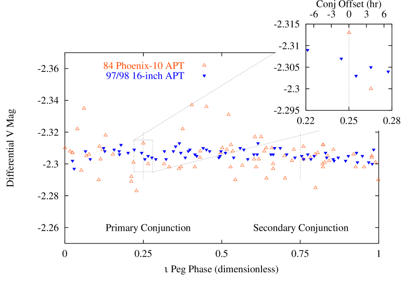
Figure 4: Photometric Observations of $\iota$ Peg. Differential photometric observations of $\iota$ Peg from the Phoenix-10 APT (open triangles) and the Vanderbilt/Tennessee State University 16-inch APT (filled triangles) plotted against orbital phase of the binary computed following FT. Phase 0.25 represents a time of conjunction with the secondary in front (primary eclipse opportunity). Inset we show a closeup of the data around the primary eclipse opportunity. (We have added a second horizontal scale relative to the eclipse opportunity in units of hours; a full eclipse in the $\iota$ Peg system would be roughly 7 hours in duration.) The photometric observations exclude the possibility of all but the briefest of grazing eclipses in the $\iota$ Peg system.

The components of most close binaries with orbital periods less than about one month rotate synchronously with the orbital period due to tidal action between the components (e.g. Fekel & Eitter (1989)). Such synchronous rotation is expected in $\iota$ Peg and is confirmed by the rotational broadening measurements of FT and Gray (1984) (c.f. Wolff & Simon (1997)). If the G8V secondary, which is much more convective than the F5V primary, is rotating synchronously, it would be expected to be photometrically variable on the orbital period at the level of a few percent due to starspot activity (Henry et al. (1999)). In fact, $\iota$ Peg is listed as a suspected variable star by Petit (1990), who reports variability at the 0.02 mag level in V. FT estimate that the secondary is roughly 2.7 mag fainter in the V band than the primary, so any apparent photometric variability of the secondary component will be diluted by a factor of about 12 by the primary component.

In order to search for this possible photometric variability in $\iota$ Peg, we performed a periodogram analysis of the 16-inch APT data. The analysis reveals a photometric period that is identical, within its uncertainty, to the spectroscopic period, a result that is consistent with the assumption of synchronous rotation. Likewise, the amplitude of 0.0037 mag, scaled by a factor of 12, results in a 4.4% variation, similar to the variability expected from rotational modulation of the spotted surface of the secondary diluted by the emission of the primary. Based on these results, we conclude that $\iota$ Peg is a low-amplitude variable star.

6 Summary

We have presented the visual orbit for the double-lined binary system $\iota$ Pegasi, and derived the physical parameters of the system by combining it with the earlier spectroscopic orbit of Fekel and Tomkin. The derived physical parameters of the two young stars in $\iota$ Peg are in reasonable agreement with the results of other studies of the system, and theoretical expectations for stars of these types. Noted by FT, the $\iota$ Peg system is nearly eclipsing; because our model visual orbit is so close to producing observable eclipses we have further presented high-precision photometric data which is consistent with our visual orbit model.

$\iota$ Peg represents a prototype of the binary system that PTI is well-suited to measure; the large magnitude difference between components in the visible is significantly mitigated in the near-infrared, making the accurate determination of the system parameters feasible.

References

- Allen (1982) Allen, C.W., Astrophysical Quantities, Athlone Press, 1982.
- (2) Armstrong, J.T. et al. 1992, AJ 104, 241.
- (3) Armstrong, J.T. et al. 1992, AJ 104, 2217.
- Bertelli et al. (1994) Bertelli, G., Bressan, A., Chiosi, C., Fagotto, F., and Nasi, E. 1994, A&AS 106, 275.
- (5) Boden, A.F. et al. 1998, Proc. SPIE 3350, 872.
- (6) Boden, A.F. et al. 1998, ApJ 504, L39.
- Bouchet et al. (1991) Bouchet, P., Manfroid, J., and Schmider, F.X. 1991, A&AS 91, 409.
- Campbell (1899) Campbell, W.W. 1899, ApJ 9, 310.
- Carrasco et al. (1991) Carrasco, L., Recillas-Cruz, E., Garcia-Barreto, A., Cruz-Gonzalez, I., and Serrano, A. 1991, PASP 103, 987.
- Colavita et al. (1994) Colavita, M.M. et al. 1994, Proc. SPIE 2200, 89.
- (11) Colavita, M.M. et al. 1999a, ApJ in press (astro-ph/9810262).
- (12) Colavita, M. 1999b, PASP in press (astro-ph/9810462).
- Conti & Danzinger (1966) Conti, P.S. and Danziger, I.J. 1966, ApJ 146, 383.
- Curtis (1904) Curtis, H.D. 1904, Lick Obs. Bull. 2, 172.
- Duncan (1981) Duncan, D.K. 1981, ApJ 248, 651.
- ESA (1997) ESA 1997, The Hipparcos and Tycho Catalogues, ESA SP-1200.
- Fekel & Tomkin (1983) Fekel, F. and Tomkin, J. 1983 (FT), PASP 95, 1000.
- Fekel & Eitter (1989) Fekel, F.C & Eitter, J.J. 1989, AJ 97, 1139.
- Gray (1984) Gray, D.F. 1984, PASP 96, 537.
- Henry & McCarthy (1992) Henry, T. and McCarthy, D. 1992, Proc. Comp. Double Star Research, IAU Col. 135, McAllister, H. and Hartikopf, W. ed.
- Henry & McCarthy (1993) Henry, T. and McCarthy, D. 1993, AJ 106, 773.
- (22) Henry, G.W. 1995a, in ASP Conf. Ser. 79, Robotic Telescopes: Current Capabilities, Present Developments, and Future Prospects for Automated Astronomy, ed. G.W. Henry & J.A. Eaton (San Francisco: ASP), 37.
- (23) Henry, G.W. 1995b, in ASP Conf. Ser. 79, Robotic Telescopes: Current Capabilities, Present Developments, and Future Prospects for Automated Astronomy, ed. G.W. Henry & J.A. Eaton (San Francisco: ASP), 44.
- Henry et al. (1999) Henry, G.W. et al. 1999, in preparation.
- Herbig (1965) Herbig, G.H. 1965, ApJ 141, 588.
- Hummel (1993) Hummel, C.A. et al. 1993, AJ 106, 2486.
- Hummel et al. (1994) Hummel, C. et al. 1994, AJ 107, 1859.
- Hummel et al. (1995) Hummel, C. et al. 1995, AJ 110, 376.
- Hummel et al. (1998) Hummel, C. et al. 1998, AJ in press.
- Koresko (1997) Koresko, C.D. 1997, http://gulliver.gps.caltech.edu/PTI/iota_Peg/iota_Peg_lightcurve.html
- Lyubimkov et al. (1991) Lyubimkov, L.S. , Polosukhina, N.S., and Rosgopchin, S.I. 1991, Astrofizika 34, 149.
- Marcy et al. (1997) Marcy, G.W. et al. 1997, ApJ 481, 926.
- Mozurkewich et al. (1991) Mozurkewich, D. et al. 1991, AJ 101, 2207.
- Pan et al. (1990) Pan, X. et al. 1990, ApJ 356, 641.
- Pan et al. (1992) Pan, X. et al. 1992, ApJ 384, 624.
- Pan et al. (1993) Pan, X., Shao, M., and Colavita, M. 1993, ApJ 413, L129.
- Pan et al. (1996) Pan, X. et al. 1996, BAAS 189, #32.03.
- Pan (1997) Pan, X. 1997, private communication.
- Perryman et al. (1997) Perryman, M.A.C. et al. 1997, A&A 323, L49.
- Petit (1990) Petit, M. 1990, A&AS 85, 971.
- Petrie & Phibbs (1949) Petrie, R.M., and Phibbs, E. 1949, Pub. Dominion Astrophys. Obs. 7, 205.
- Press et al. (1992) Press, W.H., Teukolsky, S.A., Vetterling, W.T., and Flannery, B.P. 1992, Numerical Recipes in C: The Art of Scientific Computing, Second Edition, Cambridge University Press.
- Quirrenbach et al. (1996) Quirrenbach, A. et al. 1996, A&A 312, 160.
- Van Buren (1997) Van Buren, D. 1997, private communication.
- Wolff & Simon (1997) Wolff, S.C. and Simon, T. 1997, PASP 109, 759.
- Young el al (1991) Young, A.T. et al. 1991, PASP 103, 221.