Confirmation of Eclipses in KPD 0422+5421, A Binary Containing a White Dwarf and a Subdwarf B Star

Abstract

We report additional photometric CCD observations of KPD 0422+5421, a binary with an orbital period of 2.16 hours which contains a subdwarf B star (sdB) and a white dwarf. There are two main results of this work. First, the light curve of KPD 0422+5421 contains two distinct periodic signals, the 2.16 hour ellipsoidal modulation discovered by Koen, Orosz, & Wade (1998) and an additional modulation at 7.8 hours. This 7.8 hour modulation is clearly not sinusoidal: the rise time is about 0.25 in phase, whereas the decay time is 0.75 in phase. Its amplitude is roughly half of the amplitude of the ellipsoidal modulation. Second, after the 7.8 hour modulation is removed, the light curve folded on the orbital period clearly shows the signature of the transit of the white dwarf across the face of the sdB star and the signature of the occultation of the white dwarf by the sdB star. We used the Wilson-Devinney code to model the light curve to obtain the inclination, the mass ratio, and the $\Omega$ potentials, and a Monte Carlo code to compute confidence limits on interesting system parameters. We find component masses of $M_{\rm sdB}=0.36^{+0.37}_{-0.16}\,M_{\odot}$ and $M_{\rm WD}=0.47^{+0.18}_{-0.16}\,M_{\odot}$ ($M_{\rm total}=0.86^{+0.52}_{-0.35}\,M_{\odot}$, 68 per cent confidence limits). If we impose an additional constraint and require the computed mass and radius of the white dwarf to be consistent with a theoretical mass-radius relation, we find $M_{\rm sdB}=0.511^{+0.047}_{-0.050}\,M_{\odot}$ and $M_{\rm WD}=0.526^{+0.033}_{-0.030}\,M_{\odot}$ (68 per cent confidence limits). In this case the total mass of the system is less than $1.4\,M_{\odot}$ at the 99.99 per cent confidence level. We briefly discuss possible interpretations of the 7.8 hour modulation and the importance of KPD 0422+5421 as a member of a rare class of evolved binaries.

1 Introduction

KPD 0422+5421 was first identified in the Kitt Peak Downes survey of blue stars at mid to low galactic latitudes (Downes 1986). It was classified as a hot, hydrogen-rich subdwarf B (sdB) star. The binary nature of this star was discovered by Koen, Orosz, & Wade (1998, hereafter KOW) who determined an orbital period of $P=0.0901795\pm(3\times 10^{-7})$ days (2.16 hours) using spectroscopic and photometric observations. KOW showed that the companion star of the sdB is a white dwarf, and determined masses of $M_{\rm sdB}=0.72\pm 0.26\,M_{\odot}$ and $M_{\rm WD}=0.62\pm 0.18\,M_{\odot}$ for the sdB star and white dwarf, respectively. KPD 0422+5421 has one of the shortest known orbital periods for a detached binary, and is one of only a few known binaries which contain an sdB star paired with a white dwarf. This binary has had an interesting past, given that it contains two evolved stars in a close orbit, and will have an interesting future, given the relatively short time-scale for merger due to the loss of orbital angular momentum via gravitational wave radiation ($\approx 1.5\times 10^{8}$ yr), which is comparable to the core He burning lifetime of an sdB star (Dorman, Rood, & O’Connell 1993).

The $U$ and $B$ light curves of KPD 0422+5421 presented in KOW are ellipsoidal, with amplitudes of $\approx 0.02$ mag. Ellipsoidal model fits to the light curves using the Wilson-Devinney (1971, hereafter W-D) code indicated a high inclination ($78^{\circ}$) which should produce an eclipsing geometry. The signature of the white dwarf transit across the face of the sdB star was predicted to be $\approx 0.006$ mag deep, lasting $\approx 27^{\circ}$ in phase ($\approx 10$ minutes of time). The presence of eclipses would be important since one could in principle then determine the geometry of the system reasonably well. However, the $U$ and $B$ light curves of KOW, which were obtained using high-speed photomultipliers, were sufficiently noisy that this subtle signature could not be clearly seen. We therefore obtained additional photometric observations using a CCD with the goal of obtaining a precise eclipse profile. We discuss below our observations, data reduction and analysis, and our results.

2 Observations and Data Reduction

We observed KPD 0422+5421 December 27-30, 1998 (all dates are UT) using the Kitt Peak 2.1 metre telescope and the T1KA $1024\times 1024$ CCD. The CCD was binned $2\times 2$ on chip, yielding a readout time of $\approx 11$ seconds and a scale of 0$\aas@@fstack{\prime\prime}$6 per pixel. Nearly all of the observations were made with a standard Kron $R$ filter (we used the KPNO “Harris set” $U\!BV\!R$$I$ filters). The exposure times ranged from 20 to 40 seconds. Care was taken to place the image of KPD 0422+5421 on the same region of the detector in order to minimize possible systematic errors introduced by flat-fielding errors. The observations on the first night were mostly taken through thin cirrus, while the other three nights were clear. The seeing was typically 1$\aas@@fstack{\prime\prime}$0 to 1$\aas@@fstack{\prime\prime}$2, although on some occasions the seeing was as low as 0$\aas@@fstack{\prime\prime}$75. We obtained a total of 2676 $R$-band images of KPD 0422+5421 covering 9.17 hours, 8.83 hours, 8.75 hours, and 9.83 hours on December 27 through December 30, respectively. On December 28 we also obtained images of a total of 38 standard stars in four different fields (RU 149, RU 152, PG 0918+029, PG 1047+003) from the list of Landolt (1992) in the $U$, $B$, $V$, $R$, and $I$ filters (airmass range 1.19 to 1.97), as well as three sets of images of KPD 0422+5421 in the same filters (airmasses of 1.44, 1.46, and 1.63).

Standard IRAF tasks were used to remove the electronic bias and to perform the flat-fielding corrections. The programs DAOPHOT IIe, ALLSTAR and DAOMASTER (Stetson 1987; Stetson, Davis, & Crabtree 1991; Stetson 1992a,b) were used to compute the photometric time series of KPD 0422+5421 and all of the field stars. The DAOPHOT and ALLSTAR codes were used because KPD 0422+5421 has a faint neighbour star $\approx 2\aas@@fstack{\prime\prime}3$ to the south ($\Delta R=5.1$) and because many of the bright field stars also have near neighbours. We used an iterative procedure to arrive at the final light curve. First, an automated DAOPHOT/ALLSTAR script was used to determine the positions and instrumental magnitudes of all the stars for each frame. Then using the stellar positions determined above, the DAOMASTER code was used to compute the mean pixel offsets for each image with respect to the first one. The pixel shifts were rounded to the nearest integer (to avoid interpolation in the shifting routine) and the images were then aligned so that they all had a common coordinate system. A deep “master” image was made by combining 101 images where the seeing was better than $\approx 0\aas@@fstack{\prime\prime}9$, and DAOPHOT and ALLSTAR were used to reduce this master image interactively. In the end we selected nineteen relatively bright and isolated field stars which gave the best fits to the empirical point spread function (PSF). The final “master photometry list” for this deep image had 838 stars, compared to the $\approx 300$ stars typically found by the daofind routine on any given single image. Next, the aligned images were reduced using another automated DAOPHOT/ALLSTAR script. In this case, the stars from the master photometry list were used in place of the initial stellar list generated by daofind for each image and the same 19 stars were used to fit the PSFs for each image. We found that the script using the larger master photometry list and common PSF stars gave much better results than the simple script used for the first iteration. Finally, the DAOMASTER code was used to robustly compute the mean magnitude offsets for each image and correct the magnitude system of each image to the magnitude system of the first image by adding a constant.

Figure 1: Top panels: the time series photometry of KPD 0422+5421 ($R$-band). In addition to the ellipsoidal modulation at 2.16 hours, a signal with a much longer period is evident. Bottom panels: the light curves of two nearby comparison stars, plotted using the same range in the $y$-axis as the top panels.

The observations of the Landolt standard stars were used to calibrate the DAOMASTER instrumental magnitudes to the standard system. We used the IRAF task phot to perform aperture photometry on the standard stars using a sequence of different sized apertures of radius 3 to 16 pixels (1$\aas@@fstack{\prime\prime}$8-9$\aas@@fstack{\prime\prime}$6). The IRAF implementation of the DAOGROW algorithm (Stetson 1990) was then used to fit the curve-of-growth function for each image and compute the optimal instrumental magnitudes for the $r=16$ pixel aperture. The resulting list of instrumental magnitudes for the standard stars was used to define these transformations from the IRAF instrumental magnitude system to the standard system:

$$m_{U} = (3.400\pm 0.044)+U+(0.415\pm 0.028)X_{U}$$ (3)

$$-(0.151\pm 0.077)(U-B)$$

$$+(0.057\pm 0.053)(U-B)X_{U}$$

$$m_{B} = (1.425\pm 0.034)+B+(0.236\pm 0.022)X_{B}$$ (6)

$$-(0.023\pm 0.058)(B-V)$$

$$-(0.049\pm 0.039)(B-V)X_{B}$$

$$m_{V} = (1.116\pm 0.027)+V+(0.127\pm 0.017)X_{V}$$ (9)

$$+(0.045\pm 0.046)(B-V)$$

$$-(0.018\pm 0.030)(B-V)X_{V}$$

$$m_{R} = (1.065\pm 0.018)+R+(0.053\pm 0.011)X_{R}$$ (12)

$$-(0.004\pm 0.052)(V-R)$$

$$-(0.019\pm 0.034)(V-R)X_{R}$$

$$m_{I} = (1.630\pm 0.036)+I+(0.014\pm 0.023)X_{I}$$ (15)

$$-(0.176\pm 0.112)(R-I)$$

$$+(0.079\pm 0.075)(R-I)X_{I}$$

where the lower case $m$’s are the instrumental magnitudes and where $X$ is the airmass. Phot was also used in a similar manner on the December 28 KPD 0422+5421 images (the three sequences of $U$, $B$, $V$, $R$, and $I$ exposures). We prepared these 15 images by using DAOPHOT to remove every star except the image of KPD 0422+5421 and eight bright field stars. The transformation equations were inverted to derive the calibrated magnitudes of KPD 0422+5421 and the eight field stars. Finally, the mean difference between the DAOMASTER magnitudes and the standard $R$ magnitudes for the eight stars was computed and this offset was applied to every remaining star to arrive at the final $R$ magnitude light curves.

On December 28.3934 (UT) we found the following colours and magnitudes for KPD 0422+5421: $V=14.66\pm 0.02$, $B-V=0.18\pm 0.02$, $U-B=-0.61\pm 0.04$, $V-R=0.11\pm 0.02$, and $R-I=0.11\pm 0.03$. For comparison, Downes (1986) measured $V=14.66$, $B-V=0.20$, and $U-B=-0.65$ (no errors were given).

3 The Photometric Time Series

Figure 1 shows the light curves of KPD 0422+5421 from each night (top) and the light curves of two bright field stars. The standard deviations in these light curves are 0.009 mag for the brighter comparison star and 0.011 mag for the fainter comparison star. The first observations on the fourth night were taken in bright twilight, and as a result the photometry from that time is rather noisy. We therefore excluded the data from the first hour of the fourth night (our main results are not changed significantly when these data are included in the analysis). One can plainly see the 2.16 hour ellipsoidal modulation in the light curves of KPD 0422+5421. Surprisingly, there is a much longer period signal evident in the light curves. This signal is especially evident on the third night. We argue below that this signal is real and not due to an artifact of the observations or of the data analysis. Whatever its origin, this extra signal cannot be neglected since its amplitude is roughly half that of the ellipsoidal component. We therefore must remove it before the ellipsoidal light curve can be properly analyzed.

3.1 Decomposition of the light curve

We used an iterative procedure to decompose the light curve into the ellipsoidal component and the longer-term component. The magnitudes were converted to a linear intensity scale and normalized so that an $R$ magnitude of 14.55 corresponds to an intensity of 1.0. There are six steps in each iteration: (1) The linearized data were folded on the photometric ephemeris of KOW and binned into 100 phase bins. (2) A W-D model was fitted to the folded light curve using a Levenberg-Marquardt optimization procedure (the W-D parameters determined by KOW were used for the initial estimate). (3) The fitted W-D model was “unfolded” using the KOW ephemeris to yield a curve giving the intensity as a function of time and subtracted from the linearised time series data. (4) The residuals were searched for periodicities by computing the variance statistic of Stellingwerf (1978) for trial periods between 0.01 and 0.5 days. (5) The residuals were phased folded on the significant period found in step (4), binned into 250 phase bins, and characterized by a fit using a 2 piece cubic spline. (6) The spline fit was unfolded and the resulting curve was used to detrend the time series data, and the process was started again at step (1) using the detrended data.

The results of the period search from step (4) are displayed in Figure 2. There is a local minimum at a trial period of 0.325 days (7.8 hours), meaning there is a coherent modulation at that period (the local minima at 0.245 and 0.481 days are one cycle per day aliases of the 0.325 day period). The trial period of the local minimum did not deviate from 0.325 days after the first iteration. Figure 3 shows the residuals folded on the 7.8 hour period and binned into 250 equal phase bins (the phase was adjusted to give the minimum at phase 0), and the fit using a two piece cubic spline (solid line). There is a clear non-sinusoidal modulation with an amplitude of 1 per cent of the peak flux. We found that the character of this 7.8 hour modulation did not noticeably change after the first iteration.

The ellipsoidal light curve arrived at by folding and binning the detrended data did not noticeably change after the second iteration. Figure 4 shows the final ellipsoidal light curve, converted back into the $R$ magnitude scale, and the best-fitting W-D model ($i=89^{\circ}$, $M_{\rm WD}/M_{\rm sdB}=1.15$, see below for details of the fitting procedures). The signature of the white dwarf transit across the face of the sdB star is clearly seen at phase 0.0. Surprisingly, a second narrow dip in the light curve due to the total eclipse of the white dwarf by the sdB star can be seen at phase 0.5. The relatively large depth of this feature ($\approx 0.005$ mag) indicates that the white dwarf is much brighter than supposed by KOW: the new W-D fit gives a blackbody temperature of $T_{2}=24,300\pm 2600$ K, compared with the value of $T_{2}\approx 4000$ K derived by KOW. The properties of the white dwarf are discussed further below.

Figure 2: The $\Theta$ statistic of Stellingwerf (1978) vs. trial period in days for the KPD 0422+5421 light curve with the ellipsoidal modulation removed (solid line). There is a local minimum at a period of 0.325 days (the minima at 0.245 and 0.481 days are one cycle per day aliases). The $\Theta$ statistic for the comparison star with $R=14.715$ (see Figure 1) is shown as the dash-dotted line.

3.2 Possible systematic errors

There is clearly an extra periodic signal in the light curve of KPD 0422+5421. Removing this signal gives a cleaner ellipsoidal light curve. Is the 7.8 hour modulation intrinsic to KPD 0422+5421 or is it an artifact of the observations or reductions? We consider possible sources of systematic error below.

Figure 3: The residuals are shown folded on a period of 7.8 hours and binned into 150 phase bins, where the points correspond to the median value within that bin. The error bars represent the error of the mean within each bin. The solid line is a two piece cubic spline fit. Two cycles are shown for clarity. Note that the $y$-axis is a linear flux scale.

One could have errors in photometry owing to changes in seeing and/or changes in the stellar positions on the CCD (see Frandsen et al. 1996). However, since the DAOPHOT code uses an analytic model combined with an empirical look-up table of residuals when it fits the PSF to each image, we believe it can robustly handle changes in the PSF due to guiding errors or changes in seeing. Furthermore, the ALLSTAR program recomputes the stellar centroids at each iteration based on the most recent PSF. Thus we do not expect errors in the photometry due to seeing changes or shifts in the stellar positions. Also, one would expect to see spurious signals in the light curves of other stars if drifts in the stellar positions or changes in seeing affected the photometry. However, no spurious signals of comparable amplitude are evident in the light curves of any of the bright field stars.

Figure 4: The detrended data (i.e. the original time series with the 7.8 hour modulation shown in Figure 3 removed) are shown folded on the orbital period (0.0901795 days) and binned into 100 bins, where the points correspond to the median value within that bin. The error bars represent the error of the mean within each bin. The solid line is the best-fitting W-D model (see the text). One can clearly see the signature of the transit of the white dwarf in front of the sdB (phase 0.0) and the signature of the occultation of the white dwarf by the sdB (phase 0.5). Two cycles are shown for clarity. The $y$-axis here is a magnitude scale.

The differential light curves produced by the DAOMASTER code were made with the assumption that the extinction (either due to clouds or to changing airmass) is independent of the colour of the star. If the extinction did depend on the colour of the star, then the light curve of KPD 0422+5421 could show a spurious trend since KPD 0422+5421 is bluer than its immediate neighbours ($\approx 0.5$ mag bluer in $V-R$ than the bluest field stars). We do not believe our photometry suffers from this problem since the coefficients of the “colour-airmass” terms in the transformations (equation 1) are all consistent with zero. Several of the standard stars we observed are bluer than KPD 0422+5421 (e.g. RU 149 with $B-V=-0.129$ and $U-B=-0.779$, Landolt 1992) and were observed to fairly high airmass ($\approx 2$), so we would be able to measure colour-airmass terms that were significantly different from zero. As an experiment, we considered only the KPD 0422+5421 observations obtained at airmass less than 1.4 (1977 images) and analyzed the residual light curve (i.e. the time series data with the ellipsoidal component removed). The residuals still showed a periodicity at 7.8 hours and the residuals folded on 7.8 hours closely resembled the folded curve shown in Figure 3. Thus the 7.8 hour modulation does not seem to be an artifact of colour-dependent extinction.

None of the other bright field stars show any apparent coherent periodicity. We show the $\Theta$ statistic for a comparison star in Figure 2. The minimum $\Theta$ value is about 0.89. Furthermore, the $\Theta$ values are greater than 0.95 at trial periods near 7.8 hours. Thus the fact that only KPD 0422+5421 shows an apparent coherent periodicity is an indication that the cause is not instrumental, and would have to be related to the observing conditions (for example the potential systematic error associated with the blue colour of KPD 0422+5421 discussed above). However, if the extra signal in the KPD 0422+5421 light curve is indeed an artifact of the observing conditions and/or procedure, then it is not obvious how this signal could have a periodicity at 7.8 hours. One might be able to invent a periodicity at 7.98 hours (one-third of a sidereal day) if the signal were due to the rapid change of airmass as the source sets. The fact that the periodicity of the signal is not obviously related to the rotation of the Earth is further evidence that it is intrinsic to KPD 0422+5421 and not an artifact.

4 Analysis of the Refined Ellipsoidal Light Curve

4.1 Model outline

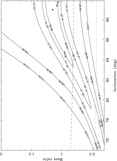
Figure 5: A contour map of the $\chi^{2}$ values is shown (for 100 data bins). The filled circle marks the point with the lowest $\chi^{2}$ value ($\chi^{2}_{\rm min}=94.84$ at $i=89.0^{\circ}$ and $Q=1.15$). The contour levels shown are for $\chi^{2}=\chi^{2}_{\rm min}+1$, $\chi^{2}_{\rm min}+2.30$, $\chi^{2}_{\rm min}+6.17$, $\chi^{2}_{\rm min}+11.8$, and $\chi^{2}_{\rm min}+18.4$. The latter four contour levels correspond to confidence levels of 68.3, 95.4, 99.73 and 99.99 per cent for two parameters of interest. W-D solutions with mass ratios below the dash-dotted line have $M_{\rm total}>1.4\,M_{\odot}$, while solutions with mass ratios below the dotted line have $M_{\rm WD}>1.4\,M_{\odot}$.

With the 7.8 hour modulation removed from the time series data, it was possible to properly analyze the ellipsoidal light curve shown in Figure 4. We modelled the folded light curve using “mode 2” of the W-D code, which is the usual mode used for detached binaries. We assumed a circular orbit and synchronous rotation. The polar temperature of the sdB star was fixed at the spectroscopically determined value of 25,000 K (KOW), and we used coefficients appropriate for the linear cosine limb darkening law taken from the tables of Van Hamme (1993). The gravity darkening exponents for both stars were set to 1, the usual values for stars with radiative envelopes (e.g. Wilson & Devinney 1971 and cited references). [In this particular case, the maximum temperature change over the star is about 4 per cent. Although we do not expect a gravity darkening exponent different than 1, our fits are not sensitive to small changes ($\la 10$ per cent) in this parameter.] Similarly, the bolometric albedos for reflective heating and re-radiation were also set to 1. (We note that there is virtually no “reflection effect” in KPD 0422+5421 since the sdB star is more than 5.5 mag more luminous than the white dwarf. Hence our fits are not sensitive to the exact details of the reflection effect computations.) The free parameters in the model were the inclination $i$, the mass ratio $Q\equiv M_{\rm WD}/M_{\rm sdB}$, the surface potentials $\Omega_{\rm sdB}$ and $\Omega_{\rm WD}$, and the polar temperature of the white dwarf $T_{\rm pole}$(WD).

The “grid size integers” used were $n_{1}=220$ and $n_{2}=20$. A large value of $n_{1}$ was needed to obtain a smooth light curve near phase 0.0, when the white dwarf passes in front of the sdB star. Thus it was necessary to change an input format statement in the W-D code. In that same vein, we also altered the appropriate input format statement to allow for $\Omega_{\rm WD}$ values greater than 99.9999.

Table 1: Parameters for KPD 0422+5421

Parameter	Value with no	Value with white	Reference
	added constraints	dwarf mass-radius constraint
Orbital Period (days)	$0.09017945\pm(1.2\times 10^{-7})$	same	This work
$T_{0}$(photo)	HJD 2,451,$174.493408\pm 0.000057$	same	This work
$K_{\rm sdB}$ velocity (km s${}^{-1})$	$237\pm 18$	…	KOW
orbital separation ($R_{\odot}$)	$0.81^{+0.11}_{-0.15}$	$0.853^{+0.002}_{-0.007}$	This work
$i$ (degrees)	$\geq 84.4$	$\geq 85.6$	This work
$Q\equiv M_{\rm WD}/M_{\rm sdB}$	$1.15^{+0.11}_{-0.34}$	$1.07^{+0.09}_{-0.14}$	This work
$\Omega_{\rm sdB}$	$5.75^{+0.27}_{-0.82}$	$5.55^{+0.24}_{-0.30}$	This work
$\Omega_{\rm WD}$	$71.73^{+7.50}_{-28.97}$	$62.81^{+9.65}_{-8.58}$	This work
$T_{\rm pole}$(sdB), spectroscopic (K)	$25,000\pm 1500$	…	KOW
$T_{\rm pole}$(WD), W-D model (K)	$22,600\pm 2600$	same	This work
$M_{\rm sdB}$ ($M_{\odot}$)	$0.36^{+0.37}_{-0.16}$	$0.511_{-0.050}^{+0.047}$	This work
$M_{\rm WD}$ ($M_{\odot}$)	$0.47^{+0.18}_{-0.16}$	$0.526^{+0.033}_{-0.030}$	This work
total mass ($M_{\odot}$)	$0.86^{+0.52}_{-0.35}$	$1.026_{-0.036}^{+0.079}$	This work
$R_{\rm sdB}$, polar ($R_{\odot}$)	$0.17^{+0.05}_{-0.02}$	$0.193^{+0.009}_{-0.008}$	This work
$R_{\rm WD}$, polar ($R_{\odot}$)	$0.013^{+0.004}_{-0.002}$	$0.0145^{+0.0007}_{-0.0007}$	This work
$\log g_{\rm sdB}$, W-D model (cgs)	$5.55^{+0.06}_{-0.05}$	$5.565^{+0.012}_{-0.006}$	This work
$\log g_{\rm sdB}$, spectroscopic (cgs)	$5.4\pm 0.1$	…	KOW
Note: All errors quoted are 68 per cent confidence.

4.2 Model optimization

We used three types of optimization schemes to fit the light curves, a routine adapted from Bevington (1969) based on the Levenberg-Marquardt scheme, the “grid search” routine adapted from Bevington (1969), and the “differential corrections” program supplied with the W-D code. In our experience a “brute force” procedure of searching parameter space is needed to reliably find the global $\chi^{2}$ minimum, rather than just a local minimum. We began by using several different initial guesses of parameter values for the Levenberg-Marquardt optimization routine, including the parameters found by KOW, and found a set of parameter values that gave a relatively small value of $\chi^{2}$. At this point it became apparent that the overall light curve is insensitive to the value of the polar temperature of the white dwarf–changing $T_{\rm pole}$(WD) only results in a change of the depth of the feature near phase 0.5. We therefore fixed $T_{\rm pole}$(WD) at its optimal value of 24,300 K, leaving four free parameters. Next, we defined a grid of values in the inclination-mass ratio plane covering a range of $75\leq i\leq 90^{\circ}$ in steps of $0.1^{\circ}$ and $0.30\leq Q\leq 2.00$ in steps of 0.1. We started at the point in the $i-Q$ plane corresponding to the provisional solution found above ($i=82.6^{\circ}$ and $Q=0.76$) and the routine was run at each point on the grid. For these fits, the values of $i$ and $Q$ were fixed at the values corresponding to the grid location, leaving only the two surface potentials as free parameters. The grid search routine was then used to optimize the $\Omega$s. Figure 5 shows a contour map of the $\chi^{2}$ values. We found the minimum $\chi^{2}$ value of $\chi^{2}_{\rm min}=94.84$ for 100 data points occurred at the point $i=89.0^{\circ}$ and $Q=1.15$, relatively far from our provisional fit found above. The standard deviation of the residuals (i.e. the data minus the model fit) is 0.002 mag, which is comparable to the statistical errors of the points in the binned light curve.

Our values of $i=89.0^{\circ}$ and $Q=1.15$ are significantly different from the values of $i=78.05\pm 0.50^{\circ}$ and $Q=0.87\pm 0.15$ found by KOW. We believe our present results are more reliable than those of KOW for two reasons. First, we have $\approx 36.6$ hours of CCD observations from a 2.1m telescope (of which $\approx 8.2$ hours was spent reading out the CCD), compared to 7.9 hours of observations obtained by KOW using a high-speed photometer on a 2.1m telescope. Hence our statistics will be better. Second, our CCD data are more reliable since we were able to identify and remove the extra 7.8 hour modulation. KOW were unaware of the extra 7.8 hour modulation, and as a result their folded $U$ and $B$ light curves are likely to be biased and not accurately representative of the true ellipsoidal light curves.

4.3 Computation of parameter uncertainties

Figure 6: Top: The marginal distribution of the values for the total mass as generated using the Monte Carlo procedure. The dashed-dotted lines indicate the region that contains 68 per cent of the area and the dotted lines indicate the region that contains 90 per cent of the area. Bottom: Similar to the top, except the marginal distribution of the values for the sdB mass is displayed.

We used a Monte Carlo procedure to compute confidence limits on the fitted and derived parameters. At each point in the $i$-$Q$ plane shown in Figure 5 we have fitted values of $\Omega_{\rm sdB}$ and $\Omega_{\rm WD}$ and a $\chi^{2}$ of the fit. (The fitted values of the $\Omega$s are basically independent of the inclination and hence are only a function of the mass ration $Q$–larger values of $Q$ result in larger values for both $\Omega_{\rm sdB}$ and $\Omega_{\rm WD}$.) One can define a region in the plane corresponding to a certain confidence limit based on the change in the $\chi^{2}$ values, i.e. the 68 per cent confidence region is defined by $\chi^{2}=\chi^{2}_{\rm min}+2.34$. We divided up the plane into 50 regions with region 1 corresponding to confidence limits between 0 and 2 per cent ($\chi^{2}_{\rm min}\leq\chi^{2}\leq\chi^{2}_{\rm min}+0.041$), region 2 corresponding to confidence limits between 2 and 4 per cent ($\chi_{\rm min}+0.041<\chi^{2}\leq\chi^{2}_{\rm min}+0.081$), and so on. The confidence limits defining the last region were 98 per cent and 99.99 per cent, or $\chi_{\rm min}+7.82\leq\chi^{2}\leq\chi^{2}_{\rm min}+18.43$. Then $2000$ random $i$,$Q$ pairs were selected from each region and the $\Omega$ values were determined using a two-dimensional cubic spline interpolation routine (Press et al. 1992). Finally, for each $i$,$Q$ pair, 10 values each of the mass function and orbital period were drawn randomly from appropriate Gaussian distributions and the system properties (i.e. component masses, orbital separation, etc.) were computed. Confidence limits on the parameters were computed from the marginal distributions of each parameter. Figure 6 shows the frequency distributions for the total mass and for the sdB mass. The mode of the sdB mass distribution is at $M_{\rm sdB}=0.38\,M_{\odot}$, 68 per cent of the values are in the range $0.22\,M_{\odot}\leq M_{\rm sdB}\leq 0.69\,M_{\odot}$ (the lines denoting the confidence limits intersect the histogram at the same $N$-values), and 90 per cent of the values are in the range $0.15\,M_{\odot}\leq M_{\rm sdB}\leq 1.30\,M_{\odot}$. The corresponding values for the total mass are $M_{\rm total}=0.84\,M_{\odot}$ for the mode, $0.53\,M_{\odot}\leq M_{\rm total}\leq 1.34\,M_{\odot}$ for the 68 per cent confidence interval, and $0.39\,M_{\odot}\leq M_{\rm total}\leq 2.22\,M_{\odot}$ for the 90 per cent confidence interval. Table 1 gives the system parameters for KPD 0422+5421 and their 68 per cent confidence regions.

4.4 Additional astrophysical constraints

The 68 per cent and 90 per cent confidence intervals on the masses are somewhat large, which is not surprising considering the relatively large range of mass ratios allowed by the W-D fits. There are potentially two separate astrophysical constraints we can use to limit the parameter ranges, which we describe below.

4.4.1 The white dwarf mass-radius relation

It is highly likely that the unseen star is a white dwarf, and as such has a maximum allowed mass and a well-defined mass-radius relation. However, the W-D code makes no assumption as to what the nature of the unseen star is. The mass and radius of the unseen star are adjusted as necessary when fitting the light curve. In our particular situation, $\Omega_{\rm WD}$ is positively correlated with $Q$. Since the mass of the white dwarf is inversely correlated with $Q$ and the radius of the white dwarf is inversely correlated with $\Omega_{\rm WD}$, we find that the mass of the white dwarf in the W-D fits is positively correlated with its radius (see the bottom panel of Figure 7). The actual mass-radius relation for white dwarfs is in the opposite sense: the radius of a white dwarf get smaller as its mass gets larger. The form of the mass-radius relation is model dependent, and we used the evolutionary tracks of Althaus & Benvenuto (1997, 1998) and Benvenuto & Althaus (1999). These authors have computed evolutionary tracks for both CO and He white dwarfs using a range of hydrogen envelope masses and for a range of metallicities. For each track, we plot in the lower panel of Figure 7 the radius of the white dwarf as a function of its mass when $T_{\rm eff}\approx 35,000$ K and when $T_{\rm eff}\approx 15,000$ K. Some of the low-mass He models do not get as hot at 35,000 K. In these cases we plot the radius corresponding to the hottest available temperature. The intersection of the theoretical mass-radius band and the W-D model confidence limits is relatively small. The lower envelope of the theoretical mass-radius band intersects the 95 per cent confidence contour at $M_{\rm WD}=0.42\,M_{\odot}$ and the upper envelope intersects the same contour at $M_{\rm WD}=0.64\,M_{\odot}$. W-D fits with $M_{\rm WD}\la 0.4\,M_{\odot}$ or with $M_{\rm WD}\ga 0.7\,M_{\odot}$ can be firmly ruled out since the fitted radii are well outside the theoretical mass-radius band. If we use a “filter” in our Monte Carlo simulation and reject the computed values when the white dwarf mass and radius fall outside the theoretical mass-radius band, we find the following: $M_{\rm sdB}=0.511_{-0.050}^{+0.047}\,M_{\odot}$, $M_{\rm WD}=0.526^{+0.033}_{-0.030}\,M_{\odot}$, and $M_{\rm total}=1.026_{-0.036}^{+0.079}\,M_{\odot}$, 68 per cent confidence, or $M_{\rm sdB}=0.511_{-0.066}^{+0.086}\,M_{\odot}$, $M_{\rm WD}=0.526_{-0.040}^{+0.056}\,M_{\odot}$, and $M_{\rm total}=1.026_{-0.049}^{+0.105}\,M_{\odot}$, 90 per cent confidence. The mass of the sdB star is quite consistent with the “canonical” extended horizontal branch mass of $0.5\,M_{\odot}$ (Caloi 1989; Dorman, Rood, & O’Connell 1993; Saffer et al. 1994). Furthermore, the total mass of the system appears to be well below $1.4\,M_{\odot}$. We list in Table 1 the values of the derived parameters (with 68 per cent confidence limits) when the mass-radius constraint is imposed.

Figure 7: Bottom: A contour plot of the two-dimensional frequency distribution of the radius of the white dwarf vs. its mass. The contour levels indicate the regions that contain 68 per cent of the volume and 95 per cent of the volume. The star marks the mode. We also show the theoretical mass-radius relation, taken from the models of Althaus & Benvenuto (1997, 1998) and Benvenuto & Althaus (1999). The filled circles are for CO white dwarfs with $15,000~{}{\rm K}\leq T_{\rm eff}\leq 30,000~{}{\rm K}$ and with various hydrogen envelope masses and the filled triangles are for He white dwarfs. The vertical dashed-dotted lines indicate roughly where the upper and lower envelopes intersect the 95 per cent confidence contour. Top: A contour plot of the two-dimensional frequency distribution of the mass of the sdB star vs. the mass of the white dwarf. The 68 per cent and 95 per cent confidence regions are displayed. The diagonal solid line indicates $M_{\rm WD}+M_{\rm sdB}=1.4\,M_{\odot}$.

It is quite clear that imposing the white dwarf mass-radius constraint greatly reduces the uncertainties on the derived parameters. Although the form of the mass-radius relation is model dependent, the constraint is fairly robust since the theoretical mass-radius band is nearly perpendicular to the ridge-line of points derived from the W-D fits and Monte Carlo simulation. In addition, we have used models with a wide range of hydrogen envelope masses and metallicities, and we have also used a generous range of temperatures (15,000-35,000 K).

As an aside, we can use the Althaus & Benvenuto models to estimate the cooling age of the white dwarf. Each Althaus & Benvenuto model gives the mass, radius, and temperature of the white dwarf as a function of the cooling age. For models where $0.50\,M_{\odot}\leq M_{\rm WD}\leq 0.56\,M_{\odot}$, $0.0138\,M_{\odot}\leq R_{\rm WD}\leq 0.0152\,M_{\odot}$, and $20,000~{}{\rm K}\leq T_{\rm eff}\leq 25,200$ K (i.e. the 68 per cent confidence ranges), we find a range of cooling ages between 11.3 and 50.1 million years. The fact that the white dwarf appears to be relatively young may put constraints on how the present-day binary formed. For example, if the white dwarf formed first, then the second star would have had $\la 50$ million years additional time to evolve into the sdB star, assuming the white dwarf has not somehow been heated since its formation.

4.4.2 The radius of the sdB star

For the second method to potentially reduce the parameter space found by the W-D fits we can exploit the fact that the mass of the sdB star is strongly correlated with its radius ($\Omega_{\rm sdB}$ is positively correlated with $Q$). Hence, the observed rotational velocity of the sdB star will be correlated with its radius. One must assume a rotational period for the sdB star, however. The usual assumption for close binary stars is that $P_{\rm rot}=P_{\rm orb}$, i.e. synchronous rotation, although this may not necessarily be the case (see below). If the rotation is synchronous, then $V_{\rm rot}\sin i=80$ km s^-1 when $M_{\rm sdB}=0.2\,M_{\odot}$ and $V_{\rm rot}\sin i=125$ km s^-1 when $M_{\rm sdB}=0.7\,M_{\odot}$, where the values are computed without using the white dwarf mass-radius constraint. Thus a measurement of $V_{\rm rot}\sin i$ to better than $\approx 10$ km s^-1 would allow one to reduce the available parameter space for the mass of the sdB star. The surface gravity computed from the W-D fits is also correlated with the computed mass of the sdB star. We find $\log g=5.46$ (cgs) when $M_{\rm sdB}=0.2\,M_{\odot}$ and $\log g=5.59$ (cgs) when $M_{\rm sdB}=0.7\,M_{\odot}$, again where the values are computed without using the white dwarf mass-radius constraint. A spectroscopic measurement of $\log g$ is model dependent and requires high quality data (one slight advantage of using $\log g$ to constrain the range of sdB masses is that one does not need to assume a rotational period for the sdB star). Unfortunately, the spectroscopic measurement given by KOW of $\log g=5.4\pm 0.1$ does not provide a definitive answer. The $2\sigma$ range covers nearly all of the $\log g$ range of the W-D fits and Monte Carlo simulation.

4.5 A refined orbital ephemeris

The more precisely defined eclipse profiles also allow us to determine the orbital phase much more accurately. The differential corrections routine of the W-D code can be used to determine the optimal phase (relative to some assumed time) and its probable error. The heliocentric time of the superior conjunction of the sdB star is given in Table 1. The formal $1\sigma$ error on this time is 4.9 seconds, compared with the error of 43 seconds on that measurement given in KOW. Our determination of the phase combined with KOW’s determination leads to the improved measurement of the orbital period given in Table 1.

The accuracy with which we can determine the orbital phase allows for the possibility of measuring the change in the binary period. A possible cause of a change in the orbital period would be the loss of orbital angular momentum via the radiation of gravitational waves. Ritter (1986) gives the period derivative due to gravitational wave radiation as

$$\dot{P}_{\rm GR}=-2.18\times 10^{-14}M_{\rm sdB}M_{\rm WD}(M_{\rm sdB}+M_{\rm WD})^{-1/3}P^{-5/3}$$ (16)

where the masses are in solar masses and the period is in days. Using the masses computed using the white dwarf mass-radius constraint and $P$ given in Table 1 we find $\dot{P}_{\rm GR}=-(3.1^{+0.4}_{-0.2})\times 10^{-13}$. The phase difference $\Delta\phi_{o-c}$ which accumulates over $N$ orbital cycles between the observed orbital phase and the expected orbital phase based on a constant period is $\Delta\phi_{o-c}\approx 0.5\dot{P}N^{2}$ (Ritter 1986). In ten years (40,502 orbital cycles) the accumulated shift will be $\approx 2$ seconds. The formal $1\sigma$ error of our present phase determination is 4.9 seconds. One would need more than twenty years of phase measurements to begin to detect a marginal phase shift, assuming future measurements of the phase have similar uncertainties as ours. The phase might be more precisely determined if the ingress and egress portions of the eclipse profiles were better resolved, although this would be a somewhat daunting task as the white dwarf takes only $\approx 45$ seconds to move a distance equal to its diameter. Nevertheless, a measurement of $\dot{P}_{\rm GR}$ would be valuable since it would provide an independent constraint on the total mass of the system. This assumes that there is no other mechanism acting to remove orbital angular momentum. Note that evolutionary changes of radius of the sdB star on a $10^{8}$ year time-scale might lead to a $\dot{P}$ term of similar size to $\dot{P}_{\rm GR}$, if a small portion of the total angular momentum of the binary is stored in synchronized rotation of the sdB star.

5 Possible Sources of the 7.8 hour Modulation

What is the physical cause of the 7.8 hour modulation which we assert is real? The white dwarf is too faint to account for the 7.8 hour modulation since the depth of the white dwarf eclipse is 0.006 mag whereas the range of the 7.8 hour modulation is $\approx 0.02$ mag from minimum to maximum. Hence the extra (non-ellipsoidal) light must be from the sdB star. We discuss a few possibilities below.

5.1 Star spots?

One possibility is that the 7.8 hour modulation is due to a spot on the sdB star that rotates in and out of view. In this case, the rotational velocity of the sdB star would be substantially slower than the velocity if it were in synchronous rotation: $V_{\rm rot}\approx 28$ km s^-1 compared with $V_{\rm rot}=100$ km s^-1 for synchronous rotation. It should be straightforward to obtain a high resolution spectrum of KPD 0422+5421 and measure the rotational broadening to see whether the measured rotational velocity is consistent with synchronous rotation (the resolution of KOW’s spectrum was not sufficient to place any meaningful constraints on $V_{\rm rot}$).

The W-D fits we have computed all assume synchronous rotation. The W-D code allows one to compute models when $P_{\rm rot}\neq P_{\rm orb}$. We computed a series of W-D models with the “$f_{1}$” parameter set to 2.16/7.8=0.277. The best-fitting model had $i=89.0^{\circ}$, $Q=1.19$, and $\chi^{2}=94.83$. The $\chi^{2}$ contours in the $i$-$Q$ plane looked similar to the contour plot shown in Figure 5. Hence our results are insensitive to changes in the rotational period of the sdB star. We also experimented with “spot” models in the following way: We added a spot to the sdB star and computed several orbital cycles in an attempt to mimic the time series displayed in Figure 1. Each model time series was detrended (using an unspotted model) to isolate the underlying spot modulation. We found that we could not get a modulation with a form matching the shape of the modulation shown in Figure 3 using a single spot. Several spots of various sizes placed at strategic locations on the star may be needed to produce the “sawtooth” pattern that we observe. Until a definitive measurement of $V_{\rm rot}\sin i$ is made that demonstrates $P_{\rm rot}\approx 7.8$ hours (i.e. $V_{\rm rot}\sin i\approx 28$ km s^-1 rather than $\approx 100$ km s^-1 expected for synchronous rotation), a more thorough exploration of spot models does not seem warranted at this time.

5.2 Pulsation?

Another possibility is that the modulation could be due to a pulsational instability in the sdB star. Recently, a new subclass of sdB stars known as the EC 14026 stars has been identified (Kilkenny et al. 1997; Koen et al. 1997; Stobie et al. 1997; O’Donoghue et al. 1997). The EC 14026 stars show modulations with amplitudes of $\la 0.01$ mag and periods of $\la 400$ seconds. In a few cases, these modulations have been identified with low-order radial and non-radial $p$ and $f$ pulsation modes (Billéres et al. 1997, 1998). Many, but not all, of the EC 14026 stars have detectable main sequence companions (e.g. Kilkenny et al. 1998 and cited references). One system, PG 1336-018, is in a HW Vir type binary with an orbital period of 0.10 days (Kilkenny et al. 1998). It is not clear whether the other EC 14026 binaries are astrophysically “close” (periods less than a few days) or “wide” (separations of greater than a few AU).

KPD 0422+5421, with $T_{\rm eff}\approx 25,000$ K is much cooler than the EC 14026 stars ($30,000~{}{\rm K}\la T_{\rm eff}\la 35,000~{}{\rm K}$, Billeres et al. 1997, 1998). Although the amplitudes of the modes observed in the EC 14026 stars are similar to what we observe in KPD 0422+5421, the periods are much shorter. Also, the pulsations observed in the EC 14026 stars have waveforms that are more sinusoidal, rather than the sawtooth pattern we observed. Thus if KPD 0422+5421 is indeed a pulsator, it probably would be in a different class than the EC 14026 stars.

Whatever its cause, the 7.8 hour modulation we observe in KPD 0422+5421 appears to be unique among sdB stars. However, we should note an important point. It is often the case that in reducing high-speed photometry, long term trends (e.g. timescales of hours) are typically removed using polynomial prewhitening or other techniques (C. Koen, private communication). Thus we encourage observers to reexamine their existing data and to acquire additional data. If the 7.8 hour modulation is a real feature of KPD 0422+5421, then our observation should be repeatable if given enough care. If the 7.8 hour modulation is not real, or not strictly periodic, than that too will become evident with additional data.

6 Summary and suggested Future Observations

We have presented additional and extensive CCD observations of KPD 0422+5421. We have discovered that the light curve of this binary star contains two distinct signals, the 2.16 hour ellipsoidal modulation and a non-sinusoidal modulation at 7.8 hours. This extra modulation appears to be intrinsic to KPD 0422+5421 and is not an artifact of the observation or analysis. We removed this 7.8 hour modulation from the light curve and folded the detrended curve on the orbital period to obtain the underlying ellipsoidal light curve. This folded light curve now clearly shows the signature of the transit of the white dwarf across the face of the sdB star and the signature of the total eclipse of the white dwarf (although the latter feature is somewhat noisier than the former feature). We modelled the ellipsoidal light curve with the W-D code and derived values of the inclination, the mass ratio, and the $\Omega$ potentials, and used a Monte Carlo code to compute the uncertainties in the parameters. The marginal distributions of the component masses as computed with the Monte Carlo code have large “tails”, hence the parameters have relatively large uncertainties. If we apply an additional constraint and require the white dwarf’s radius and mass to be consistent with the theoretical mass-radius relation, we find the derived system parameters have much smaller uncertainties. Using the white dwarf mass-radius constraint we find that the mass of the sdB star is somewhat lower than the value determined KOW and is much closer to the “canonical” mass for extended horizontal branch stars. The total mass of the system appears to be less than $1.4\,M_{\odot}$ with high confidence (99.99 per cent). We also find that the white dwarf is much hotter (and hence much younger) than found by KOW. The resolved eclipse profiles allow us to determine the phase accurately, which in turn may allow for the measurement of the orbital period derivative after a reasonable amount of time.

Our basic picture of the KPD 0422+5421 binary is secure, i.e. it contains an sdB star with a mass close to $0.5\,M_{\odot}$ paired with a nearly equally massive white dwarf. Additional spectroscopic observations should be done to improve the determination of the velocity amplitude of the sdB star, to determine its rotational velocity, and to refine the measurements of its effective temperature, surface gravity, and metallicity (a good measurement of the He abundance is needed for a precise determination of $\log g$). An improved $K$-velocity for the sdB star would result in a more precisely determined mass function, which in turn would result in better determined masses. Accurate values of $V_{\rm rot}\sin i$ and $\log g$ could be used to reduce the uncertainty in the mass of the sdB star, independent of the white dwarf mass-radius relation. Further photometric observations should be done in several colours to verify that the 7.8 hour modulation is coherent and to see if its character depends on the bandpass, to better sample the ingress and egress phases of the eclipse profiles, and to provide additional phase determinations so that the change in the period can be tracked over time.

References

- [1997] Althaus L. G., Benvenuto O. G., 1997, ApJ, 477, 313
- [1998] Althaus L. G., Benvenuto O. G., 1998, MNRAS, 296, 206
- [1999] Benvenuto O. G., Althaus L. G. 1999, MNRAS, 303, 30
- [1969] Bevington P. R., 1969, Data Reduction and Error Analysis for the Physical Sciences, McGraw Hill, New York
- [1999] Billéres M., Fontaine G., Brassard P., Charpinet S., Liebert J. Saffer R. A., Vauclair G., 1997, ApJ, 487, L81
- [1999] Billéres M., Fontaine G., Brassard P., Charpinet S., Liebert J. Saffer R. A., Bergeron P., Vauclair G., 1998, ApJ, 494, L75
- [1999] Caloi V., 1989, A&A, 221, 27
- [1999] Dorman B., Rood R. T., O’Connell R. W., 1993, ApJ, 419, 596
- [1999] Downes R. A., 1986, ApJS, 61, 569
- [1999] Frandsen S., Balona L. A., Viskum M., Koen C., Kjeldsen H., 1996, A&A, 308, 132
- [1999] Kilkenny D., Koen C., O’Donoghue D., Stobie R. S., 1997, MNRAS, 285, 640
- [1999] Kilkenny D., O’Donoghue D., Koen C., Lynas-Gray A. E., van Wyk F., 1998, MNRAS, 296, 329
- [1999] Koen C., Kilkenny D., O’Donoghue D., van Wyk F., Stobie, R. S., 1997, MNRAS, 285, 645
- [1999] Koen C., Orosz J. A., Wade R. A., 1998, MNRAS, 300, 695 (KOW)
- [1999] Landolt A. U., 1992, AJ, 104, 340
- [1999] O’Donoghue D., Lynas-Gray A. E., Kilkenny D., Stobie R. S., Koen C., 1997, MNRAS, 285, 657
- [1992] Press W. H., Teukolsky S. A., Vetterling W. T., Flannery B. P., 1992, Numerical Recipes in FORTRAN: The Art of Scientific Computing, Second Edition, Cambridge University Press, Cambridge
- [1999] Ritter H., 1986, A&A, 169, 139
- [1999] Saffer R. A., Bergeron P., Koester D., Liebert J., 1994, ApJ, 432, 351
- [1999] Stellingwerf R. F., 1978, ApJ, 224, 953
- [1999] Stetson P. B., 1987, PASP, 99, 191
- [1999] Stetson P. B., 1990, PASP, 102, 932
- [1999] Stetson P. B., Davis L. E., Crabtree D. R., 1991, in “CCDs in Astronomy,” ed. G. Jacoby, ASP Conference Series, Volume 8, page 282
- [1999] Stetson P. B., 1992a, in “Astronomical Data Analysis Software and Systems I,” eds. D. M. Worrall, C. Biemesderfer, & J. Barnes, ASP Conference Series, Volume 25, page 297
- [1999] Stetson P. B., 1992b, in “Stellar Photometry–Current Techniques and Future Developments,” IAU Coll. 136, eds. C. J. Butler, & I. Elliot, Cambridge University Press, Cambridge, England, page 291
- [1999] Stobie R. S., Kawaler S. D., Kilkenny D., O’Donoghue D., Koen C., 1997, MNRAS, 285, 651
- [1999] Wilson R. E., Devinney E. J., 1971, ApJ, 166, 605 (W-D)
- [1999] Van Hamme W., 1993, AJ, 106, 2096