A Keck High Resolution Spectroscopic Study of the Orion Nebula Proplyds

W. J. Henney Instituto de Astronomía, Universidad Nacional Autónoma de México, J. J. Tablada 1006, Lomas de Santa María, 58090 Morelia, Michoacán, México; will@astrosmo.unam.mx will@astrosmo.unam.mx C. R. O’Dell Department of Space Physics and Astronomy, MS-108, Rice University, P.O. Box 1892, Houston, TX 77251; cro@rice.edu cro@rice.edu

(Accepted by The Astronomical Journal 29 July 1999 (in press November 1999))

Abstract

We present the results of spectroscopy of four bright proplyds in the Orion Nebula obtained at a velocity resolution of 6 km s^-1. After careful isolation of the proplyd spectra from the confusing nebular radiation, the emission line profiles are compared with those predicted by realistic dynamic/photoionization models of the objects. The spectral line widths show a clear correlation with ionization potential, which is consistent with the free expansion of a transonic, ionization-stratified, photoevaporating flow. Fitting models of such a flow simultaneously to our spectra and HST emission line imaging provides direct measurements of the proplyd size, ionized density and outflow velocity. These measurements confirm that the ionization front in the proplyds is approximately D-critical and provide the most accurate and robust estimate to date of the proplyd mass loss rate. Values of $0.7\mbox{--}1.5\times 10^{-6}\mbox{M}_{\odot}\,\mbox{yr}^{-1}$ are found for our spectroscopic sample, although extrapolating our results to a larger sample of proplyds implies that $0.4\times 10^{-6}\mbox{M}_{\odot}\,\mbox{yr}^{-1}$ is more typical of the proplyds as a whole. In view of the reported limits on the masses of the circumstellar disks within the proplyds, the length of time that they can have been exposed to ionizing radiation should not greatly exceed $10^{4}$ years — a factor of 30 less than the mean age of the proplyd stars. We review the various mechanisms that have been proposed to explain this situation, and conclude that none can plausibly work unless the disk masses are revised upwards by a substantial amount.

Subject headings:

H II regions–ISM:individual(Orion Nebula)–stars:formation

1. Introduction

Thick disks of circumstellar material seem to be an integral and perhaps necessary component of newly formed stars. When these stars are found in or near an H II region the possibilities of their detection and survival become quite different than in regions lacking massive early type stars. The identification of this special class of objects, called the proplyds (O’Dell et al. 1993), was first made in the Orion Nebula, with two more distant objects having been found (Stapelfeldt et al. 1997, Stecklum et al. 1998). The Orion proplyds are bright and have been detected as unresolved stars for many decades; however, their special nature did not begin to become unveiled until the emission line images of Laques & Vidal (1979) showed them to be compact ionized sources. These observations were extended with VLA observations at an angular resolution of 0.1″ (Garay et al. 1987, Churchwell et al. 1987), with the latter paper identifying their correct nature (young stars with circumstellar clouds photoionized from the outside by $\theta^{1}\,$ C Ori) as one of the possible models, a view shared by Meaburn (1988) soon after. However, it was the first HST WFPC2 images in the core of the Orion nebula that clearly revealed the correctness of this interpretation (O’Dell et al. 1993) and showed that the proplyds came in a variety of forms and brightnesses. What one sees depends very much on the location and orientation of the proplyd. Those distant from $\theta^{1}\,$ C Ori and shielded from its ionizing radiation appear dark in silhouette against the bright nebular background, while those close to $\theta^{1}\,$ C Ori have their outer parts ionized by that star. This is revealed by bright cusps on the side facing $\theta^{1}\,$ C Ori, the surface brightness of which scales with distance from the ionizing star in the manner expected (O’Dell 1998). In several of the bright proplyds one can see the inner neutral dust disk in silhouette. In all cases one can see a low mass star at the center of the proplyd, except for two objects whose disk plane lies almost along the line of sight(McCaughrean & Stauffer 1994, O’Dell & Wong 1996, McCaughrean & O’Dell 1996, Chen et al. 1998).

A neutral hydrogen column density of about 10 ${}^{17}\,$ cm^-2 is all that is required to reach an optical depth of unity in the Lyman continuum radiation and thus an ionization front (IF). It is not surprising, therefore, that the bright proplyds are bounded on the side facing the ionizing star by a well defined ionization boundary. That the bright rims are indeed IFs is established not only by the variation of their surface brightness as the inverse square of the distance from $\theta^{1}\,$ C Ori, but also from the fact that this feature is also bright in [O I] and [S II] lines, telltale emission that can only arise in an IF. The most promising explanation for the observed structure of the bright proplyds, is that a dense, slow neutral wind is driven from the (largely molecular) circumstellar accretion disk by the heating effect of non-ionizing FUV radiation. This explanation was initially hinted at by McCullough (1995), but was first developed in depth by Johnstone et al. (1998). The flux of ionizing EUV photons is not sufficient to ionize this wind all the way to its base and so an IF forms that is offset from the disk surface by a few disk radii. At present quite sophisticated models for the proplyds have been generated within this framework (Henney & Arthur 1998, Johnstone et al. 1998, Störzer & Hollenbach 1998,1999), all sharing the features that neutral hydrogen is fed from the disk (where hydrogen exists as H₂, Chen et al. 1998) into an extended outer atmosphere whose side facing $\theta^{1}\,$ C Ori or $\theta^{2}\,$ A Ori is photoionized. The Störzer & Hollenbach (1998,1999) models contain the most detailed treatment of the photodissociated neutral flow and establish that they can explain both the intensity of the H₂ at the boundary of the inner disk and also the [O I] emission that has been observed there (Bally et al. 1998b) and cannot arise from collisional excitation by photoelectrons. Models in which the accretion disk is directly ionized by EUV radiation (Henney et al. 1996, Richling & Yorke 1999) may apply to the smallest proplyds, which are closest to $\theta^{1}\,$ C Ori.

The fact that material should freely flow away from the ionization front (Dyson 1968), hence producing mass loss from the proplyds, was recognized as early as the Churchwell et al. (1987) discovery paper, with current models predicting rates of about 10^-7–10^-6 M ${}_{\hbox{$\odot$}}$ yr^-1. The mass loss rate depends on the IF radius, $r_{0}$ , photoevaporating flow velocity, $u_{0}$ , and peak ionized density, $n_{0}$ , as $(\dot{M}/10^{-7}\mbox{M}_{\odot}\,\mbox{yr}^{-1})\simeq 2\mbox{--}4\,(r_{0}/10^{15}\,\mbox{cm})^{2}(u_{0}/13\,\mbox{km}\,\mbox{s}^{-1})(n_{0}/10^{6}\,\mbox{cm}^{-3})$ . The constant of proportionality in this equation varies according to the relative importance of mass loss from the sides and tails of the proplyds. The masses of the disks can be estimated from thermal emission from their dust component, with the result that the most massive contain about 10^-2 M ${}_{\hbox{$\odot$}}$ (Mundy et al. 1995, Lada et al. 1996, Bally et al. 1998b). Combining these masses with the theoretically predicted mass loss rates, indicates disk destruction times of about a few times 10⁴ to 10⁵ years. Although one knows that the Trapezium Cluster (TC) is quite young (Hillenbrand 1997), the position of the stars on the luminosity versus temperature diagram indicating an age of 300,000 to 10⁶ years, the uncertainties of the pre-main sequence stellar models being used prevents determination of an exact age or identification of an extended period of star formation. In any event, the theoretically predicted disk survival ages are short compared with the age of the cluster, and, furthermore, there is no depletion of proplyds as one samples regions closer to $\theta^{1}\,$ C Ori (O’Dell & Wong 1996, Henney & Arthur 1998). This means that we are missing some ingredient in the modeling. Störzer & Hollenbach (1999) argue that the conundrum can be resolved by assuming that the proplyds are in highly elliptical orbits, thus spending only a small fraction of their time in the vicinity of $\theta^{1}\,$ C Ori. O’Dell (1998) has argued that Ly $\alpha$ photons trapped within the confines of the nebula can produce a sufficent net inward force to stop the proplyd loss of mass, but it should be noted that what he derives as the amount of this constraining pressure would actually be an upper limit. Although there was some hope that one could determine from the HST images whether or not the ionized portions of the proplyds were in static equilibrium, these aspirations were dashed when Henney & Arthur (1998) showed that the nearly exponential surface brightness distributions within the bright cusps could equally well be explained by both a freely expanding and a static atmosphere. This means that one must look to more direct means of determining the mass loss rates.

The most powerful means available is to directly measure the velocity of the flow of material off of the IF of individual proplyds. This approach presents particular observational challenges in obtaining and analyzing the data and demands good supporting theoretical work. The observational challenges are primarily ones of accurately subtracting the high velocity emission from any jets associated with the proplyds and the low velocity background emission from the Orion nebula. Supersonic flows from the proplyds were first detected by Meaburn (1988) in the [O III] 5007Å line, who then characterized them more fully with additional spectra (Meaburn et al. 1993, Massey & Meaburn 1995, Henney et al. 1997). These flows were studied in additional lines by Hu (1996) and the entire nebula was completely covered with Fabry-Perot spectra in [O III] and [S II] (O’Dell, et al. 1997). Sources with known jet flows are to be avoided when looking for the photoevaporative flows, but one does not always know beforehand that they are there. Fortunately the flows are sufficiently large to be separable. Accurate isolation of the proplyd spectrum from the signal that contains both the proplyd and nebular background emission is a greater challenge. Both emissions come from the fluoresence of Lyman continuum photons, with the closer proplyds seeing a higher flux of these photons than the nebular IF, but the proplyds are smaller than the typical seeing disk of a groundbased telescope, so that their signal is often a small fraction of the total signal. Henney et al. (1997) made a thorough analysis of the best proplyd spectra from the Massey & Meaburn (1995) data set and demonstrated that good isolation of velocity components near but not at the systemic velocity could be done. Even if good observational isolation of the spectrum of the proplyd can be obtained, its correct interpretation requires independent knowledge of as many of the proplyd parameters as possible (e. g., ionized density, IF radius, orientation), for which the best images must be employed. Once the spectra are in hand and these parameters determined, then one must have the predicted line profiles that would be expected for the static or freely expanding ionized atmospheres. It is these factors that have guided the formulation of the study reported in this paper.

2. Observations and Data Reduction

The exact determination of the mass loss rates of the proplyds has repercussions that go well beyond whether or not the TC circumstellar disks will survive. The standard paradigm for star formation is that the TC is more characteristic of where the bulk of stars form than less rich clusters such as those found in the Taurus cloud where high mass stars are not found. If the TC is characteristic and the circumstellar disks are rapidly destroyed, it seems unlikely that planet formation will be ubiquitous. It was, therefore, considered worth the time and effort to pursue the question of the proplyd mass loss rate with the most powerful groundbased telescope: the Keck I observatory at Mauna Kea, Hawaii. Fortunately, this opinion was shared by the persons allocating Keck time within the NASA “Origins Program” and the observations were carried out as part of a joint program with John Stauffer, who was studying low mass stars in the same region with the same instrumental configuration.

The observations were made with the Keck I telescope the nights (UT) of 5 and 6 December 1997 using the HIRES spectrograph and a 1024 $\times$ 2048 Tektronix CCD. The entrance slit was 0.862 $\times$ 14″, projecting onto the detector with a velocity resolution of 6.2 $\pm$ 0.4 km s^-1 and a scale of 0.382″/double-binned-pixel perpendicular to the dispersion. The HIRES spectrograph is a cross dispersed echelle spectrograph system used in a configuration such that when the 14″ long slit is used, the ends of the highest orders employed (containing the [O III] 4959Å and the H $\beta$ 4861Å lines) overlapped. Fortunately, the Tektronix CCD has a large linear range and the limiting signal imposed by the digitizing system (2¹⁶=65,536 counts) fell well beneath it. This large dynamic range allowed both strong and weak emission lines to be recorded at a single echelle setting. Wavelength calibration was provided from exposures of a Thorium+Argon standard lamp. Unfortunately, the Tektronix CCD had several pixel defects, whose impact was minimized by adjusting the echelle and cross dispersing grating orientations, but one such defect precluded using the images of the stronger [O III] 5007Å line, which was not a serious problem as the [O III] 4959Å line from the same upper state always provided an adequate signal.

The observing strategy was to select four proplyds which are located in relatively smooth portions of the Orion nebula, are free from adjacent bright stars, and represent a variety of sizes and morphologies. The objects observed were 170–337 (HST2), 177–431 (HST1), 182–413 (HST10), and 244–440. The coordinate based designation system of O’Dell & Wen (1994) will be used throughout this paper, the previous parenthetical designations being those of the serial listing in an earlier paper (O’Dell et al. 1993).¹¹1244–440 was discovered later (O’Dell & Wong 1996), but incorrectly included in their table of stellar objects because its emission line shell was much larger than in any other Orion proplyd. The first three objects have sizes (measured as the distance between their bright cusp tips) of 0.4″, 0.6″, and 1.2″ (O’Dell 1998), while 244–440 is significantly larger, having a similarly measured width of 3.5″. Since the objects all show symmetry to a greater or lesser degree about lines pointed towards their ionizing star ( $\theta^{1}\,$ C Ori for the first three proplyds and $\theta^{2}\,$ A Ori for 244–440), observations were made with position angles along and perpendicular to these lines. Small deviations in angle were made to avoid bright stars and an additional angle was added for 170–337 to lie along the known direction of a microjet and associated shock feature (O’Dell 1998, Bally et al. 1998a). The PA’s used were 151, 231, and 353° for 170–337, 135 and 225° for 177–341, 62 and 152° for 182–413, 52 and 142° for 244–440. The slit PA was held fixed throughout the exposures of 300, 450, and 900 seconds by the Keck I image rotator, whose accuracy was checked using stars of known orientation. The astronomical seeing was typically 1.5″ and the transparency varied from clear to partly cloudy.

Producing easily usable spectra from the complex echelle spectrograms required a series of steps. A 512 pixel long segment centered on the emission line was sampled and the correct echelle order isolated. The spectra in these samples are tilted owing to the use of a cross dispersion. The tilt was removed by using modifications of tasks within IRAF²²2IRAF is distributed by the National Optical Astronomy Observatories, which is operated by the Association of Universities for Research in Astronomy, Inc. under cooperative agreement with the National Science foundation., the result being two dimensional spectra with the calibrated wavelength as the $x$ -axis and the angular position along the slit as the $y$ -axis. These steps were duplicated for each of the following spectral lines: [S II] 6731Å, [N II] 6583Å, H $\alpha$ 6563Å, [S III] 6312Å, [O I] 6300Å, He I 5676Å, [O III] 4959Å, H $\beta$ 4861Å. The [S III] and [O I] lines were sufficiently close that they were processed as a single sample. Radial velocities were calculated using the rest wavelengths employed by Esteban et al. (1998), with the exceptions that a rest wavelength of 6300.31Å was used for [O I] according to the arguments of O’Dell & Wen (1992) and 5875.74 for He I 5676Å, which gives the same velocity as the [O III] lines which should arise from the same emitting layer. In those sections where adjacent spectral orders overlapped there was an enhanced signal due to the continuum of the contaminating order being added to the continuum of the order containing the emission line of interest. This small contamination was subtracted from the region of overlap by appropriate scaling. We made certain that there was no contamination of the subject emission lines by other emission lines in adjacent orders.

3. Data Analysis

The primary challenge in extracting proplyd spectra from groundbased telescope spectrograms is in the accurate subtraction of the nebular background. The peak surface brightness of the proplyds is higher than that of the nebula but at typical ground observatory angular resolutions the image is smeared and the observed surface brightness drops to a value comparable to or less than the background, so that one is extracting a smaller signal from a larger. This problem is compounded by the fact that the nebular background to be subtracted is not homogenous and shows significant variations on scales of several arcseconds. At the signal levels obtained in the present observations the uncertainty due to photon statistics was much smaller than the uncertainties encountered in the background subtraction. Although most of the nebular emission occurs in a small velocity range corresponding to emission from material accelerating away from the main IF, there is considerable information in the line profiles near the systemic velocities, so that accurate correction for the background needs to be made at all velocities. The best previous attempt at extracting proplyd spectra is that of Henney et al. (1997), who obtained profiles of five objects, with only that of 158–323 (LV5) being good enough to make a detailed comparison with the expectations of the models. Even for 158–323 there was considerable uncertainty about the profile near the systemic velocity of the nebula. Moreover, that investigation treated only the [O III] 5007Å line and in only one spectrum for each object. Therefore, it was impossible to quantitatively assess the uncertainties of the extracted profiles. The present data set is much more complete since it looks at emission lines representing a broad range of ionization states and contains multiple spectra taken at a variety of PA’s. The range of ionization states should be useful in the diagnosis of the proplyds and the wealth of spectra should allow determination of the errors that occur because of vagaries in extraction of the background.

Data is not available for all lines in all proplyds. The H $\alpha$ line was saturated in all the long exposures except for 244–440. Some lines are intrinsically weaker and the background less well defined. There was an object-to-object variation in the contrast of the proplyd against the background due to the fact that the brightness of the nebular emission, mainly arising near the IF, varies with angular distance from the photoionizing star in a manner different from that of the proplyds, owing to the different geometrical factors involved. The data set used in the analysis is a subset of the total, our having rejected saturated and low contrast emission lines. Within this subset some portions of the spectra were not used because of the known presence from images of shock or jet features which would have rendered background subtraction more uncertain.

3.1. Subtraction of the nebular background

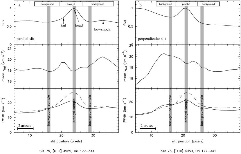
Line profiles of the proplyds were extracted in two quite different fashions, the two methods having their own specific advantages. The first method used larger background samples at slightly greater distances from the proplyd, but employed known surface brightnesses on HST images to scale to the position of the proplyd. The second method relied on a simple subtraction of the background using smaller and slightly closer samples, with the judgement about where the sample should be taken being based on the profile along the slit. Henceforth, these will be referenced as the “large-sample” and the “small-sample” methods. In both methods, the continuum emission (arising from free-free and free-bound processes in the ionized gas plus dust scattering of starlight) was removed from each sample before subtraction. Examples of the samples used in the two methods are shown in Figure 1.

In the “large-sample” method of extraction the characteristic sample size for the proplyd was 3.8″ with background samples of about 2.0″ centered at distances of about 3.0″ from the proplyd. The exact sizes and distances varied according to where the proplyd was located within the entrance slit on a particular spectrum. With the seeing disk size that applied during the observations, these sizes and distances allowed reasonable isolation of the smallest three proplyds, but did sometimes subtract part of the proplyd spectra, this problem being greatest for 244–440. Such partial subtraction should not alter the nature of the resultant profile, only reduce its total signal. Whenever possible, two background samples were taken, one to each side of the proplyd sample, as illustrated in Figure 1. We designate as a single profile the result of subtracting the background based on either of the two background samples, which means that two subtracted profiles could result from a single spectrum. The amount of background signal subtracted was not simply the value in each region, rather, it was this value scaled according to relative surface brightnesses on HST images. We extracted samples of the HST images made in the vicinity of each proplyd in either the same line or a line of similar ionization (O’Dell & Wong 1996) and rotated these samples to have the same orientations as the slits employed. Regions accurately matching the background samples were then identified and measured. For comparison of these background surface brightnesses to that at the proplyd, we then identified and measured rectangular (long axis parallel to the slit) samples close to and on both sides of the proplyd image. The average of those two samples was then taken to be the surface brightness at the proplyd position. The ratio of this value to that of each background sample was then used to scale the background prior to subtraction from the nebula.

The attraction of this method of background subtraction is that it uses the best information in scaling the amount of background subtracted and allows the isolation of the maximum amount of proplyd spectrum. The primary disadvantage of the method is that neither the high, low, or proplyd background samples have been smeared according to the astronomical seeing that applied, which varied from 1 to 2″. The importance of this limitation is revealed in the scatter of profiles obtained using similar sample regions on different spectra.

In an effort to overcome some of the difficulties that arose in the “large-sample” method, a second attempt to extract the line profiles was made using smaller samples (0.4–1.2 $\arcsec$ ). The motivations for choosing small proplyd samples were, firstly, to maximize the ratio of proplyd to nebular emission in the sample, and, secondly, to minimize the contribution of emission from the proplyd tail to the sample. The motivations for choosing small background samples were, firstly, to ease the avoidance of “pathological” regions of the nebula (for example, the bowshock that lies in front of some of the proplyds), and, secondly, to allow the background samples to be as close as possible to the proplyd, thereby minimizing the distance over which the nebular profile need be interpolated. In order to help choose the positions of the samples, graphs were constructed of three parameters of the line profile (total intensity, mean velocity, and velocity width) as a function of position along the slit. An example plot is shown in Figure 1. By means of these and the HST images, samples were chosen covering the peak of the proplyd emission, together with nearby background samples that avoided shocks and other “features” in the nebular background. In this “small-sample” method, no attempt was made to scale the nebular samples using the HST images before subtraction from the proplyd sample.

4. Extracted Proplyd Line Profiles

The proplyd emission line profiles that result from application of the two nebula subtraction methods of the previous section are shown in Figure 2 for the four proplyds 170–337, 177–341, 182–413, and 244–440. Prior to the averaging of the individual extracted profiles discussed in the previous section, these were shifted to a common heliocentric velocity scale and normalized using the wings of the profiles, as far as possible from the velocities showing substantial nebular emission. The resultant averaged extracted profiles are of varying quality. For the proplyds 177–341 and 244–440, the results are very good for all lines, with the two subtraction methods agreeing to within their mutual error bars. For 170–341 and for the high-ionization lines of 182–416, the results are generally poorer. In the case of 170–341, this is mainly because of the strongly fluctuating nature of the background nebular profile at that position, while, in the case of 182–416, it is due to the poor contrast between the proplyd and the nebula, especially in high-ionization lines such as [O III] 4959Å.

The “small-sample” method generally uses a larger number of background samples and often has smaller scatter than the “large-sample” technique. However, we caution that this does not necessarily imply that the results of this method are more reliable. Rather, we take the conservative view that the line profiles can only be fully trusted where the two methods are in agreement.

4.1. Extinction by dust in the proplyd

One unknown factor that may introduce systematic errors in the extracted profiles is the extinction of the background nebular emission by dust in the proplyd. If this were a significant effect it would result in the over-subtraction of the nebular line and could even cause the extracted profile to become negative. It can be seen that for some lines the extracted profile is indeed negative for certain velocity ranges (Fig. 2). However, it is not clear if this is a real effect or merely due to errors in the estimation of the nebular emission at the proplyd position.

HST images of 182–413 show that the circumstellar disk in this object is completely opaque at visible wavelengths (Bally et al. 1998). This disk is much smaller than the seeing disk in the current observations and will reduce the nebular emission at the proplyd position by at most 1% (in the extreme case in which there is no nebular emission from in front of the proplyd), which is much less than the uncertainty due to the spatial variation of the nebular emission.

A potentially more important effect, although one very difficult to quantify, is extinction by dust in the extended neutral envelope of the proplyd and in the ionized photoevaporated flow itself. Even a moderate optical depth here can have a significant effect if the area of the proplyd is comparable to, or greater than, that of the seeing disk, which is certainly the case for 182–413 and 244–440. Henney & Arthur (1998) find hydrogen column densities through the ionized photoevaporated flows in the range $10^{20}$ – $10^{21}\,\mbox{cm}^{-2}$ , while the models of Störzer & Hollenbach (1999) predict column densities through the neutral photoevaporated flows of approximately $5\times 10^{21}\,\mbox{cm}^{-2}$ . Hence, dust in the photodissociated flow inside of the IF will probably be the dominant factor in the extinction of background nebular emission.

If the dust-gas ratio of the grains responsible for the visual extinction is “normal” (corresponding to an extinction cross-section per H atom of $5\times 10^{-22}\,\mbox{cm}^{-2}$ ), then the mean extinction optical depth through the proplyd will be about 4. However, the “effective” extinction will be less than this for three possible reasons. Firstly, apart from 244-440, all the proplyds are smaller than the seeing width (at least across their minor axis), so the extinction will be “diluted” by a factor roughly equal to the ratio of the projected area of the proplyd to the area of the seeing disk. In 177-341, for example, this amounts to about a factor of 3. Secondly, some of the nebula emission may arise in front of, rather than behind, the proplyd, and so will suffer no extinction due to dust in the proplyd. This is unlikely to be an issue for proplyds near $\theta^{1}\,$ C Ori, where the majority of the nebular emission is confined to a thin layer near the principal IF (Baldwin et al. 1991; Wen & O’Dell 1995), but may become important for the more distant proplyds (182–413, 244–440). Thirdly, the nebula subtends a large solid angle as seen from the proplyds and so, for reasonable values of the dust albedo and scattering phase function, scattering into the line of sight will be important (Henney 1998), possibly reducing the effective extinction by a factor of 2 or more. Furthermore, there exists the possibility that the grains responsible for producing the visual extinction will be selectively depleted in the proplyd photoevaporating flows. As noted by Hollenbach, Yorke & Johnstone (1999), theories of dust settling and coagulation in disks (Weidenschilling 1984; Weidenschilling & Cuzzi 1993) imply that larger grains settle to the disk midplane more rapidly than smaller grains, where they will coagulate into larger bodies. Hence, it may be that the $\sim 0.1\mu{\rm m}$ grains responsible for the visual opacity are depleted in the neutral flow from the circumstellar disk, whereas the $\sim 0.01\mu{\rm m}$ grains responsible for the FUV opacity are not.

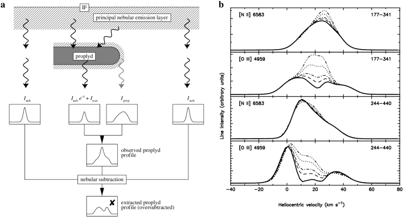
Figure 3 shows examples of the effects on the subtracted line profiles of different degrees of extinction of the background nebula by dust in the proplyd. The thick lines show the line profile assuming that the proplyd is totally transparent (as in Fig. 2) while the thin lines show the effect of assuming an effective extinction, $A_{V}$ , in the range 0.1–1.0. It can be seen that the [N II] lines in the two proplyds shown are hardly affected by the assumed value of $A_{V}$ , whereas the [O III] lines are affected substantially. This is partly due to the difference in wavelength between the two lines ([O III] is bluer, and so suffers greater extinction for a given $A_{V}$ ), but mainly due to the fact that relative brightness of the proplyds compared to the nebula is greater in [N II] than in [O III]. The apparent minimum at the center of the [O III] lines is seen to disappear for $A_{V}\geq 0.2$ , and so its real existence is doubtful. On the other hand, it seems that $A_{V}$ cannot be much greater than 0.5, since at this level of assumed extinction the nebular line starts to show through clearly in the extracted profile, implying that the background has been undersubtracted.

Studies of the spatial and velocity variations in the H $\alpha$ /H $\beta$ ratio (Henney & Watson 1999) are consistent with an effective extinction of $A_{V}=$ 0.1–0.2 in the proplyds, although the exact amount is uncertain because of possible deviations from Case B emissivity. It remains to be seen whether or not such a low value can be reconciled with the expected column densities in the photodissociated flows without invoking selective depletion of the grains.

4.2. Parameters of the extracted line profiles

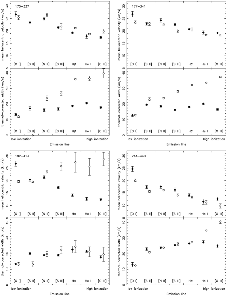
Figure 4 shows the mean velocity and widths of all the extracted proplyd spectra (open symbols), together with the same quantities for the adjacent background nebula samples (filled symbols). The flux-weighted mean velocity of a line profile $I(v)$ is given by

\bar{v}=\int_{-\infty}^{\infty}vI(v)\,dv\ \Bigg{/}\int_{-\infty}^{\infty}I(v)\,dv\ .

For the line width, we use the quantity $2.355\,\sigma$ , where $\sigma$ is the flux-weighted RMS width of the line, given by

\sigma=\left[\int_{-\infty}^{\infty}(v-\bar{v})^{2}I(v)\,dv\ \Bigg{/}\int_{-\infty}^{\infty}I(v)\,dv\right]^{1/2}\ .

For a Gaussian line profile, $2.355\,\sigma$ is equal to the FWHM of the line. However, the line profiles are often very non-Gaussian, both for the proplyds and for the background nebula. In such cases, $\sigma$ is a more robust estimate of the line width than the FWHM, especially when the line is double-peaked.

The line widths have been corrected for the effects of thermal and instrumental broadening by quadrature subtraction of the widths of the respective profiles. The instrumental width is approximately 6 km s^-1 and an ion kinetic temperature of $8900\,$ K was assumed in all cases, corresponding to a thermal width of 20 km s^-1 for the hydrogen lines. The lines are arranged in order of increasing ionization potential (IP), ranging from [O I] 6300Å, which is expected to come from neutral gas, to He I 5676Å and [O III] 4959Å, which should come from the most highly ionized gas in the H II region.

4.2.1 Trends in the lines from the background nebula

The mean velocities of the nebular lines show a clear trend of increasing blueshift with IP, as first reported by Kaler (1967). This trend is commonly interpreted as being due to an ionization stratification in the nebula (more highly ionized species are found closer to the ionizing star), coupled with an acceleration of gas away from the ionization front (which is seen close to face-on).³³3One slight inconsistency of our data with this picture is that [S II] is always blueshifted by 1–2 km s^-1 with respect to [N II]. This is the reverse of what is expected since the ionization potentials of S⁰ (10.36 eV) and S⁺ (23.33 eV) are much lower than those of N⁰ (14.53 eV) and N⁺ (29.60 eV), implying that the [S II] emission should arise from partially ionized regions (the IF itself and the neutral photodissociation region), whereas the [N II] emission should come mainly from the H⁺/He⁰ zone. This discrepancy could be resolved if the rest wavelength of one or other of the two lines were in error by $0.02$ Å, which is well within the uncertainty of the determination of the rest wavelengths. Such a scenario (Zuckerman 1973), in which the majority of optical line emission at small angular displacements ( $<2\arcmin$ ) comes from a thin layer close to the IF on the surface of the background molecular cloud, has been shown to be broadly consistent with a mass of observational material (e.g. Baldwin et al. 1991; O’Dell et al. 1993a; Wen & O’Dell 1995). However, a detailed physical model is still lacking.

The thermal-corrected width of the nebular emission lines does not seem to vary significantly with IP, except for [O I] 6300Å, which is consistently narrower. However, the width does vary substantially from position to position, being much larger at the position of 244–440. It should be noted that the widths given here are for the line as a whole, rather than for individual Gaussian components, as have been used in some previous studies (Castanẽda 1988; O’Dell & Wen 1992; Wen & O’Dell 1993).

4.2.2 Trends in the lines from the proplyds

For three of the four proplyds, the mean velocities of the extracted lines follow the same general trend as the nebular lines, but with the pattern shifted 1–2 km s^-1 to the blue (177–341 and 244–440) or to the red (170–337). There is also a tendency for the velocity gradient to be shallower for the proplyds than for the background nebula. For 182–413, on the other hand, the trend is in the opposite direction (lines from more highly ionized species are more redshifted). For all objects except 170–337 the proplyd [O I] 6300Å line is significantly blueshifted by 3–7 km s^-1 with respect to the nebula. Possible explanations for this are outlined in section 8.2.3.

The thermal-corrected width of the extracted proplyd lines is perhaps the most interesting and important property plotted in Figure 4. In marked contrast to the behaviour of the background nebular lines, the proplyd lines show a strong increase in width with increasing ionization potential. This can be very clearly seen in three of the objects, although it is less apparent in 182–413 because the data for the high ionization lines in this object are very poor due to low contrast against the nebula.

This correlation can be directly understood in terms of ionization stratification in an accelerating photoevaporating flow, in a similar way to the velocity-IP correlation for the nebular lines. There are two differences, however, between the flow from the proplyds and that from the principal IF of the nebula. First, the proplyd flows are much more divergent than the nebular flow, which leads to a more rapid acceleration, especially close to the IF (Henney & Arthur 1998). Second, the proplyds are small compared with the scale of the observations and their neutral portions are at least partially transparent, which means that the observed line profiles come from gas moving in a wide range of directions with respect to the line of sight, both approaching and receding. With the nebula, on the other hand, the line profile from a given point samples only a thin pencil beam through the emitting gas, all of which is probably moving in a similar direction. These are the two reasons why the proplyds show such a spectacular linewidth-IP correlation, while the background nebula does not.

5. Photoevaporating Flow Models

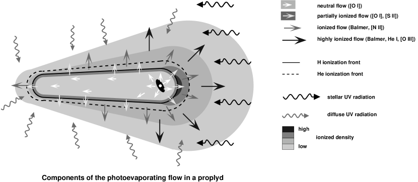
The photoevaporating flow models employed in this work are a development of those presented in Henney & Arthur (1998), building on the previous work of Dyson (1968) and Bertoldi (1989). Figure 5 shows the principal features of the model in schematic form. It is supposed that a strong D or D-critical ionization front (IF) surrounds the proplyd’s neutral envelope (probably a slow photodissociated wind from the circumstellar accretion disk, Johnstone et al. 1998) and that the newly ionized gas flows freely away from the proplyd. The ionization front on the “front” side of the proplyd, which faces the ionizing star, is idealized to be hemispherical and the gas is assumed to flow radially. The ionized gas is assumed to be isothermal, in which case the radial profiles of density and velocity in the flow follow from Bernoulli’s equation. It is found that pressure gradients in the ionized gas cause the flow to accelerate away from the IF, with the acceleration being greatest in the D-critical case (when the flow leaving the IF is exactly sonic). The variation of the density of ionized gas with angle around the IF is calculated assuming ionization equilibrium. The density is highest at the point on the IF closest to the ionizing star (sub-stellar point) and in the simplest case (no dust, no diffuse ionizing field, and few ionizing photons reaching the IF) falls off as $\cos^{1/2}\theta$ , where $\theta$ is the angle between a point on the IF surface and the sub-stellar point. Note that in this approximation the ionized density falls to zero at $\theta=90^{\circ}$ .

The main development of the models with respect to Henney & Arthur (1998) is the treatment of the diffuse ionizing field and the proplyd tails. This work is only summarised here and will be described in greater detail elsewhere (Henney 1999). The diffuse ionizing field in the Orion nebula arises mainly from the radiative recombination of hydrogen to its ground state, with minor contributions from helium recombination and scattering by dust particles. We characterize this diffuse field by the parameter $\beta$ , which denotes the ratio of direct (stellar) to diffuse (nebular) ionizing flux at the proplyd position and we assume that the diffuse field is isotropic. In the case where diffuse ionizing photons are always reabsorbed close to their point of emission (on-the-spot approximation), one finds that $\beta\simeq 0.15$ . However, the mean-free-path of ionizing photons can be very large in the interior of an H II region and simple calculations suggest that $\beta$ should lie in the range 0.01–0.05 at the positions of typical proplyds.⁴⁴4Note, however, that the on-the-spot approximation is employed in treating the diffuse photons emitted in the photoevaporating flow itself. The diffuse ionizing field results in a non-zero value for the density at $\theta=90^{\circ}$ and also allows the ionization of the “back” part of the proplyd, which the front-facing ionization front shadows from direct stellar radiation. This gives rise to the proplyd tails, which in the current models are assumed to be cylindrical, with axis pointing directly away from the ionizing star. The ionized density is calculated as a function of position along the tail, again assuming ionization equilibrium, and simultaneously solving for the radiative transfer of the direct and diffuse ionizing photons. It is also assumed that the ionized flow from the tail follows cylindrical radial streamlines.

Simulated images and spectra of the models are produced by calculating the emissivity of various emission lines at each point in the ionized flow. Permitted lines are assumed to be due only to recombination and forbidden lines only to collisional excitation. Collisional deexcitation of forbidden lines is taken into account using the polynomial fitting formulae of Mellema (1993). Extinction by dust in the proplyd itself is treated, but the scattering of emission lines into the line of sight (Henney 1998) is not included. The ionization structure of the photoevaporating flow is not calculated self-consistently. Instead, the position and thickness of the He ionization front are treated as free parameters of the model.

All models presented in the following sections were calculated using an ionized gas temperature of $8900\,\mbox{K}$ (Liu et al. 1995). It seems likely that the temperature will be slightly higher for positions close to the IF, both because of the hardening of the ionizing radiation field and because of the reduced cooling efficiency at higher densities. However, models calculated using such a temperature profile lead to qualitatively similar results to the isothermal models. Such models are not discussed further here because of the increase in the number of model parameters that they entail.

6. Model fits to HST imagery

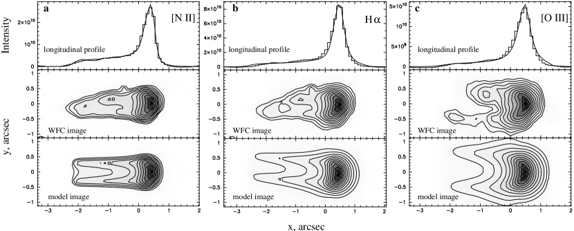
In order to restrict the range of models that we try to fit to the emission line spectra, we have used HST images of the proplyds to fix as many model parameters as possible. As an example, Figure 6 compares Wide Field Camera (WFC) images of 177–341 with simulated model images in three different emission lines. H $\alpha$ images of the heads of the proplyds allow one to determine with reasonable certainty both the radius, $r_{0}$ , of the forward-facing IF and the peak density, $n_{0}$ , in the ionized photoevaporated flow. (Estimation of this density requires that the observed surface brightness be corrected for foreground extinction.) These parameters could be estimated for all four objects and are listed in Table 1, together with the foreground extinction to each proplyd. One can also estimate the inclination angle, $i$ , of the proplyd axis to the line of sight (Henney & Arthur 1998), but this is rather uncertain and one cannot distinguish between a proplyd pointing towards or away from the observer. Additionally, estimation of $i$ was impossible in 244–440 (because of the probable influence of two ionizing stars) and in 170–337 (because of the microjet).

The relative brightness in H $\alpha$ of the proplyd tail with respect to the head allows one to determine the ratio of diffuse to direct ionizing flux, $\beta$ , although this is somewhat dependent on the assumed value of $i$ . Similarly, one can measure the quantity $l_{0}\sin i$ , where $l_{0}$ is the length of the proplyd tail. Note that the model line profiles shown in the next section are insensitive to the assumed values of $\beta$ and $\l_{0}$ , especially the latter. This is because the emission from the brightness peak of the proplyd, where the contribution from the tail is small, has been isolated in the extracted proplyd line profiles. By fitting to the [N II] and [O III] images, one can then estimate the radius, $r_{1}$ and thickness, $\Delta r_{1}$ , of the He ionization front (assumed to coincide with the ${\rm N}^{+}/{\rm N}^{++}$ and ${\rm O}^{+}/{\rm O}^{++}$ boundaries).

Table 1Proplyd parameters derived from HST images and Keck spectra

Proplyd	$\tau_{\rm f}(\mbox{H}\alpha)\,\tablenotemark{a}$	( $10^{15}\mbox{cm}$ )	( $10^{6}\mbox{cm}^{-3}$ )	(degrees)	$\beta\,\tablenotemark{e}$	$r_{1}/r_{0}\tablenotemark{f}$	$\Delta r_{1}/r_{0}\tablenotemark{f}$	(degrees)	( km s^-1)	( $10^{-7}\mbox{M}_{\odot}\,\mbox{yr}^{-1}$ )
		HST						Keck
		$r_{0}\tablenotemark{b}$	$n_{0}\tablenotemark{c}$	$i\,\tablenotemark{d}$				$i\,\tablenotemark{d,h}$	$u_{0}\tablenotemark{g,h}$	$\dot{M}\tablenotemark{i}$
170–337	1.43	$1.17$	$1.31$	—	—	—	—	$<90$	$\sim 13$	$8{\scriptscriptstyle+5\atop\raisebox{0.96873pt}{$\scriptscriptstyle-3$}}$
177–341	1.38	$1.91$	$0.636$	45–135	0.01	1.1	0.1	75–85	13–16	$9\pm 4$
182–413	1.09	$3.69$	$0.153$	0–30, 150–180	—	—	—	$>90$	$\sim 13$	$7\pm 5$
244–440	0.51	$10.4$	$0.0785$	—	—	1.25	0.2	$<90$	$\sim 13$	$15\pm 7$

^g^gfootnotetext: Initial velocity of newly-ionized gas leaving IF.^h^hfootnotetext: For 177–341, these parameters are determined from the detailed model fits to the emission line profiles (Section 7). For the other objects, they are estimated from the behaviour of the mean velocity and velocity width (Fig. 4).

For 177–341 it can be seen (Figure 6) that the models are very successful in reproducing the HST images in the three lines, especially the head of the proplyd. Although the reduced $\chi^{2}$ of the fits is typically in the range 5–20, this is mainly because of the small but significant deviations from cylindrical symmetry of the proplyd, which obviously cannot be captured in the current models. The quality of the fit near the tips of the cusp is much improved with respect to the models presented in Henney & Arthur (1998), which did not include the effect of the diffuse ionizing radiation. Although the fits to the tail well reproduce the intensity profile along the proplyd axis (top panels of Figure 6), the model images have tails that are significantly wider than observed, indicating that the tails are not the cylinders assumed in the model, but instead taper towards their tip. The ionization stratification in the proplyd is readily apparent from the increase in size of the images as one passes from [N II] through H $\alpha$ to [O III]. The best-fit models have $r_{1}/r_{0}=1.1$ , so that radius of the ${\rm N}^{+}/{\rm N}^{++}$ and ${\rm O}^{+}/{\rm O}^{++}$ transition (presumably corresponding to the He ionization front) is about 10% larger than the radius of the H ionization front. One also needs quite a broad ${\rm N}^{+}/{\rm N}^{++}$ transition ( $\Delta r_{1}/r_{0}=0.1$ ) in order to reproduce the intensity profile of the [N II] image.

For the other three proplyds, although the model fits to the heads of the proplyds are satisfactory in all cases, the fits to the tails are much less convincing than in the case of 177–341. This is mainly because the assumption of a cylindrical tail is an even poorer approximation for these objects, which all show tails that are more conical in form. Additionally, 182–413 and 244–440 both show substantial deviations from cylindrical symmetry with respect to the direction of the ionizing star. In the case of 244–440, this is probably because the proplyd is influenced both by $\theta^{1}\,$ C Ori and $\theta^{2}\,$ A Ori. The same may be true of 182–413, although in this object it is only the tail which shows the asymmetry. Alternatively, the tail in this object may be influenced by the orientation of the circumstellar disk, either via an anisotropic flow from the disk or via magnetic field lines (Bertoldi & Johnstone 1998). As a result, the parameter $\beta$ can only be reliably determined for 177–341. However, the deficiencies of the photoevaporating flow models in explaining the tails of these objects should not greatly affect the predicted line profiles for the reasons advanced earlier in this section. The position and thickness of the He ionization front could only be determined for 177–341 and 244-440 since in 182–413 the [O III] shell is too irregular to reliably determine its radius of curvature, while in 170–337 the presence of a microjet complicates the interpretation of the images.

6.1. Validation of densities derived from model fits

To obtain the peak densities, $n_{0}$ , listed in Table 1, the extinction-corrected H $\alpha$ intensities are converted into emission measures assuming that the H $\alpha$ emission coefficient is known. The ionized density at the IF on the proplyd axis is then found using the density profile predicted by the photoevaporating flow model. Although this approach seems to be robust, it is worthwhile to try and validate the densities so obtained by an independent method.

Unfortunately, the ionized densities in the proplyd flows are so large ( $10^{5}$ – $10^{6}\,\mbox{cm}^{-3}$ ) that the [S II] 6716Å/6731Å doublet ratio, which is traditionally used as a density diagnostic in ionized regions, will be in the high-density limit. Hence, it is necessary to find a diagnostic pair of lines with a higher critical density. Just such a pair exist in the ion C⁺⁺: the magnetic quadrupole transition [C III] 1907Å and the “semi-forbidden” electric dipole transition C III] 1909Å (Osterbrock 1989, p. 136). Although these lines were observed in two proplyds with the Faint Object Spectrograph (FOS) of the HST (Bally et al. 1998a), the FOS spectral resolution ( $R=1300$ ) is not sufficient to fully resolve the doublet. We are therefore grateful to Robert Rubin for allowing us access to unpublished FUV longslit spectra of the Orion nebula obtained with the Space Telescope Imaging Spectrograph (STIS), which include emission from the proplyd 159–350 (HST 3).

After subtracting the nebular contribution to the emission, we determine a value of 0.4 for the ratio [C III] 1907Å/C III] 1909Å, which corresponds to an electron density of $1.01\pm 0.05\times 10^{5}\,\mbox{cm}^{-3}$ for temperatures in the range $8000$ – $10000\,\mbox{K}$ . Henney & Arthur (1998) determined a peak density of $n_{0}=6.5\times 10^{5}\,\mbox{cm}^{-3}$ for the same proplyd. However, in order to meaningfully compare these values, two factors must be taken into account: first, that C⁺⁺ will only be present in the regions of the flow where helium is ionized, and, second, that the STIS observations sample an extended region of the proplyd containing a range of ionized densities. Both these effects should tend to make the observed C⁺⁺ density less than $n_{0}$ .

In order to quantitatively assess these effects, we employed model fits to the HST PC images of 159-350 in H $\alpha$ and [O III] 4959Å in order to determine the radius of the C⁺⁺/C⁺ transition in terms of the IF radius, $r_{0}$ (assuming that the ionization of carbon follows that of oxygen). Unfortunately, the analysis is complicated by the fact that 159–350 is a binary system (projected separation 0.5″) in which both components are proplyds. The smaller and fainter of the two proplyds, which lies between the larger proplyd and $\theta^{1}\,$ C Ori, seems to shadow part of the IF of the larger and brighter one, leading to a marked asymmetry in the appearance of the latter, especially in [O III]. As a result, we can only constrain the radius of the C⁺⁺/C⁺ transition to lie in the range 1.2–1.4 $r_{0}$ . Using these values, we than calculate from our models the emissivity-weighted mean density in the C⁺⁺ zone in an aperture corresponding to the STIS observations. For a peak density of $n_{0}=6.5\times 10^{5}\,\mbox{cm}^{-3}$ , this density turns out to be $0.9$ – $1.1\times 10^{5}\,\mbox{cm}^{-3}$ , in excellent agreement with the observed value given above.

The concordance we find in this object between the densities derived from our model fits and those obtained from the C⁺⁺ doublet give us confidence that the model-derived densities are indeed accurate.

7. Model fits to the proplyd line profiles

Although the methods discussed in the previous section allow one to fix many of the model parameters by comparison with HST images of the proplyds, there are some parameters which are not very well constrained in this way. Of these, the inclination, $i$ , and the initial Mach number, $M_{0}$ , of the photoevaporating flow are the parameters that have most effect on the predicted model line profiles. Hence, by comparison of model predictions with the observed line profiles one can both check the validity of the photoevaporating flow model and try to determine these two parameters. In this section, we concentrate on the proplyd 177–341, both because the data quality of the observed line profiles are highest in this object and because the HST images show a high degree of consistency with the simple photoevaporating flow models employed. The data quality is also high for 244–440, but in this case the interpretation is complicated by the probable influence of two ionizing stars. This object, which is also the only object to be clearly resolved spatially at ground-based resolutions, will be discussed further in a subsequent paper. For the remaining two proplyds, 170–337 and 182–413, the quality of the extracted spectra is too low to meaningfully derive parameters from the model fits.

Figure 7 shows the results of fitting such models to the observed line profiles. The fitting procedure is to perform a $\chi^{2}$ minimization of the model spectrum for various values of $i$ and $M_{0}$ , in order to determine the best-fit values of the profile normalization and velocity zero point (corresponding to the heliocentric velocity of the proplyd central star). At each step, the model is convolved with the instrumental profile and seeing before extracting a spectrum from an aperture identical to that used in the observations. Results are shown in the figure for models with $M_{0}=1$ . For each emission line, the figure shows the fit for the value of $i$ that gives the lowest value of $\chi^{2}$ , plus the highest and lowest values of $i$ that give an acceptable fit (taken as $\chi^{2}/\nu<3$ , where $\nu$ is the number of degrees of freedom). Also shown in the figure is the best-fit static model, in which the line broadening is due solely to the thermal Doppler effect (together with fine-structure splitting in the case of He I 5676Å).

It can be seen that the models fit quite well and that the inclination of this object is well constrained to lie in the range $i=75$ – $85^{\circ}$ , consistently between the different emission lines. The derived velocity zero point ( $\simeq 22$ km s^-1) is also similar for all the lines and is consistent with the centroid velocity of the [O I] 6300Å emission. The static model completely fails to fit the observed line profiles. Similarly acceptable fits are found for all $M_{0}<1.2$ .

The mass loss rate of the photoevaporating flow in the best-fit model is $9.4\times 10^{-7}\mbox{M}_{\odot}\,\mbox{yr}^{-1}$ , with the contributions of the flows from the head and the tail being roughly equal. This derived mass loss rate is directly proportional to $u_{0}n_{0}r_{0}^{2}$ , where $u_{0}=13M_{0}$ km s^-1 is the initial velocity of the photoevaporating flow, $n_{0}$ is its peak density, and $r_{0}$ is the radius of the ionization front (Table 1), each of which are known to an accuracy of 10–20% (Henney & Arthur 1998). Additionally, the parameters of the proplyd tail, which provides half the mass loss, are less well constrained by the fits than those of the head. As a result, we estimate that the uncertainty in the derived mass loss rate is of order 50%.

8. Discussion

In this section, we critically discuss the mass loss rates determined by us and by previous authors, together with the observational measurements of the disk masses and the implications of these for the length of time that the proplyds have been exposed to ionizing radiation.

8.1. Derived mass loss rates

We have performed high spectral resolution spectroscopy of four proplyds in several different emission lines. We have shown that the proplyd line width increases with ionization potential, which is consistent with the idea that the ionized gas in the proplyds comprises an accelerating ionization-stratified flow. Detailed model fitting to 177–341, which is the proplyd with the highest quality data, shows that the ionization front in this object is approximately D-critical and gives a mass loss rate in the evaporated flow of $9\pm 4\times 10^{-7}\mbox{M}_{\odot}\,\mbox{yr}^{-1}$ . Static models were found to be completely unable to fit the observations

The other proplyds all show similar linewidths to 177–341 (Figure 4), implying that the flow speeds in these objects are also similar, even in the absence of detailed model fits to the line profiles. That being the case, one can use the parameters deduced from model fits to the HST images (Section 6) to calculate the mass loss rates of these objects by scaling the value for 177–341. The resultant rates are $\dot{M}=8\times 10^{-7}$ , $7\times 10^{-7}$ , and $1.5\times 10^{-6}\mbox{M}_{\odot}\,\mbox{yr}^{-1}$ for 170–337, 182–413, 244–440, respectively.⁵⁵5For 244–440, the value obtained by scaling the result for 177–341 has been divided by two because of the lack of a prominent tail in this object. Assuming that the flow speeds are the same in all proplyds, not just those observed in the present study, then one can calculate $\dot{M}$ for all proplyds that have well-determined values of $r_{0}$ and $n_{0}$ . Taking the sample from Henney & Arthur (1998), which comprises 29 proplyds within 30 arcsec of $\theta^{1}\,$ C Ori, one then finds the distribution of mass loss rates shown in Figure 8. It can be seen that the four proplyds in the current sample have higher than average mass loss rates and indeed the mean value for the combined samples is only $\dot{M}=4.1\times 10^{-7}\mbox{M}_{\odot}\,\mbox{yr}^{-1}$ .

8.1.1 Comparison with previous mass loss determinations

The mass loss rates that we derive can be compared with previous estimates, starting with those of Churchwell et al. (1987). These authors used a method similar to ours, except that they used interferometric images of the 2 cm radio free-free emission in order to estimate the emission measure of the ionized gas. Furthermore, they had to assume that the gas was expanding at the sound speed (an assumption that is confirmed by the present work) and they employed a simplified, spherically symmetric model of the ionized photoevaporating flow. They found mass loss rates between $2\times 10^{-7}$ and $10^{-6}\mbox{M}_{\odot}\,\mbox{yr}^{-1}$ for 6 of the proplyds closest to $\theta^{1}\,$ C Ori. These estimates agree closely with our own derived mass loss rates from the same objects, which is not surprising given the similarity in methodologies.

An independent way of estimating the proplyd mass loss rates was first employed by Johnstone et al. (1998) and subsequently refined by Störzer & Hollenbach (1999). This method supposes that the mass loss is controlled by the FUV photons incident on the circumstellar disk, which heat the disk surface and drive a photodissociated neutral photoevaporating flow. This flow will autoregulate so that the FUV flux that penetrates to the base of the flow is just sufficient to heat the gas at the disk surface to a temperature such that its sound speed exceeds the local escape velocity. The mass loss rate is then directly proportional to the disk radius multiplied by the velocity multiplied by the column density of the neutral flow. Störzer & Hollenbach (1999) calculate this column density using both equilibrium and non-equilibrium PDR codes and find only a shallow dependence on the distance of the proplyd from $\theta^{1}\,$ C Ori. They then use this result to determine the mass loss rates for a sample of 10 proplyds for which the disk radius has been estimated or measured. Two of the 4 objects in our spectroscopic sample (182–413 and 171–340) are also modelled by them and for these objects they determine mass loss rates that are slightly less than half the rate determined by us. However, Störzer & Hollenbach only consider the mass loss from the directly illuminated face of the disk, whereas the diffuse nebular FUV radiation should also cause mass loss from the back face of the disk. In fact, as pointed out by Johnstone et al. (1998), since the mass loss rate is only a weak function of the FUV flux, the mass loss from the back face should be nearly as large as that from the front.⁶⁶6This is compatible with our finding that at least half the proplyd mass loss occurs through the tails in some objects, although it should be pointed out that material leaving the directly illuminated face of the disk may end up in the tail, either because the disk axis is not aligned with the proplyd axis, or through lateral pressure gradients in the shocked neutral layer between the disk and the IF. Hence, taking into account the flow from both faces would bring Störzer & Hollenbach’s mass loss rates into reasonable agreement with our own, especially considering that the velocity of the neutral flow is not very well constrained in their models.

O’Dell (1998) suggested that a confining force acted on the proplyd “atmospheres”, resulting in very low mass loss rates. However, our spectroscopic results conclusively rule out this possibility. Although only one of our proplyds was suitable for fitting to detailed models, all of them showed excess line broadening. If this broadening is due to free expansion, as seems likely, then this means that all of the objects studied are undergoing significant mass loss. The exponential decay in the density of the proplyd atmospheres found by O’Dell (1998) can equally well be explained by the freely expanding models we have calculated here and the large line widths are a direct indication that the static model does not apply. This means that it is not necessary to seek the operation of a confining force (O’Dell 1998), which is just as well, for we now understand that the only force sufficiently strong to confine the atmospheres (Ly $\alpha$ radiation pressure) was incorrectly derived, with the magnitude estimated by O’Dell (1998) being, at best, an upper limit (Henney & Arthur 1998). Therefore, one must look to other novel methods for explaining the existence of circumstellar envelopes in such an intense photoionizing radiation field.

The one caveat to our conclusion arises from our assumption that the mechanism producing the non-thermal, non-Kolmogorov line broadening in the main body of the nebula is not operating in the ionized atmosphere of the proplyds. This line broadening is about 10 km s^-1 (O’Dell 1994, 1999) and is common to all lines and ions. One explanation of the extra broadening is that of Ferland (1999) who proposes that it is due to Alfvén waves, a mechanism thought to explain the non-thermal line broadening in molecular clouds. The ad hoc addition of such an additional broadening of the lines would possibly reduce the mass loss rates necessary to explain the observed broad profiles of the proplyd spectra; but, without understanding the process in the nebula, we cannot introduce it into our proplyd models. If the Alfvén wave broadening in 177-341 were the same as that proposed in the main body of the nebula, then the derived mass loss rate would hardly be reduced. Invoking larger values for any Alfvén wave component seems without justification without understanding the physics of this process. Besides, an extra broadening component of even 10 km s^-1 would pose problems for the model fits to the [N II] 6583Å line, whose width is currently well reproduced by the broadening due to the expansion of the ionized gas alone. It is possible that the extra broadening seen in the nebula is due to the kinematics of the gas, rather than to Alfvén waves (e.g. Yorke, Tenorio-Tagle & Bodenheimer 1984), although it must be conceded that such a “kinematic” broadening mechanism seems incapable of explaining the observed width of the [O I] line.

8.2. Implications for proplyd evaporation times

Now that we have reliable estimates for the proplyd mass loss rates, we are in a position to calculate their evaporation times if we can only estimate the mass of the circumstellar disks contained within them. Discounting the mass of the star itself, the disks should dominate the mass of the proplyd. The calculated masses of the combined neutral and ionized envelopes are only of order $10^{-5}M_{\odot}$ , which would imply evaporation times, $t_{\rm e}\equiv M/\dot{M}$ , as short as 10–100 years unless a substantial reservoir of gas in the form of an accretion disk were present. We now know from both observations and theory that most of the mass resides in an inner disk, which means that the depletion of that mass will determine the survival of the proplyds. In this section we summarise the arguments leading to estimates of the disk masses and discuss the problem of their predicted short lifetimes, which conflict with their ubiquity.

Johnstone et al. (1998) show that for a disk whose surface density follows a power law in radius, then $t_{\rm e}$ calculated using the current values of the disk mass and mass loss rate should be proportional to the length of time since the disk was first exposed to FUV/EUV radiation, the constant of proportionality being unity if the mass loss is controlled by the FUV radiation and if the surface density follows the standard $r^{-3/2}$ law (Adams, Shu & Lada 1988). According to this picture the disks started with much larger sizes, masses and mass loss rates than they have today and have shrunk to their current size due to photoevaporation, with the disk mass declining in time as $t^{-1}$ and the disk radius and mass loss rate declining as $t^{-2}$ . Projecting a proplyd’s evolution into the future, $t_{\rm e}$ is hence the time it will take for the disk to lose half its current mass and shrink in radius by a factor of 4. If the disk radius was initially truncated by some other process (Hollenbach et al. 2000) before it was exposed to UV radiation, then $t_{\rm e}$ would only be an upper limit to the exposure time.

8.2.1 Disk masses

The masses of the circumstellar disks associated with the Orion proplyds have been estimated by two different methods. The first involves measuring the extinction by the silhouette disks of the background nebular emission and gives only lower limits on the disk mass (O’Dell & Wen 1994; McCaughrean & O’Dell 1996; McCaughrean et al. 1998; Throop et al. 1998). Assuming “standard” dust properties, the values found are typically $10^{-6}$ – $10^{-4}M_{\odot}$ . Throop et al. (1998), on the other hand, suggest that substantial dust coagulation has ocurred in the disks, resulting in grains larger than 10 $\mu$ m, which would imply that these lower limits should be revised upward by several orders of magnitude. However, this result is based on a claimed wavelength independence of the size of the silhouette disks, which seems inconsistent with the finding of McCaughrean et al. (1998) that the silhouette of the giant disk 114–426 appears 20% smaller in Pa $\alpha$ (1.87 $\mu$ m) than in H $\alpha$ (0.66 $\mu$ m).

The second method is to search for mm-wavelength thermal emission from dust in the disks. The first attempt to do this was by Mundy et al. (1995), who observed a 45″ radius region of the central Trapezium Cluster at 3.5 mm with an angular resolution of approximately 1″. Although they detected emission from several proplyds (notably, 167–317, 158–323, 168–326 and 159–350), in no case was the 3.5 mm flux larger than the 2 cm flux measured by Felli et al. (1993). This implies that the 3.5 mm emission is dominated by free-free radiation in the ionized gas or non-thermal processes, rather than by the thermal emission of dust in the accretion disk. Hence, only upper limits on the disk masses could be determined. These were $<0.15M_{\odot}$ for individual sources and $<0.03M_{\odot}$ for the average mass of all disks in their surveyed region. Subsequently, Lada et al. (1996), using higher sensitivity observations at 1.3 mm, reported the detection of thermal dust emision from 3 proplyds (roughly one quarter of those present in their fields) with deduced disk masses lying between $0.007$ and $0.016M_{\odot}$ . More recently Bally et al.(1998b) has detected thermal emission, also at 1.3 mm, from the giant silhouette disk 114–426, which implies a mass for this object of $0.02M_{\odot}$ , together with an upper limit for the disk mass of 182–413 (one of our spectroscopic sample) of $<0.015M_{\odot}$ . These authors also derive independent upper limits to the disk masses in these two systems from the lack of observed ¹³CO emission, but these latter estimates depend critically on the CO abundance in the disks, which is very uncertain (Dutrey et al. 1996).

In summary, if the results of the mm continuum studies are taken at face value, then the disk masses range from $0.02M_{\odot}$ in the largest silhouette disk (disk radius $\simeq 1\arcsec$ ) through $\simeq 0.01M_{\odot}$ for the largest of the bright proplyds (disk radii $\simeq 0.1\arcsec$ ) down to upper limits of $<0.005M_{\odot}$ for the majority of proplyds (disk radii $<0.05\arcsec$ – $0.1\arcsec$ ). These can be compared with the masses measured by the same technique for disks around classical T Tauri stars of similar ages to those in the Trapezium cluster, but located in isolated star forming regions such as Taurus, Ophiuchus and Lupus, which are in the range $10^{-4}$ – $10^{-1}M_{\odot}$ (Osterloh & Beckwith 1995; Dutrey et al. 1996; Nürnberger et al. 1997a,b). Taking that subsample of the disks observed by Osterloh & Beckwith (1995) whose central stars have estimated ages between $10^{5}$ and $10^{6}$ years ( $N=18$ ), one finds a mean mass of $0.017M_{\odot}$ , although Hartmann et al. (1998) suggest that the Osterloh & Beckwith masses may be underestimated by a factor of 2.5.

Hence, there is no obvious conflict between the low masses found for the disks around the stars in the dense Trapezium Cluster and those found in more quiescent regions of low-mass star formation: the largest disks in Orion have a mass typical of those around T Tauri stars, whereas the disks inside the bright proplyds have lower masses because of the photoevaporation-induced mass loss. However, the masses derived for the disks in Orion are extremely uncertain because of their sensitivity to the disk temperature and the mm-wavelength opacity of the dust. Many isolated T Tauri disks have well-measured spectral energy distributions from infrared to mm wavelengths, allowing reasonable confidence in the fitting of multi-parameter disk models. For the Orion disks, on the other hand, the disk masses are estimated from measurements at a single wavelength and are hence much less reliable. More importantly, the magnitude and wavelength dependence of the dust opacity is very poorly known, as is the dust-gas ratio in the disks (Beckwith 1999). In addition, the mass estimates assume that the disks are optically thin, whereas at 1.3 mm the disks should become optically thick for radii within $\simeq 10\mbox{AU}$ of the central star (Hartmann et al. 1998), which is comparable to the outer radii of the smaller proplyd disks.⁷⁷7For edge-on disks, such as in 182–413, optical depth effects will become important at even larger radii.

If the disk masses derived from mm continuum observations are correct, then the evaporation times would be $t_{\rm e}\simeq 10^{4}$ years for the larger proplyds ( $M\simeq 0.01M_{\odot}$ , $\dot{M}\simeq 10^{-6}\mbox{M}_{\odot}\,\mbox{yr}^{-1}$ ) and $t_{\rm e}\leq 2.5\times 10^{4}$ years for the smaller ones ( $M\leq 0.005M_{\odot}$ , $\dot{M}\simeq 2\times 10^{-7}\mbox{M}_{\odot}\,\mbox{yr}^{-1}$ ). However, as a result of the uncertainties discussed in the previous paragraph, the quoted disk masses and hence the estimated evaporation times can probably not be trusted to better than an order of magnitude.

8.2.2 The age of the Orion nebula

The ages of the low- to intermediate-mass stars in the Orion Nebula Cluster range from roughly $10^{4}\mbox{--}10^{7}$ years, as determined by fitting evolutionary tracks to the observed color-luminosity diagram (Hillenbrand 1997). Taking that subsample ( $N=58$ ) of the stars in Hillenbrand (1997) that both have measured ages and are listed as proplyds in O’Dell & Wong (1996), one finds that the mean and standard deviation of the logarithm of the stellar ages is $\log(t)=5.45\pm 0.95$ .⁸⁸8It should be noted that these ages are somewhat sensitive to which stellar evolution calculations are used. The quoted values employ the calculations of D’Antona & Mazitelli (1994), whereas the calculations of Swenson, et al. (1994) give ages that are typically 2–3 times larger. The ages of the high-mass stars, such as $\theta^{1}\,$ C Ori, are much harder to determine observationally but, in the absence of evidence to the contrary, are likely to lie in the same range.

The derived photoevaporation times are thus small compared with the stellar ages, even taking into account possible errors in the disk mass estimates. Hence, one must look for other mechanisms that may have saved the proplyd disks from exposure to UV radiation until relatively recently. One possibility, independently suggested by Bally et al. (1998b) and Henney & Arthur (1998), is that the ionized zone around $\theta^{1}\,$ C Ori was maintained in an ultracompact stage (e.g. Kurtz, et al. 2000 and references therein) for much of the lifetime of the ionizing star and has only recently undergone an “inflationary phase”, in which it expanded to its current size. The problem with this argument is that the Orion nebula has a diameter of approximately 3 parsecs ( $10^{19}\mbox{cm}$ ), as revealed by long-exposure optical photographs. Hence, if it were to have been much smaller $10^{4}$ years ago, its expansion velocity must be of order $150\mbox{$\,$km s${}^{-1}$}$ . This is more than ten times the sound speed in the ionized gas and seems implausibly high, even for an H II region in the champagne phase (e.g. Yorke 1986). Numerical hydrodynamic simulations (Yorke et al. 1984; García-Segura & Franco 1996) show that the ionized gas can only reach velocities of order $40\mbox{$\,$km s${}^{-1}$}$ , or $80\mbox{$\,$km s${}^{-1}$}$ if one includes the effect of the stellar wind from the ionizing star (Comerón 1997). On the other hand, the expansion of the IF need not necessarily involve physical movement of the gas: if the motion of $\theta^{1}\,$ C Ori had recently caused it to emerge from the background molecular cloud, then an R-type IF may have rapidly propagated out to the observed size of the nebula. However, the shell-like appearance of the outer boundary of the nebula would argue against this idea. Besides, in order for $\theta^{1}\,$ C Ori to have travelled the $\simeq 3\mbox{--}6\times 10^{17}\mbox{cm}$ from the background cloud to its present position (Baldwin et al.1991; Wen & O’Dell 1995) in the last $10^{4}$ years, its velocity must be of order $10\mbox{--}20\mbox{$\,$km s${}^{-1}$}$ , which is much higher than the velocity dispersion of the stars in the cluster.⁹⁹9Note, however, that just such a high blue shift of $\theta^{1}\,$ C Ori is implied by the study of Stahl et al. (1996), but the history of spectral variations and large range of derived radial velocities (O’Dell 1999) make it most likely that one is seeing peculiar atmospheric effects rather than the systemic velocity of the star. The fact that the principal emitting layer in the core of the nebula has an effective thickness less than the distance of $\theta^{1}\,$ C Ori from the IF (Wen & O’Dell 1995) is also more consistent with a highly evolved champagne region than one in which the “blowout” occurred recently (G. García-Segura, priv. comm.). It is possible, however, that other, less massive stars in the region are partly responsible for ionizing the nebula on large scales (e.g. $\iota\,$ Ori, O’Dell et al. 1993a) and these may be at a sufficient distance from the proplyds that they have induced little disk evaporation themselves.

A further argument against the recent expansion of the H II region is the statistical unlikelihood of catching $\theta^{1}\,$ C Ori during such a short-lived phase of its evolution. This statistical argument also weighs against the related proposal (Bally et al. 1998b) that $\theta^{1}\,$ C Ori has only recently reached the main sequence and begun emitting ionizing photons. A similar argument would seem to rule out the suggestion (S. Lizano, priv. comm.) that massive circumstellar envelopes have protected the disks from evaporation until recently, given that none of the bright proplyds show any surviving trace of such an envelope.¹⁰¹⁰10Although one of the bright proplyds, 244–440, is very much larger than the others, the visibility of the central star implies that any extended envelope in this object cannot be more massive than about $10^{-4}M_{\odot}$ .

8.2.3 Kinematics of the proplyd stars

Since the stars move inside the potential well of the cluster, it may be that the stellar motions themselves are the limiting factor in determining the exposure time to evaporation of the proplyd disks. Jones & Walker (1988) calculated the proper motions of hundreds of ONC stars and found a one-dimensional velocity dispersion of $\sim 2.5\mbox{$\,$km s${}^{-1}$}$ , which hardly varies with radius in the cluster. Such an “isothermal” behaviour of the velocity dispersion is consistent with the derived stellar density distribution (Henney & Arthur 1998), which is close to $r^{-2}$ outside of a core radius of $10\mbox{--}15\arcsec$ around $\theta^{1}\,$ C Ori, which lies very close to the center of the cluster. Additionally, Jones & Walker show that the stellar velocities are closely isotropic in all but the outermost regions of the ONC, which means that the above velocity dispersion should also be a typical velocity along the radius joining the star to the cluster center.

The effect of stellar motions on the proplyd exposure time was first explored in detail by Störzer & Hollenbach (1999) who noted that beyond a critical distance, $r_{\rm cr}$ , from $\theta^{1}\,$ C Ori, the FUV flux is too weak to heat the disk surface sufficiently for it to escape from the gravitational potential of the central star (Johnstone et al. 1998). In such a case, the disk evaporation is controlled by the ionizing EUV flux and the mass loss rate falls with distance as $r^{-1}$ . Störzer & Hollenbach argue that a proplyd on an eccentric orbit that moves from larger to smaller radii in the cluster is likely to have an evaporation time, $t_{\rm e}$ , roughly equal to its dynamic time, $t_{\rm d}\equiv r/u$ , during most of its evolution outside of $r_{\rm cr}$ . Inside $r_{\rm cr}$ the mass loss is controlled by the FUV flux and is hence only weakly dependent on distance. They claim that this leads to a “freezing” of the proplyd for $r<r_{\rm cr}$ since $t_{\rm d}$ becomes smaller than $t_{\rm e}$ , resulting in the proplyd disk mantaining a roughly constant size during its crossing of the cluster core. They calculate a value $r_{\rm cr}\simeq 0.2$ parsec in Orion (implying a duration of $\simeq 8\times 10^{4}$ years for the passage from $r_{\rm cr}$ to the cluster center) and proceed to estimate the disk masses for a sample of 10 proplyds for which they have determined model mass loss rates (see Section 8.1.1 above), obtaining values in the range $0.002\mbox{--}0.01M_{\odot}$ . Such a procedure is the converse of the approach adopted here, in which we proceed from the mass loss rates and the mm-continuum disk masses in order to estimate the exposure time to ionizing radiation.

The disk masses obtained by Störzer & Hollenbach (1999) for their sample seem to be consistent with the estimates from mm-continuum observations (Section 8.2.1). However, there are two problems with their analysis, which may result in their mass loss rate being underestimated by a factor of about 8. Firstly, rather than use the current mass loss rate in their calculations, they use the mass loss rate that the proplyd would have when placed at a distance $r_{\rm cr}$ , but using the current value for the disk radius. This ignores the fact that most of the proplyds in their sample are at $r\ll r_{\rm cr}$ so that, even though $t_{\rm e}>t_{\rm d}$ inside of $r_{\rm cr}$ , these proplyds will have lost half their mass and shrunk in radius by a factor of 4 since they were at $r_{\rm cr}$ . Secondly, their mass loss rates are generally smaller than the rates that we determine for the same proplyds by a factor of at least 2. As discussed in Section 8.1.1, this is probably mainly due to their neglect of the flow from the back side of the disk. Taking these two factors into account results in disk masses that are now in conflict with those estimated from mm-continuum observations. This is consistent with the fact that the $\simeq 8\times 10^{4}$ year crossing time for the cluster core is large compared to the $\simeq 2\times 10^{4}$ year disk evaporation time calculated in Section 8.2.1.

It is notable that for all proplyds in our spectroscopic sample except 170–337 the proplyd [O I] 6300Å line is significantly blueshifted by 3–7 km s^-1 with respect to the nebula (Figure 4). The nebular [O I] 6300Å emission (Wen & O’Dell 1992) is believed to originate from the PDR behind the IF on the surface of the background molecular cloud OMC–1 and is typically blueshifted by 1–2 km s^-1 with respect to the CO emission (Sugitani et al. 1986; O’Dell et al. 1993a). If the [O I] emission from the proplyds traces the velocity of the enclosed low-mass star, then this implies that 3 of the 4 proplyd stars in our sample are moving away from the molecular cloud at 5–9 km s^-1. These velocities are rather large compared with the velocity dispersion implied by proper motion studies (see above). Re-analysis of published proper motion data (Jones & Walker 1988) for a sample of proplyds ( $N=21$ ) and a sample of non-proplyd stars ( $N=35$ ) lying within the core of the nebula shows no significant difference between the velocity dispersion of the two samples ( $2.8\pm 0.5$ km s^-1 for the proplyds; $2.7\pm 0.3$ km s^-1 for the non-proplyds). Although many proplyds do have quoted proper motions larger than this, they also have large estimated uncertainties in the proper motion (following Jones & Walker, only stars with uncertainties $<0.1\arcsec/\mbox{century}$ are included in our two samples). It seems likely then that 3 of our 4 proplyds are very atypical in their high velocities away from the background molecular cloud. This need not be surprising since these 3 objects are among the largest proplyds and hence may have only recently been exposed to ionizing radiation. One would therefore expect these proplyds to either lie close to the background IF or to have high blue-shifted velocities (away from the molecular cloud), or both.

Such an interpretation of the [O I] velocity shift in terms of the stellar motion depends on there being no systematic asymmetry in the line profile due to the kinematics of the neutral outflow. Such an asymmetry could arise, for instance, if the [O I] emission came predominantly from the base of the neutral flow. In this case, the receding portion of the flow would be occulted by the opaque disk, leading to a systematic blueshift in the line with respect to the stellar velocity. However, the observations of Bally et al. (1998) show that the majority of the [O I] 6300Å emission comes from the IF and that region of the PDR just behind it, rather than from material near the disk. In this case, the upper limits established in sections 4.1 and 7 on the optical depth through the neutral envelope imply that the extinction-induced asymmetry in the line should be small, which is consistent with the appearance of the [O I] 6300Å line. Although this line does show a slightly enhanced blue wing, the difference between the mean velocity and the peak velocity of the line is in all cases less than 2 km s^-1. If the peak [O I] velocity were a truer tracer of the stellar velocity than the mean [O I] velocity, then this would reduce the blueshifts of the stars with respect to the molecular cloud to an average of $5\mbox{$\,$km s${}^{-1}$}$ for the 3 high-velocity proplyds, leading to an exposure time of approximately $6000(z/10^{17}\mbox{cm})$ years, where $z$ is the current distance of the proplyd from the background IF. This could be reconciled with the exposure time estimated in Section 8.2.1 if $z\leq 2\times 10^{17}\mbox{cm}$ , which would place all 3 proplyds behind $\theta^{1}\,$ C Ori, which lies at $z\simeq 3\mbox{--}6\times 10^{17}\mbox{cm}$ . The inclination angle of $75^{\circ}$ determined for 177–341 (Section 7) is consistent with this if the distance between $\theta^{1}\,$ C Ori and the background IF is at the low end of the estimated range.

8.2.4 Is there still a “lifetime problem”?

The previous two sections indicate that none of the mechanisms that have been proposed to reduce the time for which the proplyds have been exposed to ionizing radiation are capable of producing exposure times as short as the one or two times $10^{4}$ years that are demanded by our measured mass loss rates, coupled with the masses determined from mm-continuum observations. Hence the “lifetime problem” has not gone away, and the undeniable existence of the proplyds leaves one in the situation of having to reject either the mass loss rates or the measured masses. The numerical factors involved are not large: a reduction of one or the other by a factor of 5 would be sufficient to render plausible either the “young H II region” or the “moving stars” hypothesis. We maintain, however, that the uncertainty in our mass loss determinations are much less than this, depending as they do only on the size of the IF and the density and velocity of the ionized gas, which have all now been directly measured.

For well-resolved proplyds, the only significant error in the IF size is due to the assumed distance to the nebula. Since we adopt a value of 430 pc, which is at the low end of published estimates, any error here is only likely to be in the direction of our having underestimated the mass loss rate. We have determined the ionized density in two different ways. The principal method is to determine the emission measure of the proplyd cusp from the H $\alpha$ surface brightness, after correcting for foreground extinction. This has uncertainties of order 20% due to the effects of geometry and the possibility of extinction local to the ionized flow (Henney & Arthur 1998). However, since we employed the dust-free value in our calculations, we are again more likely to have underestimated rather than overestimated the mass loss rate. Furthermore, the density so-determined is consistent with an independent determination from the C⁺⁺ doublet ratio in 159–350 (Section 6.1). The velocity of the ionized flow just outside the IF is constrained to be $13\mbox{--}16\mbox{$\,$km s${}^{-1}$}$ from our spectroscopic measurements (Sections 4 and 7). Again, we use the lower value when calculating the mass loss rates. Although the outflow velocity has only been measured directly in four objects, which are atypically large, there is no reason to expect that this velocity will be any different in the smaller proplyds. It is possible that we have overestimated the mass loss rate through the proplyd tails, since the observed tails show a tapering, which is not present in the models and may result in the area of the IF in the tail being less than we have supposed. However, since the tails only amount for about half the proplyd mass loss, reducing the tail area by even a factor of 2 would only diminish the total mass loss rate by 25%.

In summary, the uncertainty in our mass loss rate determinations for individual proplyds is probably less than 50% and the rates are more likely to be underestimated than overestimated. There is no apparent potential source of error that could have led to our systematically overestimating the mass loss rates by a significant amount. We conclude, therefore, that any error must lie in the disk mass estimates. Indeed, even disregarding uncertainties in the disk temperature and the importance of optical depth effects (see Section 8.2.1), these estimates are completely dependent on the assumed value of the dust opacity at mm wavelengths. This opacity could quite easily be a factor of 5 smaller than the canonical value of $0.02\,\mbox{cm}^{2}\mbox{g}^{-1}$ (Beckwith 1999), either because of a reduced dust-gas ratio or because of the dust optical properties differing from those supposed.

8.3. Future work

Clearly, there are many unanswered questions concerning the mass loss rate and lifetime of the Orion Nebula proplyds. We can identify the following as approaches that will help resolve the situation. We need accurate emission line profiles for more proplyds than 177–341 and this expanded sample needs to include a variety of intrinsic distances from $\theta^{1}\,$ C Ori. The key to obtaining this improved sample is through more accurate subtraction of the nebular background. This can best be done using the HST and we are able to report that Cycle 8 time has been allocated for just that, but only for the object 167–317, which lies close to $\theta^{1}\,$ C Ori. It will be observed using the density sensitive doublet C III] at 1909Å. The power of the Keck I+HIRES system would also allow measurement of more proplyds from the ground. We need to determine the true radial velocity of $\theta^{1}\,$ C Ori, which is presently highly uncertain, the most recent determinations being very different from earlier values (Stahl, et al. 1996, O’Dell 1999), with both the old and new values indicating large relative motions (but in opposite directions) with respect to the molecular cloud. We also need to have a self consistent model of the main body of the nebula, i.e. one that can explain both the current structure and flow of material, which will also demand explaining the small scale line broadening that may arise from Alfvén waves. It is important, too, to pursue observations and models that can guide us in understanding the role of extinction within the proplyd material. Finally, more reliable estimates of the disk masses are vital, although obtaining these poses formidable observational and theoretical challenges.

WJH acknowledges financial support from DGAPA-UNAM project IN128698 and from CONACyT project E-25470, Mexico; CRO’s work was supported in part by NASA grant NAG5-1626 and STScI grant GO-06603.02 to Rice University. We are very grateful to Jane Arthur, Vladimir Escalante, David Hollenbach, Doug Johnstone, and Herbert Störzer for many useful suggestions and discussions. Brian Cudnik assisted in the early steps of data reduction and Francisco Valdes of NOAO prepared the special procedures for reducing the two dimensional HIRES spectra. We are indebted to the generosity of both John Stauffer of the Center for Astrophysics for his cooperation in shared night observing with the Keck and Robert Rubin for allowing us to use his unpublished STIS spectra of 159–350.

References

(1)
(2) Bally, J., Sutherland, R. S., Devine, D., & Johnstone, D. 1998a, AJ, 116, 293
(3)
(4) Bally, J., Testi, L., Sargent, A., & Carlstrom, J. 1998b, AJ, 116, 854
(5)
(6) Baldwin, J. A., Ferland, G. J., Martin, P. G., Corbin, M. R., Cota, S. A., Peterson, B. M., & Sletteback, A. 1991, ApJ, 374, 580
(7)
(8) Beckwith, S. V. W. 1999, in The Physics of Star Formation and Early Evolution II, eds. C. J. Lada & N. D. Kylafis, (CITY: PUBLISHER), in press
(9)
(10) Bertoldi, F. 1989, ApJ, 346, 735
(11)
(12) Bertoldi, F. & Johnstone, D. 1999, in ASP Conf. Ser. 12?, The Orion Complex Revisited, ed. McCaughrean, M. J. (San Francisco: ASP), in press
(13)
(14) Castañeda, H. O. 1988, ApJS, 67, 93
(15)
(16) Chen, H., Bally, J., O’Dell, C. R., McCaughrean, M. J., Thompson, R. L., Rieke, M., Schneider, G., & Young, E. T. 1998 ApJ, 492, L173
(17)
(18) Churchwell, E., Felli, M., Wood, D. O. S., & Massi, M. 1987, ApJ, 321, 516
(19)
(20) Comerón, F. 1997, A&A, 326, 1195
(21)
(22) D’Antona, F., & Mazitelli, I., 1994, ApJS, 90, 467
(23)
(24) Dutrey, A., Guilloteau, S., Duvert, G., Prato, L., Simon, M., Schuster, K., & Ménard, F. 1996 A&A, 309, 493
(25)
(26) Dyson, J. E. 1968, Ap&SS, 1, 388
(27)
(28) Esteban, C., Peimbert, M., Torres-Peimbert, S., & Escalante, V. 1998, MNRAS, 295, 401
(29)
(30) Ferland, G. J. 1999, in ASP Conf. Ser. 12?, The Orion Complex Revisited, ed. McCaughrean, M. J. (San Francisco: ASP), in press
(31)
(32) Felli, M., Churchwell, E., Wilson, T., & Taylor, G. B. 1993, A&AS, 98, 137
(33)
(34) García-Segura, G. & Franco, J. 1996, ApJ, 469, 171
(35)
(36) Garay, G., Moran, J. M., & Reid, M. J. 1987, ApJ 314, 535
(37)
(38) Hartmann, L., Calvet, N., Gullbring, E., & D’Alessio, P. 1998, ApJ, 495, 385
(39)
(40) Henney, W. J. 1998, ApJ, 503, 760
(41)
(42) Henney, W. J. 1999, in prep.
(43)
(44) Henney, W. J., & Arthur, S. J. 1997, in IAU Symposium 182, Herbig-Haro Objects and the Birth of Low Mass Stars, ed. B. Reipurth & C. Bertout (Dordrecht: Kluwer), 561
(45)
(46) Henney, W. J., & Arthur, S. J. 1998, AJ, 116, 322
(47)
(48) Henney, W. J., Meaburn, J., Raga, A. C., & Massey, R. M. 1997, A&A, 324, 656
(49)
(50) Henney, W. J., Raga, A. C., Lizano, S., & Curiel, S. 1996, ApJ, 463, 216
(51)
(52) Henney, W. J., & Watson, A. M., 1999, in prep.
(53)
(54) Hillenbrand, L. A. 1997, AJ, 113, 1733
(55)
(56) Hollenbach, D., Yorke, H. W., & Johnstone, D. 2000, in Protostars and Planets IV, eds. V. Mannings, A. Boss, & S. Russell (Tucson: UAP), in press
(57)
(58) Hu, X. 1996, PhD Thesis, Rice University, Houston, Texas
(59)
(60) Johnstone, D., Hollenbach, D., & Bally, J. 1998, ApJ, 499, 758
(61)
(62) Kurtz, S., Cesaroni, R., Churchwell, E., Hofner, P., & Walmsley, M. 2000, in Protostars and Planets IV, eds. V. Mannings & A. N. Other (Tucson: UAP), in press
(63)
(64) Lada, C. J., Dutrey, A., Guilloteau, S., Mundy, L. 1996, BAAS, 189, 5301
(65)
(66) Laques, P., & Vidal, J. L. 1979, A&A, 73, 97
(67)
(68) Liu, X.-W., Barlow, M. J., Danziger, I. J., & Storey, P. J. 1995, ApJ, 450, L59
(69)
(70) Massey, R. M. & Meaburn, J. 1995, MNRAS, 273, 615
(71)
(72) McCaughrean, M. J., Chen, H., Bally, J., Erickson, E., Thompson, R., Rieke, M., Scheider, G., Stolovy, S., & Young, E. 1998 ApJ, 492, L157
(73)
(74) McCaughrean, M. J. & O’Dell, C. R. 1996, AJ, 111, 1977
(75)
(76) McCaughrean, M. J. & Stauffer, J. 1994, AJ, 108, 1382
(77)
(78) McCullough, P. F., Fugate, R. Q., Christou, J. C., Ellerbroek, B. L., Higgens, C. H., Spinhirne, J. M., Cleis, R., & Moroney, J. F. 1995 ApJ, 438, 394
(79)
(80) Meaburn, J. 1988, MNRAS, 233, 791
(81)
(82) Meaburn, J., Massey, R. M., Raga, A. C., & Clayton, C. A. 1993, MNRAS, 260, 625
(83)
(84) Mellema, G. 1993, PhD Thesis, University of Leiden, Holland
(85)
(86) Mundy, L. G., Looney, L. W., & Lada, E. A. 1995, ApJ, 452, L137
(87)
(88) Nürnberger, D., Brandner, W., Yorke, H. W., & Zinnecker, H. 1997a, A&A, 330, 459
(89)
(90) Nürnberger, D., Chini, R., & Zinnecker, H. 1997b, A&A, 324, 1036
(91)
(92) O’Dell, C. R. 1994, Ap&SS, 216, 267
(93)
(94) O’Dell, C. R. 1998, ApJ, 115, 263
(95)
(96) O’Dell, C. R. 1999, in ASP Conf. Ser. 12?, The Orion Complex Revisited, ed. McCaughrean, M. J. (San Francisco: ASP), in press
(97)
(98) O’Dell, C. R., Hartigan, P., Bally, J., and Morse, J. A. 1997, AJ, 114, 2016
(99)
(100) O’Dell, C. R., Valk, J. H., Wen, Z., & Meyer, D. M. 1993a, ApJ, 40
(101)
(102) O’Dell, C. R., Walter, D. K., & Dufour 1992, ApJ, 399, L67
(103)
(104) O’Dell, C. R. & Wen, Z. 1992 ApJ, 387, 229
(105)
(106) O’Dell, C. R. & Wen, Z. 1994, ApJ, 436, 194
(107)
(108) O’Dell, C. R., Wen, Z., & Hu, X. 1993, ApJ, 410, 696
(109)
(110) O’Dell, C. R. & Wong, S. K. 1996, AJ, 111, 846
(111)
(112) Osterbrock, D. E. 1989, Astrophysics of Gaseous Nebulae and Active Galactic Nuclei (Mill Valley, CA: University Science Books)
(113)
(114) Osterloh, M. & Beckwith, S. V. W. 1995, ApJ, 439, 288
(115)
(116) Richling, S. & Yorke, H. W. 1998 A&A 340, 508
(117)
(118) Stahl, O. & 11 others 1996, A&A, 312, 539
(119)
(120) Stapelfeldt, K., Sahai, R., Werner, M., & Trauger, J. 1997, in ASP Conf. Ser. 119, Planets Beyond the Solar System and the Next Generation of Space Missions, ed. D. Soderblom (San Francisco: ASP), 131
(121)
(122) Stecklum, B., Henning, T., Feldt, M., Hayward, T. L., Hoare, M. G., Hofner, P., & Richter, S. 1998, AJ, 115, 767
(123)
(124) Störzer, H. & Hollenbach, D. 1998, ApJ, 502, L71
(125)
(126) Störzer, H. & Hollenbach, D. 1999, ApJ, in press
(127)
(128) Sugitani, K., Fukui, Y., Ogawa, H., & Kawabata, K. 1986, ApJ, 303, 667
(129)
(130) Swenson, F. J., Faulkner, J., Rodgers, F. J. & Iglesias, C. A. 1994, ApJ, 425, 286
(131)
(132) Throop, H. B., Bally, J., Esposito, L. W., & Mccaughrean, M. J. 1998, BAAS, 193, 118.02
(133)
(134) Wen, Z. & O’Dell, C. R. 1993, ApJ, 409, 262
(135)
(136) Weidenschilling, S. J. 1984, Icarus, 60, 553
(137)
(138) Weidenschilling, S. J. & Cuzzi, J. N. 1993, in Protostars and Planets III, eds. E. H. Levy & J. I. Lunine (Tucson: UAP), 1031
(139)
(140) Yorke, H. W. 1986, ARA&A, 24, 49
(141)
(142) Yorke, H. W., Tenorio-Tagle, G.. & Bodenheimer, P. 1984, A&A, 138, 325
(143)
(144) Zuckerman, B. 1973, ApJ, 183, 863
(145)

Refer to caption — Figure 1.— (a) Line profile parameters as a function of position along the spectrograph slit for an example spectrum: [O III] 4959Å from Ori 177–341, with slit oriented parallel to the proplyd axis. The samples used in the “large sample” method are indicated by the white boxes in the top panel, while those used in the “small sample” method are indicated by the gray strips. The parameters shown are total line intensity (top panel), flux-weighted mean line velocity (center panel), and line FWHM (bottom panel, solid line). Also shown in the bottom panel (dashed line) is the quantity 2.355 $\sigma$ , where $\sigma$ is the flux-weighted RMS velocity width of the line. This quantity is equal to the FWHM for a Gaussian line. (b) Same as (a), but with slit oriented perpendicular to the proplyd axis.