The Use of Generalized Information Dimension in Measuring Fractal Dimension of Time Series

Abstract

An algorithm for calculating generalized fractal dimension of a time series using the general information function is presented. The algorithm is based on a strings sort technique and requires $O(N\log_{2}N)$ computations. A rough estimate for the number of points needed for the fractal dimension calculation is given. The algorithm was tested on analytic example as well as well-known examples, such as, the Lorenz attractor, the Rossler attractor, the van der Pol oscillator, and the Mackey-Glass equation, and compared, successfully, with previous results published in the literature. The computation time for the algorithm suggested in this paper is much less then the computation time according to other methods.

]

I Background

In the recent decades the study of chaos theory has gathered momentum. The complexity that can be found in many physical and biological systems has been analyzed by the tools of chaos theory. Characteristic properties, such as the Lyapunov exponent, Kolmogorov entropy and the fractal dimension (FD), have been measured in experimental systems. It is fairly easy to calculate signs of chaos if the system can be represented by a set of non-linear ordinary differential equations. In many cases it is very difficult to built a mathematical model that can represent sharply the experimental system. It is essential, for this purpose, to reconstruct a new phase space based on the information that one can produce from the system. A global value that is relatively simple to compute is the FD. The FD can give an indication of the dimensionality and complexity of the system. Since actual living biological systems are not stable and the system complexity varies with time, one can distinguish between different states of the system by the FD. The FD can also determine whether a particular system is more complex than other systems. However, since biological systems are very complex, it is better to use all the information and details the system can provide. In this paper we will present an algorithm for calculating FD based on the geometrical structure of the system. The method can provide important information, in addition, on the geometrical of the system (as reconstructed from a time series).

The most common way of calculating FD is through the correlation function, $C_{q}(r)$ (eq. 6). There is also other method of FD calculation based on Lyapunov exponents and Kaplan-Yorke conjecture [2] (eq. 32). However, the computation of the Lyapunov exponent spectrum from a time series is very difficult and people usually try to avoid this method. The algorithm which is presented in this paper is important, since it gives a comparative method for calculating FD according to the correlation function. The need for a additional method of FD calculation is critical in some types of time series, such as EEG series (which are produced by brain activity), since several different estimations for FD were published in the literature [3, 4, 5, 6, 7]. A comparative algorithm can help to reach final conclusions about FD estimate for the signal.

A very simple way to reconstruct a phase space from single time series was suggested by Takens [8]. Giving a time series ${x_{i}},i=1\ldots N_{p}$, we build a new $n$ dimensional phase space in the following way :

$$\left.\begin{array}[]{l}\vec{y}_{0}=\{x(t_{0}),x(t_{0}+\tau),x(t_{0}+2\tau),\ldots,x(t_{0}+(n-1)\tau)\}\\ \vec{y}_{1}=\{x(t_{1}),x(t_{1}+\tau),x(t_{1}+2\tau),\ldots,x(t_{1}+(n-1)\tau)\}\\ \vdots\\ \vec{y}_{N}=\{x(t_{N}),x(t_{N}+\tau),x(t_{N}+2\tau),\ldots,x(t_{N}+(n-1)\tau)\}\\ \\ t_{i}=t_{0}+i\Delta t\qquad\tau=m\Delta t\\ N=N_{p}-(n-1)m\qquad m=integer,\end{array}\right.$$ (1)

where $\Delta t$ is the sampling rate, $\tau$ corresponds to the interval on the time series that creates the reconstructed phase space (it is usually chosen to be the first zero of the autocorrelation function [9], or the first minimum of mutual information [10]; in this work we will use $m$ instead of $\tau$ as an index), and $N$ is number of reconstructed vectors. For ideal systems (an infinite number of points without external noise) any $\tau$ can be chosen. Takens proved that such systems converge to the real dimension if $n\geq 2D+1$, where $D$ is the FD of the real system. According to Ding et al [11] if $n\geq D$ then the FD of the reconstructed phase space is equal to the actual FD.

In this paper we will first (sec. II) present regular analytic methods for calculating the FD of a system (generalized correlation method and generalized information method). An efficient algorithm for calculating the FD from a time series based on string sorting will be described in the next section (sec. III). The following step is to check and compare the general correlation methods with the general information method (see eq. (2)) using known examples (sec. IV). Finally, we summarize in sec. V.

II Generalized information dimension and generalized correlation dimension

A Generalized information dimension

The basic way to calculate an FD is with the Shannon entropy, $I_{1}(\varepsilon)$ [12], of the system. The entropy is just a particular case of the general information which is defined in the following way [13] :

$$I_{q}(\varepsilon)=\frac{1}{1-q}\ln(\sum_{i=1}^{M(\varepsilon)}p_{i}^{q}),$$ (2)

where we divide the phase space to $M(\varepsilon)$ hypercubes of edge $\varepsilon$. The probability to find a point in the $i^{th}$ hyper cube is denoted by $p_{i}$. The generalization, $q$, can be any real number; we usually use just an integer $q$. When we increase $q$, we give more weight to more populated boxes, and when we decrease $q$ the less occupied boxes become dominant. For $q=1$, by applying the l’Hospital rule, eq. (2) becomes :

$$I_{1}(\varepsilon)=-\sum_{i=1}^{M(\varepsilon)}p_{i}\ln p_{i},$$ (3)

where $I_{1}(\varepsilon)$ is referred to also as the Shannon entropy [12] of the system. The definition of the general information dimension (GID) is :

$$D_{q}=-\lim_{\varepsilon\to 0}\frac{I_{q}(\varepsilon)}{\ln\varepsilon},$$ (4)

for $N\to\infty$ ($N$ is the number of points). However, in practice, the requirement ${\varepsilon\to 0}$ is not achieved, and an average over a range of $\varepsilon$ is required.

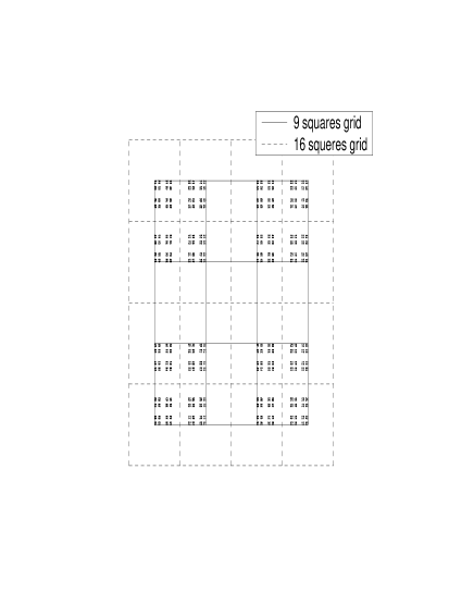
FIG. 1.: $2D$ Cantor set. Two different positions of the two dimensional grid, give completely different FD.

In some cases this average is not sufficient because several values of $I_{q}(\varepsilon)$ can be computed for the same $\varepsilon$. To illustrate this we use a $2D$ Cantor set, presented in Fig. 1. We start from a square. From 9 sub-squares we erase the 5 internal squares. We continue with this evolution for each remainder square. This procedure is continued, in principle, to infinity. The FD, $D_{0}$, of the $2D$ Cantor set is $\ln 4/\ln 3$ (when $q=0$, $I_{0}$ is just the number of nonempty squares and $D_{0}$ is the logarithmic ratio between nonempty squares and $\varepsilon$, where the square edge is normalized to one) as shown in Fig 1. However, it is possible to locate the $2D$ grid in such a way that there are 16 nonempty squares, giving rise to $D_{0}=2\ln 4/\ln 3$, twice the time of real FD of the system. This illustration shows that when $\varepsilon$ is not small, different positions of the grid can lead to different FD’s. In this case it is clear that we have to locate the grid in such a way that minimum squares will be nonempty (it is easy to show that this claim for the minimum is true for every $q$). In general, we can say that one must locate the hyper-grid so that the general information is minimum :

$$\tilde{I_{q}}(\varepsilon)\equiv\min\frac{1}{1-q}\ln(\sum_{i=1}^{M(\varepsilon)}p_{i}^{q}),$$ (5)

This proper location of the hyper-grid reduces the influence of surface boxes that are partly contained in the attractor. The requirement of a minimum gives a good estimate for the GID when $\varepsilon$ is not small.

B Generalized correlation dimension

In 1983 Grassberger and Procaccia presented a new method for calculating $D_{2}$ [14]. According to this method, it is possible to calculate dimension just from the correlation between different points, without direct connection to the phase space, and therefore easy to use. Some years later, a more general correlation function was suggested by Pawelzik and Schuster [15] :

$$C_{q}(r)=\Biggl{[}\frac{1}{N}\sum_{i=1}^{N}\biggl{[}\frac{1}{N}\sum_{j=1}^{N}\Theta\bigl{(}r-\left|\vec{x}_{i}-\vec{x}_{j}\right|\bigr{)}\biggr{]}^{q-1}\Biggr{]}^{1\over q-1},$$ (6)

where $N$ is number of points, $\vec{x}_{i}$ is a point of the system and $q$ is the generalization. $\Theta(x)$ is the Heaviside step function

$$\Theta(x)=\left\{\begin{array}[]{ll}0&{\rm when~{}}x\leq 0\\ 1&{\rm when~{}}x>0.\end{array}\right.$$ (7)

According to this method we have to calculate the generalized probability to find any two points within a distance $r$. This method is some kind of integration on eq. (2). It is not necessary to compute the real distance (e.g. $\left|\left|\vec{x}\right|\right|=\sqrt{x_{1}^{2}+\cdots+x_{n}^{2}}$ where n is the phase space dimension); it is equivalent to calculating the probability to find any two points in a hyper-box where one of them is located in the middle (e.g. $\left|\left|\vec{x}\right|\right|=\max_{1\leq i\leq n}\left|x_{i}\right|$ [16]). It is easier to compute the last possibility. For the special case of $q=1$, eq. (6) can be written (by applying the l’Hospital’s rule [10]) as :

$$\ln C_{1}(r)=\frac{1}{N}\sum_{i=1}^{N}\ln\biggl{[}\frac{1}{N}\sum_{j=1}^{N}\Theta\bigl{(}r-\left|\vec{x}_{i}-\vec{x}_{j}\right|\bigr{)}\biggr{]}.$$ (8)

The generalized correlation dimension (GCD) has a similar definition to the GID (eq. (4)) :

$$D_{q}=\lim_{N\to\infty;r\to 0}\frac{\ln C_{q}(r)}{\ln r}.$$ (9)

Both GID and GCD methods should give identical results. The GCD method is easy use and gives smooth curves. On the other hand, the method requires $O(N^{2})$ computations. Also, the smooth curves due to averaging over all distances are associated with a loss in information based on the attractor structure.

As we pointed out earlier, we usually have a limited number of points, forcing us to calculate dimension at large $r$. Thus an error enters the calculation of FD. The minimum number of points needed for the FD calculation has been discussed in several papers and different constraints suggested (for example [18] and [19]). In this paper we will use the $N_{min}$ of the Eckmann and Ruelle [19] constraint :

$$D_{2}<\frac{2\log_{10}N}{\log_{10}\Bigl{(}\frac{1}{\rho}\Bigr{)}},$$ (10)

under the following conditions :

$$\rho=\frac{r}{r_{0}}\ll 1\qquad\frac{1}{2}N^{2}\rho^{D}\gg 1,$$ (11)

with reference to Grassberger and Procaccia method. Here, $r_{0}$ is the attractor diameter, and $r$ is the maximum distance that gives reliable results in eq. (6) when $q=2$. The normalized distance, $\rho$, must be small because of the misleading influence of the hyper-surface. A $\rho$ too large (close to 1) can cause incorrect results since we take into account also hyper-boxes that are not well occupied because the major volume is outside the attractor.

However, if one has a long time series, then it is not necessary to compute all $N^{2}$ relations in eq. (6). One can compute eq. (6) for certain reference points such that the conditions in eq. (11) will still hold. Then, eq. (6) can be written as follows :

$$C_{q}(r) = \Biggl{[}\frac{1}{N_{ref}}\sum_{i=1}^{N_{ref}}\biggl{[}\frac{1}{N_{data}-2w-1}\times$$ (13)

$$\sum_{j=1}^{N_{data}}\Theta\bigl{(}r-\left|\vec{x}_{i\cdot s}-\vec{x}_{j}\right|\bigr{)}\biggr{]}^{q-1}\Biggr{]}^{1\over q-1},$$

where

$$\left|i\cdot s-j\right|>w\qquad s={\lfloor{\frac{N_{data}}{N_{ref}}}\rfloor}.$$

For each reference point we calculate the correlation function over all data points. The step for the time series is $s$. To neglect short time correlation one must also introduce a cutoff, $w$. Usually $w\approx m$ ($m$ corresponds to the $\tau$ from (1)) [20]. The number of distances $\left|\vec{x}_{i}-\vec{x}_{j}\right|$ will be $P=N_{ref}(N_{data}-2w-1)$ instead of $N^{2}$. The new form of eq. (10) is:

$$D<\frac{\log_{10}P}{\log_{10}\Bigl{(}\frac{1}{\rho}\Bigr{)}},$$ (14)

and the conditions (11) become

$$\rho=\frac{r}{r_{0}}\ll 1\qquad\frac{1}{2}P\rho^{D}\gg 1.$$ (15)

Although we discussed here a minimum number of data points needed for the dimension calculation, one must choose $\rho$ such that the influence from the surface is negligible (the growth of the surface is exponential to the embedding dimension). That gives us an upper limit for $\rho$. On the other hand, in order to find the FD we must average over a range of $r$, giving us a lower limit for $\rho$; therefore $N_{min}$ is determined according to the lower limit, giving rise to larger amount of points.

III Algorithm

A Background

In this section we describe an algorithm for GID method. The algorithm is based on a string sort and can be useful both for GID and GCD methods.

In previous works there have been several suggestions to compute DIG [21, 22, 23, 24, 25, 26]. The key idea of some of those methods [23, 24, 25] is to rescale the coordinates of each point and to express them in binary form. Then, the edge-box size can be initialized by the lowest value possible and then double it each time. Those methods require $O(N\log N)$ operations. Another method [22] uses a recursive algorithm to find the FD. The algorithm starts from a $d$ dimensional box which contains all data points. Then, this box is divided into $2^{d}$ sub boxes, and so on. The empty boxes are not considered, and those which contain only one point are marked. This procedure requires only $O(N)$ operations (for a reasonable series length this fact does not make a significant difference [22]).

As pointed out in ref. [22], in spite of the efficiency of the above algorithm (speed and resolution), it is quite difficult to converge to the FD of a high dimensional system. We were aware to this difficulty, and suggested a smoothing term to solve it (as will be explained in this section). Basically, we allow any choice of edge length (in contrast to power of 2 edge size of the above methods) and optimal location of the grid is searched. This procedure leads to convergence to the FD.

One of the works that calculates GID was done by Caswell and Yorke [21]. They calculate FD of $2D$ maps. They have proved that it is very efficient to divide the phase space into circles instead of squares in spite of the neglected area between the circles. However, this approach is not suitable for higher phase space dimensions. The reason might be that the volume of the hyper-balls compared to the entire volume of the attractor decreases according to the attractor dimension, and in this way we lose most of the information that is included in the attractor, since the space between the hyper-balls is not taken into account. It is easy to show that the ratio between the volume of the hyper-sphere with radius $R$, $V_{S}$, and the volume of the hyper-box with edge size of $2R$, $V_{B}$ (the sphere is in the box), is

$$\frac{V_{S}(2n)}{V_{B}(2n)}=\frac{1}{2\cdot 4\cdot 6\cdots 2n}\Bigl{(}\frac{\pi}{2}\Bigr{)}^{n},$$ (16)

for even phase space dimension, and,

$$\frac{V_{S}(2n-1)}{V_{B}(2n-1)}=\frac{1}{1\cdot 3\cdot 5\cdots(2n-1)}\Bigl{(}\frac{\pi}{2}\Bigr{)}^{n-1},$$ (17)

for odd phase space dimension. It is clear that the ratios (16) and (17) tend to zero for large $n$.

B Algorithm

Let us call the time series $x(i)$. The form of the reconstructed vector, (1), depends on the jumping, $m$, that creates the phase space. We order the time series in the following way :

$$\left.\begin{array}[]{l}x(0),x(m),x(2m),\ldots,x((l-1)m),\\ x(1),x(1+m),x(1+2m),\ldots,x(1+(l-1)m),\\ \vdots\\ x(m-1),x(m-1+m),\ldots,x(m-1+(l-1)m),\\ \end{array}\right.$$ (18)

where $l=\lfloor\frac{N_{p}}{m}\rfloor$. Let us denote the new series as $\tilde{x}_{i}$ ($i=0\ldots(lm-1)$; we lost $N_{p}-lm$ data points). If we take $n$ consecutive numbers in each row, we create a reconstructed vector in the $n$ dimensional embedding dimension.

At this stage, we fit a string (for each $\varepsilon$) to the number series (18). One character is actually a number between $0\ldots 255$, and thus, it is possible to divide one edge of the hyper-box to 255 parts (we need one of the 256 characters for sign). The correspondence is applied in the following way. We search for the minimum value in $\tilde{x}_{i}$ series, and denote it as $\tilde{x}_{min}$ (similarly, we denote the maximum values as $\tilde{x}_{max}$). The corresponding character to $\tilde{x}_{i}$ is :

$$y_{i}=\lfloor\frac{\tilde{x}_{i}-\tilde{x}_{min}}{\varepsilon}\rfloor.$$ (19)

The value of $\varepsilon$ is in the range

$$\frac{(\tilde{x}_{max}-\tilde{x}_{min})}{255}\leq\varepsilon\leq(\tilde{x}_{max}-\tilde{x}_{min}).$$ (20)

If we take now $n$ consecutive characters (string), we have the “address” of the hypercube in which the corresponding vector is found.

Let us represent the string as follows :

$$\left.\begin{array}[]{l}s_{0}=y_{0}y_{1}\ldots y_{n-1},s_{1}=y_{1}\ldots y_{n},\ldots,s_{l-n}=y_{l-n}\ldots y_{l-1},\\ s_{l-n+1}=y_{l}\ldots y_{l+n-1},\ldots,s_{2(l-n)+1}=y_{2l-n}\ldots y_{2l-1},\\ \vdots\\ s_{(m-1)(l-n+1)}=y_{(m-1)l}\ldots y_{(m-1)l+n-1},\ldots,\\ \qquad\qquad\qquad\qquad\qquad s_{m(l-n+1)-1}=y_{ml-n}\ldots y_{ml-1}.\\ \end{array}\right.$$ (21)

Obviously, we do not have to keep each string $s_{i}$ in the memory; we can keep just the pointers to the beginning of the strings in the characters series, $y_{i}$. The number of vectors / strings is $m(l-n+1)$.

As mentioned, each string is actually the address of a hyper-box (which the vector is in it) in a hyper-grid that cover the attractor. The first character is the position of the first coordinate of the hyper-box on the first edge of the hyper-grid. The second character denotes the location on the second edge, and so on. We actually grid the attractor with a hyper-grid so that any edge in this grid can be divided into 255 parts. Thus the maximal number of boxes is $255^{n}$, where $n$ is the embedding dimension (there is no limit for $n$). Most of those boxes are empty, and we keep just the occupied boxes in the hyper-grid.

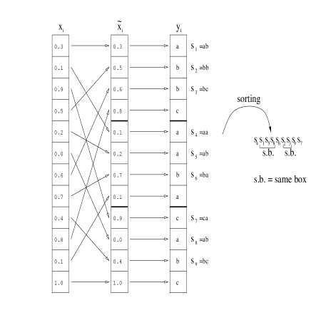
FIG. 2.: Illustration of the GID algorithm. We take series containing $12$ data points between zero and one. The parameter values are: $m=3$, $\varepsilon=0.4$ and $n=2$. For simplicity we assume that the lowest character is ’a’.

The next step is to check how many vectors fall in the same box, or, in other words, how many identical “addresses” there are. For this we have to sort the vector that points to strings, $s_{i}$, in increasing order (one string is less then other when the first character that is not equal is less then the parallel character; e.g., ’abcce’$<$’abcda’ since the fourth character in the first string, c, is less then the fourth character in the second string, d). The above process is illustrated in Fig. 2.

The most efficient way to sort $N$ elements is the “quick sort” [27, 28]. It requires just $O(N\log_{2}N)$ computations. However, this sort algorithm is not suitable for our propose, since after the vector is sorted, and we slightly increase the size of the edge of the hyper-box, $\varepsilon$, there are just a few changes in the vector, and most of it remains sorted. Thus, one has to use another method which requires less computations for this kind of situation, because the quick sort requires $O(N\log_{2}N)$ computations independently of the initial state. The sort that we used was a “shell sort” [27], which requires $O(N^{3/2})$ computations in worst case, around $O(N^{5/4})$ computations for random series, and $O(N)$ operations for an almost sorted vector. Thus, if we compute the information function for $m$ different $\varepsilon$ values $O(N\log_{2}N+mN)$ operations will be needed.

After sorting we count how many identical vectors there are in each box. Suppose that we want to calculate GID for embedding dimensions $n_{min}\ldots n_{max}$, and generalizations $q_{min}\ldots q_{max}$. We count in the sorted pointers vector identical strings containing $n_{max}$ characters. Once we detect a difference we know that the coordinate of the box has changed. We detect the first different location. First difference in the last character of the string means that it is possible to observe the difference just in the $n_{max}^{th}$ embedding dimension, and in lower embedding dimension it is impossible to observe the difference. If the first mismatch is in the $n^{th}$ character in the string, then the box changes for embedding dimensions higher than or equal to $n$. We hold a counter vector for the different embedding dimensions, and we will assign zero for those embedding dimensions in which we observed a change. In this stage, we have to add to the results matrix the probability to fall in a box according to eqs. (2), (3). We continue with this method to the end of the pointer vector and then print the results matrix for the current $\varepsilon$ and continue to the next $\varepsilon$.

It is easy to show that one does not have to worry about the range of the generalization, $q$, because for large time series with $10^{6}$ data points the range of computational $q$’s is -100..100.

The method of string sorting can be used also for calculating GCD. Our algorithm is actually a generalization of the method that was suggested by Grassberger [16]. The algorithm is specially efficient for small $r$ ($r<\frac{1}{10}D$ where $D$ is the attractor diameter) and it requires $O(N\log_{2}N)$ computations instead of $O(N^{2})$ computations (according to the Grassbeger algorithm it requires $O(N)$ computations instead $O(N^{2})$ computations).

The basic idea of Grassberger was that for small $r_{max}$ values, where $r_{max}$ is the maximum distance for which the correlation function is computed, one does not have to consider distances larger then $r_{max}$, distances which require most of the computation time. Thus, it is enough to consider just the neighboring boxes (we use the definition distance $\left|\left|\vec{x}\right|\right|=\max_{1\leq i\leq n}\left|x_{i}\right|$ in eq. (6)), for which their edge is equal to $r_{max}$, since distances greater then $r_{max}$ are not considered in eq. (6). If, for example, one wants to calculate the correlation of $r\leq r_{max}=\frac{1}{10}D$ (in accordance with conditions (10) (11) (14) (15)), then (in $2D$ projection) it is enough to calculate distances in 9 squares instead 100 squares (actually, it is enough to consider just 5 squares since eq. (6) is symmetric). According to Grassberger, one has to build a matrix for which any cell in it points to the list of data points located in it. It is possible to generalize this method to a $3D$ projection matrix.

The generalization to higher dimensions can be done very easily according to the string sort method. As a first step one has to prepare a string $y_{i}$ (19), which is the same operation as gridding the attractor by a hyper-grid of size $r$. The next step is to sort strings $s_{i}$ (21). For each reference point in eq. (13) the boxes adjoining the box with the reference point in it should be found. Now, it is left to find the distances between the reference point to other points in neighboring boxes (we keep the pointer vector from string $y_{i}$ to the initial series and vice versa), and calculate the correlation according to eq. (13).

The algorithm described above is especially efficient for very complex systems with high FD. For example, for EEG series produce by brain activity, it well known (except for very special cases such as epilepsy [17]) that the FD is, at least, four. In this case $n_{min}=4$, and instead of calculating distances in $l^{4}$ boxes ($l$ is the ratio between the attractor diameter and $r$) it is sufficient to calculate distances in $3^{4}=81$ boxes. If, for example, $l=9$, just $3^{4}/9^{4}=\frac{1}{81}$ distances must be computed (or even less if one take into account also the symmetry of eq. (13)). In this way, despite the $O(N\log_{2}N)$ operations needed for the initial sort, one can reduce significantly the computation time.

C Testing of GID algorithm and number of data points needed for calculating GID

Let us test the algorithm of GID on random numbers. We create a random series between 0 to 1 (uniform distribution). We then reconstruct the phase space according to Takens theory (1). For any embedding dimension that we would like to reconstruct, the phase space we will get a dimension that is the same as the embedding dimension, since the new reconstructed vectors are random in the new phase space, and hence fill the space (in our case, a hyper-cube of edge 1).

For embedding dimension 1 (a simple line), if the edge length is $\varepsilon$, then the probability to fall in any edge is also $\varepsilon$. The number of edges $\varepsilon$ that covers the series range $[0,1)$ is $\lfloor\frac{1}{\varepsilon}\rfloor$. The probability to fall in the last edge is $1\%\varepsilon$ (the residue of the division). For generalization $q$ one gets :

$$\sum_{i=1}^{M(\varepsilon)}p_{i}^{q}=\lfloor 1/\varepsilon\rfloor\varepsilon^{q}+(1\%\varepsilon)^{q}.$$ (22)

For embedding dimension 2, one has to square (22) since the probability distribution on different sides is equal. For embedding dimension $n$ eq. (2) becomes :

$$I_{q}(\varepsilon)=\frac{1}{1-q}\ln[\lfloor 1/\varepsilon\rfloor\varepsilon^{q}+(1\%\varepsilon)^{q}]^{n}.$$ (23)

Opening eq. (23) according to the binomial formula will give all different combinations for the partly contained boxes. Notice that this grid location fulfills requirement (5) for the minimum information function.

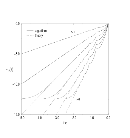
FIG. 3.: Dimension calculation for random series by GID algorithm and by the theory.

In Fig. 3 we present $-I_{2}(\varepsilon)$, both, according to the GID algorithm, and according to eq. (23). There is full correspondence between the curves, and, as we find, it is possible to see that the slope (dimension) in the embedding dimension $n$ is equal to the dimension itself. When $-I_{2}(\varepsilon)\approx-10$, the curves separate. There is lower convergence (when $-I_{2}(\varepsilon)\approx-12.5$) since the edge is too small, and the number of reconstructed vectors is equal to the number of nonempty boxes.

The “saw tooth” that seen in Fig. 3 caused by partial boxes that fall on the edge of the hyper-box. The “saw tooth” appears when there is an integer number of edges that covers the big edge. The slope in the beginning of every saw tooth is equal to zero (that comes from the extremum condition of (23)). The “saw teeth” become smaller when $\varepsilon$ decrease, since the relative number of boxes that fall on the surface in small compared to the entire number of boxes.

It is possible to calculate roughly the number of points needed for the dimension calculation in a homogeneous system. The separation point of Fig. 3 is approximately around $-I_{2}(\varepsilon)\approx-10$, for every embedding dimension. Thus, the number of hyper-boxes at this point is $e^{10}$ (since $-10=\ln\left(M(\varepsilon)p^{2}\right)$ where $p\sim\frac{1}{M(\varepsilon)}$ in our example). The graph come to a saturation around $-I_{2}(\varepsilon)\approx-12.5$, giving rise to $e^{12.5}$ data points. The number of points per box is just, $e^{2.5}\approx 12$. Thus, generally, when there are less then 12 points per box, the value of $I_{q}(\varepsilon)$ is unreliable. Let us denote the minimum edges needed for the calculation as $m_{min}$ ($m_{min}$ is just $\lfloor 1/\varepsilon\rfloor$, and thus one can define a lower value for $\varepsilon$). The number of hyper-boxes in embedding dimension $n$ is $m_{min}^{n}$. Thus, the minimum number of points needed for computing the FD of an attractor with an FD $D$, is:

$$N=12m_{min}^{D}.$$ (24)

This estimate is less then what was required by Smith [18] ($42^{D}$) and larger then the requirement of Eckmann and Ruelle [19] (if we take, for example, $m_{min}={\frac{1}{\rho}}=10$ then according to (10) $10^{D/2}$ points is needed and according to (24) $12\times 10^{D}$ points is needed). However, as we pointed out earlier, (24) is a rough estimation, and one can converge to a desired FD even with less points.

IV Examples

In this section we will present the results of both GID and GCD on well known systems, such as the Lorenz attractor and the Rossler attractor. The FD of those results are well known by various methods, and we will present almost identical results achieved by our methods. In the following examples, we choose one of the coordinates to be the time series; we normalize the time series to be in the range of $0\ldots 1$.

A Lorenz Attractor

The Lorenz attractor [29] is represented by a set of three first order non-linear differential equations :

$${dx\over dt} = \sigma(y-x)$$ (25)

$${dy\over dt} = -xz+rx-y$$ (26)

$${dz\over dt} = xy-bz.$$ (27)

Although it is much simpler to find the FD from the real phase-space $(x,y,z)$, we prefer the difficult case of finding the FD just from one coordinate to show the efficiency of Takens theorem. We choose the $z^{th}$ component to be the time series from which we reconstruct the phase space (the parameter values are: $\sigma=16$, $r=45.92$, $b=4$). We took $32768$ data points and $m=6$ (the jumping on the time series which creates the reconstructed phase space; the time step is $\Delta t=0.02$). The generalization that we used was $q=2$. The embedding dimensions were $n=1..7$. The FD of Lorenz attractor is $2.07$ ([30] and others).

In Fig. 4 we show the results of GCD and GID methods. As expected from the GCD curves, in Fig. 4a we see very smooth curves, for which the slopes (in the center parts of the curves) converge approximately to dimension $2.08$. In Fig. 4b we see some jumping in the GID curves. It can be clearly seen that for small $\varepsilon$, one can not see the jumping while for large $\varepsilon$ the non-monotonicity is much stronger. This is typical behavior for GID curves; large $\varepsilon$ (or larger box edge) reflects more variability of $-I_{2}(\varepsilon)$ to the hype- grid location. To smooth the curves in order to get reliable results, it is necessary to find a proper location of the hyper-grid that gives minimum general information $\tilde{I}_{2}(\varepsilon)$ (or maximum $-\tilde{I}_{2}(\varepsilon)$). We have performed 7 comparisons to find that proper location. As for GCD, we also fitted approximate linear curves (dashed lines) which lead to dimension $2.09$ (Fig. 4c), and thus, agree well with previous results. To make sure of the validity of the dimension results we add here (Fig. 4d) graphs of successive slopes of curves in Fig. 4c, and conclude with dimension results versus embedding dimension according to several generalizations ($q=2..5$, Fig. 4e). In both graphs, the approximate dimension is $2.03$.

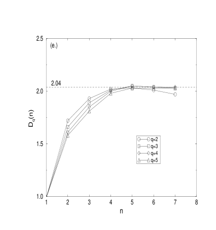
FIG. 4.: Correlation and information curves of reconstructed Lorenz attractor. a. Correlation curves; the estimate slopes are added. b. Unsmoothed information curves. c. Smoothed information curves; the estimated linear curves (dashed line) and their slope is added. d. The slopes of $-\tilde{I}_{2}(\varepsilon)$ (Fig. 4c). The dashed line represents the estimated FD. e. FD of Lorenz attractor for different embedding dimensions, $n$, and for different generalizations, $q$.

B Rossler Attractor

Let us examine briefly our second example, the Rossler attractor [31]. The differential equations which generate the trajectory are :

$$\frac{dx}{dt} = -z-y$$ (28)

$$\frac{dy}{dt} = x+ay$$ (29)

$$\frac{dz}{dt} = b+z(x-c).$$ (30)

The parameter values are : $a=0.15$, $b=0.2$, $c=10$. The time step is $t=0.2$ and $m=8$. We use the $y$ direction to be the time series. The number of data points is $N=16384$. In Fig. 5 we show the results of GID method of embedding dimension $n=1..7$. There are many more discontinuities in the unsmoothed curves (Fig. 5a) compared to the Lorenz attractor, reflecting a sensitivity to the grid location. The smooth curves in Fig. 5b are produced after 20 comparisons. Again, we approximate the slopes of central linear part of the curves in two different ways and find dimension $2.05$, which is in agreement with dimension $2.03$ calculated by the use of the GCD method, and through the Lyapunov exponent [30].

FIG. 5.: a. Unsmoothed graphs of Rossler attractor. b. Smoothed information graphs; the FD estimation is added.

C Van der Pol Oscillator

Another example that will be tested is the van der Pol oscillator [32]. This system was investigated in the beginning of the century in order to find a model for the heart beat variability (among other uses of this equation). The behavior of the system (with parameter values that will be used) is chaotic although it looks quite periodic. Thus, we expect a smooth behavior of the geometrical structure of the attractor. The equation of motion is :

$${\ddot{x}}-\alpha(1-x^{2})\dot{x}+kx=f\cos\Omega t.$$ (31)

The parameter values are : $\Omega=2.446$, $\alpha=5$, $k=1$ and $f=1$. Habib and Ryne [33] and others [34] have found that the Lyapunov exponents of the system are $\lambda_{1}\approx 0.098$, $\lambda_{2}=0$ and $\lambda_{3}\approx-6.84$, and thus, according to the Kaplan and Yorke formula [2],

$$D_{L}=j+{\sum_{i=1}^{j}\lambda_{i}\over|\lambda_{j+1}|}\approx 2+{0.098\over 6.84}\approx 2.014$$ (32)

where $j$ is defined by the condition that $\sum_{i=1}^{j}\lambda_{i}>0$ and $\sum_{i=1}^{j+1}\lambda_{i}<0$. The fact that the system has a “periodic” nature is reflected in this very low FD (as known, the minimal FD of a chaotic system is 2).

FIG. 6.: van der Pol oscillator : The smoothed information graphs, $-\tilde{I}_{1}(\varepsilon)$; The estimated FD is added (dashed lines with their corresponding slope).

In Fig. 6 we present the calculation of $D_{1}$ which we suppose to be close to $D_{L}$. The approximate slope lead to an FD of $D_{1}\sim 2.02$, which is in good agreement to $D_{L}$. Notice that minimization of $I_{1}(\varepsilon)$ did not succeed for large $\varepsilon$ values although we used 7 grid comparisons; that fact can cause a small error in the slope estimation, since usually the slope is determined from the central part of the curves.

D Mackey-Glass Equation

Up to now we examined the relation between GID and GCD on systems with finite dimension, for which their FD can be calculated by using methods based on the true integrated vector of the system. A class of systems which is more close to reality are systems with infinite dimensional dynamics. A delay differential equation of the type

$$\frac{dx(t)}{dt}=F(x(t),x(t-\tau))$$ (33)

belongs to this class. In order to solve this kind of equation, one needs to initiate $x(t)$ in the range $0\leq t\leq\tau$, and then, by assuming that the system can be represented by a finite set of discrete values of $x(t)$, it is possible to evaluate the system dynamics step by step. The solution is considered to be accurate if one converges to the same global properties, such as, Lyapunov exponents and FD, by different methods [35], and without dependence on the number of intervals to which the function is divided [14]. Delay equations, such as eq. (33), describe systems in which a stimulus has a delay response. There are many practical examples from control theory, economics, population biology, and other fields.

One of the known examples is the model of blood cell production in patients with leukemia, formulated by Mackey and Glass [38] :

$$\dot{x}(t)=\frac{ax(t-\tau)}{1+[x(t-\tau)]^{c}}-bx(t).$$ (34)

Following refs. [35, 14], the parameter values are : $a=0.1$, $b=0.2$, and $c=10$. We confine ourselves to $\tau=30.0$. As in ref. [14], we choose the time series to be $\{x(t),x(t+\tau),x(t+2\tau),\ldots\}$, as well as the integration method which is described in this reference. The length of the time series is $N=131072$.

FIG. 7.: Mackey-Glass equation: a. The GCD graphs. One notices two regions of parallel curves, which lead to different FD’s. b. The successive slopes of a. c. The GID graphs. d. The successive slopes of c.

The FD ($D_{2}$) calculation of the Mackey-Glass equation is presented in Fig. 7. The embedding dimensions are, $n=1\ldots 9$. In Fig. 7a, the correlation function, $C_{2}(r)$ is shown. One notices that there are two regions in each one of which there is convergence to a certain slope. These regions are separate by a dashed line. In Fig. 7b, the average local slope of Fig. 7a is shown. One can identify easily two convergences, the first in the neighborhood of $\sim 3.0$, and the second around $\sim 2.4$. Thus, there are two approximations for the FD, $D_{2}$, pointing to two different scales. The first approximation is similar to the FD that was calculated in ref. [14]. However, the GID graphs which are presented in Fig. 7c and d lead to an FD, $D_{2}\sim 2.45$, which seems to be very close to the second convergence of Fig. 7b. Notice that the convergence to $D_{2}\sim 2.4$ appears, in both methods, in the neighborhood of the same box size ($\sim 2.1$).

V Summary

In this work we develop a new algorithm for calculation of a general information, $I_{q}(n)$, which is based on strings sorting (the method of string sort can be used also to calculate the conventional GCD method). According to our algorithm, one can divide the phase space into 255 parts in each hyper-box edge. The algorithm requires $O(N\log_{2}N)$ computations, where $N$ is the number of reconstructed vectors. A rough estimate for the number of points needed for the FD calculation was given. The algorithm, which can be used in a regular system with known equations of motion, was tested on a reconstructed phase space (which was built according to Takens theorem). The general information graphs have non monotonic curves, which can be smoothed by the requirement for minimum general information. We examine our algorithm on some well known examples, such as, the Lorenz attractor, the Rossler attractor, the van der Pol oscillator and others, and show that the FD that was computed by the GID method is almost identical to the well known FD’s of those systems.

In practice, the computation time of an FD using the GID method, was much less than for the GCD method. For a typical time series with $32768$ data points, the computation time needed for the GCD method was about nine times greater than the computation time of GID method (when we do not restrict ourselves to small $r$ values and we compute all $N^{2}$ relations). Thus, in addition to the fact that the algorithm developed in this paper enables the use of comparative methods (which is crucial in some cases), the algorithm is generally faster.

The author wishes to thank J. Levitan, M. Lewkowicz and L.P. Horwitz for very useful discussions.

REFERENCES

- [1]
- [2] J.L. Kaplan and J.A. Yorke, in: Functional Differential Equations and Approximations of Fixed Points, Lecture Notes in Mathematics 730, eds. H.-O. Peitgen and H.-O. Walther (Springer Verlag, Berlin, 1979).
- [3] A. Babloyantz, C. Nicolis, and M. Salazar, Phys. Rev. A 111, 152 (1985); A. Babloyantz and A. Destexhe, Proc. Natl. Acad. Sci. USA 83 3513 (1986).
- [4] E. Basar, ed., Chaos in the Brain (Springer, Berlin, 1990).
- [5] G. Mayer-Kress, F.E. Yates, L. Benton, M. Keidel, W.S. Tirsch and S.J. Poepple, Math. Biosci. 90, 155 (1988).
- [6] K. Saermark, J. Lebech, C.K. Bak, and A. Sabers, in: Springer Series in Brain Dynamics, 2 eds. E Basar and T.H. Bullock (Springer, Berlin, 1989) p. 149.
- [7] K. Saermark, Y. Ashkenazy, J. Levitan, and M. Lewkowicz, Physica A 236, 363 (1997).
- [8] F. Takens, in : Dynamical Systems and Turbulence, eds. D. Rand and L.S. Young, (Springer Verlag, Berlin, 1981).
- [9] Discussions about the choose of see for example : H.G. Schuster, Deterministic Chaos, (Physik Verlag, Weinheim, 1989); A.M. Fraser and H.L. Swinney, Phys. Rev. A 33, 1134 (1986); J.-C. Roux, R.H. Simoyi and H.L. Swinney, Physica D 8, 257 (1983).
- [10] H.D.I. Abarbanel, R. Brown, J.J. Sidorowich, and L.S. Tsimring, Rev. Mod. Phys. 65, 1331 (1993).
- [11] M. Ding, C. Grebobi, E. Ott, T. Sauer and J.A. Yorke, Physica D 8, 257 (1993).
- [12] C.E. Shannon and W. Weaver, The Mathematical Theory of Information, (University of Ill. Press, Urbana, 1949).
- [13] J. Balatoni and A. Renyi, in : Selected Papers of A. Renyi, ed. P. Turan, (Akademiai K. Budapest, 1976), Vol. 1, p. 588.
- [14] P. Grassberger and I. Procaccia, Physica D 9, 189 (1983).
- [15] K. Pawelzik and H.G. Schuster, Phys. Rev. A 35, 481 (1987).
- [16] P. Grassberger, Phys. Lett. A 148, 63 (1990).
- [17] A. Babloyantz and A. Destexhe, in: From Chemical to Biological Organization, eds. M. Markus, S. Muller, and G. Nicolis (Springer Verlag, Berlin, 1988).
- [18] L.A. Smith, Phys. Lett. A 133, 283 (1988).
- [19] J.-P. Eckmann and D. Ruelle, Physica D 56, 185 (1992).
- [20] J. Theiler, Phys. Rev. A 34, 2427 (1986).
- [21] W.E. Caswell and J.A. York, in: Dimensions and Entropies in Chaotic Systems, ed. G. Mayer-Kress, (Springer Verlag, Berlin, 1986).
- [22] T.C.A. Molteno, Phys. Rev. E 48, 3263 (1993).
- [23] X.-J. Hou, R. Gilmore, G. Mindlin, and H. Solari, Phys. Lett. A 151, 43 (1990).
- [24] A. Block, W. von Bloh, and H. Schnellnhuber, Phys. Rev. A 42, 1869 (1990).
- [25] L. Liebovitch and T. Toth, Phys. Lett. A 141, 386 (1989).
- [26] A. Kruger, Comp. Phys. Comm. 98, 224 (1996).
- [27] W.H. Press, S.A. Teukolsky, W.T. Vetterling, and B.P. Flannery, Numerical Recipes in C, 2nd edn. (Cambridge University, Cambridge, 1995).
- [28] D.E. Knooth, The Art of Computer Programming vol. 3 - Sorting and Searching, (Addison-Wesley, Reading, Mass., 1975); There is other sort algorithms that require even less computation () such as radix sorting, A.V. Aho, J.E. Hopcroft, and J.D. Ullman, Data Structures and Algorithms, (Addison-Wesley, Mass., 1983).
- [29] E.N. Lorenz, J. Atmos. Sci. 20, 130 (1963).
- [30] A. Wolf, J.B. Swift, H.L. Swinney and J.A. Vastano, Physica D 16, 285 (1985).
- [31] O.E. Rossler, Phys. Lett. 57A, 397 (1976).
- [32] B. van der Pol, Phil. Mag. (7) 2, 978 (1926); B. van der Pol and van der Mark, Phil. Mag. (7) 6, 763 (1928).
- [33] S. Habib and R.D. Ryne, Phys. Rev. Lett. 74, 70 (1995).
- [34] K. Geist, U. Parlitz, and W.Lauterborn, Prog. Theor. Phys. 83, 875 (1990).
- [35] J.D. Farmer, Physica D 4, 366 (1981).
- [36] J.M. Greene, J. Math. Phys. 20, 1183 (1979).
- [37] Y. Ashkenazy, C. Goren, and L.P. Horwitz, Phys. Lett. A, 243, 195 (1998).
- [38] M.C. Mackey and L. Glass, Science 197, 287 (1977).