Abstract

Unidirectionally coupled dynamical system is studied by focusing on the input (or boundary) dependence. Due to convective instability, noise at an up-flow is spatially amplified to form an oscillation. The response, given by the down-flow dynamics, shows both analogue and digital changes, where the former is represented by oscillation frequency and the latter by different type of dynamics. The underlying universal mechanism for these changes is clarified by the spatial change of the co-moving Lyapunov exponent, with which the condition for the input dependence is formulated. The mechanism has a remarkable dependence on the noise strength, and works only within its medium range. Relevance of our mechanism to intra-cellular signal dynamics is discussed, by making our dynamics correspond to the auto-catalytic biochemical reaction for the chemical concentration, and the input to the external signal, and the noise to the concentration fluctuation of chemicals.

1 Introduction

In a biological system, signaling phenomena are important, that transform external inputs to outputs. In general the signaling process is not simple, and is not given by a fixed one-to-one correspondence. A typical example is an intra-cellular signaling, where several chemicals are involved. These chemicals include several catalytic reactions and positive feedback process to amplify the input. As a result nonlinear dynamics of coupled elements is concerned.

In a cell, an external stimulus coming from the outside of a cell is selected, amplified, and transported as a signal. Recent development in molecular biology provides us more and more detailed information on the signaling process[1]. In the experiment of molecular biology, mechanisms on chemical signal transmission have become clearer. Network of the pathways from a given stimulus through signal chemicals to the final response is also being clarified.

The network of signaling pathway is generally very much complicated. A large number of biochemical reactions are involved, from the cell membrane to ligand, and to the final response reaction. Often, the pathway may not be uni-directional, but several pathways interfere with each other. With this complication one could even expect that there would be no correlation between input and final response. If such were the case, however, no biological function would be expected. Then, why is the network of signal pathway so long and complicated? How can the signal pathway respond suitably to inputs? How does the signal process work within possible thermodynamic fluctuations?

To answer such general questions, experimental molecular biology is not sufficient, but some theoretical study on general features of a biosystem is required. To address the above questions, we start from a study of simple model pathway formed uni-directionally, as an ideal simplification of the signal pathway, where a model with a sequence of biochemical reactions from an input is adopted, that transforms input to the final response. Here we do not take a biologically realistic model, but focus on a dynamical system aspect abstracted by a simple model. With this we will propose a mechanism how a signal is amplified and transmitted within fluctuations.

To understand the mechanism of signaling, we note that the signal system should satisfy at least the following three properties;

property 1

: Amplification and transmission of input ; external signal is amplified and transmitted into an intra-cellular dynamics.

property 2

: (Linear) stability : the system returns to the original state when the input is off.

property 3

: Input dependence : response following the internal dynamics depends on the nature and strength of the input signal.

In the present paper, we introduce an abstract model with a simple biochemical signal pathway, and show that its dynamics can satisfy the above three properties. A chain of coupled biochemical reactions represents the model. Indeed, in signal pathways, there are several chains of reactions, where by means of enzyme-catalyzed pathways, many biochemical reactions are driven in one direction, through coupling to energetically favorable hydrolysis of ATP to ADP and inorganic phosphate [1].

In a dynamical system with one-way coupling, an important notion is convective instability, where small perturbation is amplified to down-flow, although the system is linearly stable and provides a stationary state without such perturbation. We will show that the properties 1 and 2 are satisfied with this convective instability, as will be explained in the next section. It will be also shown that some of the one-way coupled dynamical system with convective instability can have input dependence.

Here we consider a network of catalytic reaction elements, each of which is represented by differential equations showing excitatory dynamics. Each element is assumed to be connected uni-directionally. In other words, each chemical at the $(i-1)$-th site has an influence at the next $i$-th level. To be specific, we choose the model,

$$\dot{\vec{X}^{i}}=\vec{F}(\vec{X}^{i},\vec{X}^{i-1})\\$$ (1)

with $\vec{X}^{i}=(x^{i},y^{i})$.

In the present model, the input is represented just as a boundary condition $\vec{X}^{0}=const.$, while the response is given by the dynamics at the down-flow $i\gg 1$. We will find input dependence, or in other words boundary-condition sensitivity, and clarify its mechanism in the term of convective instability.

Since a convectively unstable (CU) system is often sensitive to noise as described later, it is important to discuss how our signal transmission works in the presence of noise, due to chemical fluctuations. Indeed, it is shown that our mechanism works in the presence of noise, or rather it works best when the noise strength is of a medium size.

Although our motivation is originated in signaling phenomena, our formulation of input-dependent dynamics is generally applied to any uni-directional chain of dynamical systems. In this respect, the mechanism of analogue and digital input-dependence, as well as our formula for their condition, will have general applicability. It may include neural networks[2], optical networks[3], open fluid flow, and other chain network of dynamical systems.

The present paper is organized as follows. In §2, noise amplification by convective instability will be reviewed. In §3, a simple model using coupled chemical reactions is introduced for biological signaling pathway. In §4, input dependence in our model is presented, while its mechanism will be explained in §5 in connection with convective instability and its spatial change due to input signal. In §6, the relevance of the noise to the input dependence is described. It is shown that the input dependence is possible only within some range of noise amplitude. §7 is devoted to the discussion and the conclusion.

2 Convective instability in a one-way coupled system

2.1 convective instability

One-way coupled system is introduced[4, 5] as an abstract model for an open flow system, for example, in a fluid system. By spatial amplification of disturbance at upper flow, the dynamics increases its complexity, as it goes to down-flow[5, 6, 7]. This change of dynamics is often triggered by convective instability.

Convective instability expresses how some perturbation is amplified along a flow. If a system is ‘convectively unstable’ (CU), perturbation is spatially amplified and transmitted as in Fig.1. On the other hand, if a system is convectively stable (CS), perturbation at an upper flow is damped as it goes down-flow. Note that even if the perturbation is damped at each site (i.e., the system is linearly stable (LS) ), the system can be CU as shown in Fig.1.

Figure 1: Schematic representation of the evolution of perturbation

Convective instability is quantitatively characterized by co-moving Lyapunov exponent $\lambda_{v}$, Lyapunov exponent observed from the inertial system moving with the velocity $v$ [8, 9]. For a given state, if $\mathop{max}_{v}\lambda_{v}$ is positive, the state is convectively unstable. The convective stability is supported by $\mathop{max}_{v}\lambda_{v}<0$, distinguishable from linear stability, given by the condition $\lambda_{0}<0$. The co-moving Lyapunov exponent is usually applied to an attractor, where chaos with convective instability is characterized by the positivity of $\mathop{max}_{v}\lambda_{v}$. It is however applied to any state, to characterize its stability.

Since $\lambda_{v}$ characterizes the amplification of perturbation for the velocity $v$, the amplification per one lattice site is given by $\frac{\lambda_{v}}{v}$. Hence the amplification rate per one site is given by the spatial Lyapunov exponent $\lambda^{S}$[10];

$$\lambda^{S}=\mathop{max}_{v}\frac{\lambda_{v}}{v}$$ (2)

2.2 noise sustained structure in convectively unstable system

For a system with convective instability, noise plays an important role. When a system is linearly stable but convectively unstable, applied noise is spatially amplified and transmitted from up-flow to down-flow, until spatiotemporal structure is generated at the down-flow[4, 11]. This structure is different from that for a system without noise.

Mechanism of the structure formation is summarized as follows[8, 11]. Assume that noise is added to LS but CU fixed point. Around the fixed point, the noise is spatially amplified and transmitted from up-flow to down-flow. The more it goes to down-flow, the larger oscillation can appear, until some stationary dynamics (such as periodic oscillation) is generated for $i\gg 1$. As long as the noise is added at the most up-flow element ($i=0$), the down-flow dynamics remains same. This noise-induced structure in a convectively unstable system is a general feature in a one-way coupled system and important for our model. Of course, if the system is CS around the fixed points at all elements, noise is spatially damped, and no oscillation exists at the down-flow.

3 Model

As a simple signaling model, we choose a one-way coupled differential equations(OCDE), where differential equation of each element can be regarded to express the dynamics of biochemical reaction.

3.1 dynamics of a single element

As dynamics of a single element, we choose an auto-catalytic biochemical reaction system, consisting of activator $x$ and inhibitor $y$ (see Fig.2). In other words, there is a set of two chemical variables for chemical concentrations, represented by differential equations with two degrees of freedom.

Figure 2: Schematic representation of biochemical reaction of a single element

As a specific example, we choose the following model,

$$\left\{\begin{array}[]{ll}\dot{x}=f(x,y)\\ \dot{y}=g(x,y)\end{array}\right.$$ (3)

with

$$\left\{\begin{array}[]{ll}f(x,y)=x\left\{(1-x)ax-by\right\}+K\\ g(x,y)=y(cx-dy)+K\end{array}\right.$$ (4)

where the parameters $a,b,c,d$, and $K$ can be related with the rate constants of biochemical reaction. In the present paper, we set $K\ll 1$, $a,b,c,d\sim 1$ so that the system is satisfied with the three properties in §1. In the present case, the suppression of the catalytic process is provided by the term $(1-x)$ (where $x$ is between 0 and 1), but other forms like Michael-Menten’s can be adopted. Here details of the model are not important, and only the excitatory nature in the dynamics is necessary.

This single-element dynamics is chosen so that $(x,y)$ converges to a linearly stable fixed point $(x_{*},y_{*})$, where $f(x_{*},y_{*})=g(x_{*},y_{*})=0$. There is neither a stable limit cycle nor another fixed point besides the above fixed point.

3.2 one-way coupling

Assuming that the identical set of dynamics is set at each $i$-th node, the coupling from each node to the next node is introduced as the activation process of the $i$-th node by the activator of the $(i-1)$-th node. In other words, we assume that the activator chemical at the $i$-th node is catalyzed by the $(i-1)$-th activator. This leads to the following one-way coupled differential equations.

$$\left\{\begin{array}[]{ll}\dot{x^{i}}&=f(x^{i},y^{i},x^{i-1})\\ \dot{y^{i}}&=g(x^{i},y^{i})\end{array}\right.$$ (5)

$$\left\{\begin{array}[]{ll}f(x^{i},y^{i},x^{i-1})&=x^{i}\left\{(1-x^{i})(ax^{i}+\epsilon x^{i-1})-by^{i}\right\}+K+{\eta}^{i}_{x}\\ g(x^{i},y^{i})&=y^{i}(cx^{i}-dy^{i})+K+{{\eta}^{i}_{y}}\end{array}\right.$$ (6)

where $i$ denotes a spatial position or a level of signal pathway. Coupling constant $\epsilon$ corresponds to the rate constant of biochemical reaction between $(i-1)$-th activator and $i$-th activator, and $\eta$ represents white noise expressing concentration fluctuation of chemicals satisfying

$$\langle{\eta}^{j}_{p}(t){\eta}^{k}_{q}(t-\tau)\rangle_{t}={\delta}_{p,q}{\delta}_{j,k}\delta(\tau)\sigma^{2}$$ (7)

with $\sigma$, as the strength of the fluctuation, which is independent of $i$, $x$ or $y$. All the parameters are assumed to be independent of the node $i$, for simplicity. Again, the details of the coupling form are not important, as long as some nonlinear one-way coupling is included.

This pathway transforms external signal into final response. Here, the input signal is given by the concentration $x^{0}$ (external signaling chemical) that appears as a parameter for the dynamics of $x^{1}$. This chemical concentration $x^{0}$ is set as a constant. The response is given by the concentration of chemicals at the down-flow ($i\gg 1$), whose dependence on $x^{0}$ is studied. In other words, $x^{0}$ works as the boundary condition of the one-way coupling system. In the present paper, we do not consider its temporal change (like input oscillation), although its introduction will be an interesting problem in future. We study how the excitatory pulse appears at the down-flow.

With regards to the connection to cell signaling problem, the node $i$ can be regarded either to one-dimensional spatial position or to a level of kinase reaction. In the latter case the use of identical reaction eq.(5) for each $i$ is of course, too drastic simplification. Still, it is useful to discuss a possible signaling mechanism in this simple case. Indeed the mechanism and concepts in the present paper can be straightforwardly applied even if the reaction equation differs by each element $i$.

3.3 numerical results : pulse generation

Since we have chosen our model to satisfy the linear stability of fixed points, all elements converge to a fixed point pattern, when the noise is not added as shown in Fig.3. The pattern shows dependence on the boundary at the up-flow, but it rapidly converges to a fixed value. The down-flow pattern is spatially constant whose value does not depend on the input. There is no stable attractor with oscillatory dynamics besides the above fixed point pattern.

Figure 3: Snapshot of space-amplitude plot for our system with noise ($+$ : $\sigma=10^{-4}$) and without noise ($\times$ : $\sigma=0$). With noise, the dynamics of each element at the down-flow is periodic. $a=0.4$, $b=5.12$, $c=2.0$, $d=3.55$, $K=0.0004$, $\epsilon=2.8$. Throughout the figures in the paper these parameter values are fixed.

Here we are interested in the case that the fixed point pattern is convectively unstable at least some point. Then the mechanism mentioned at §2.2 works when some noise is added. We have found that a pulse-like oscillation is generated at the down-flow, as shown in Fig.3 (see also Fig.4). Often, (i.e., for most parameter values and input values), the generated oscillation is periodic. At the down-flow, the oscillation becomes periodic both in space and time. In other words, the pulse is transmitted to down-flow without changing its pattern (i.e., amplitude or frequency). Note that the limit cycle has to be CS to be transmitted to down-flow without being changed by noise added at each element. Still, this limit cycle disappears if the noise is turned off.

4 Input dependence

To see the input dependence of the pulse-like solution, we have changed the concentration $x^{0}$ and studied how the dynamics at the down-flow changes. Here the boundary (input) concentration is taken to be fixed in time, and temporal information of the input is discarded.

Two types of the input-dependence are discovered, as to the down-flow dynamics, given by the behavior of $(x^{i}(t),y^{i}(t))$ at $i\gg 1$. The first one is a ‘digital’ (i.e., threshold-type) change, represented as a different phase of dynamics, such as fixed points, oscillation, and so forth, while the second one is ‘analogue’ change of the frequency or amplitude of the oscillation. Note that these input dependence of the down-flow dynamics are kept even for $i\rightarrow\infty$ where the dynamics spatially converges.

4.1 digital change

With the application of noise to all elements, the response shows the following three phases successively, with the increase of the input value (the boundary condition) $x^{0}$. The difference of the phases is shown in Fig.4 with the spatiotemporal pattern and the corresponding power spectrum for the time series of $x^{i}$ at the down-flow.

periodic oscillation phase (p-phase)

(limit cycle)

At the down-flow, periodic oscillation with a large amplitude is generated, as shown in Fig.4(a). The motion at the down-flow is quite regular, in the presence of noise, as is shown in the power spectrum of $x^{i}$ at $i=80$ (see Fig.4(b)). The orbit of $(x^{i},y^{i})$ is plotted in the phase space in Fig.5. Note that the orbit does not pass through the fixed point of the noiseless case.

As mentioned at §3.2, if the noise is turned off, the oscillation damps and each element dynamics converges to a fixed point. On the other hand, the oscillation is CS and transmitted without influenced by noise.

stochastic oscillation phase (s-phase)

At the down-flow, stochastic oscillation with a large amplitude is generated. The interval between the peaks is stochastic and longer than the period of oscillation in the p-phase (see Fig.4(c) for the spatiotemporal pattern). Amplification and transmission of noise are regular at the p-phase while they are possible only stochastically at the present phase. Peaks in the power spectrum of the down-flow dynamics are no longer observed, as shown in Fig.4(d), and are replaced by the broad band spectra. The orbit stays close to the same fixed point of the noiseless case for long time, emits a pulse train stochastically once, and returns to the former fixed point. (See Fig.5 where the orbit of $(x^{i},y^{i})$. )

Although the oscillation is aperiodic, each pulse itself remains to be CS and is transmitted without influenced by noise.

fixed point phase (f-phase)

No pulse with large amplitude is generated. The orbit stays around the fixed points with some fluctuation ($\sim\sigma$). No spatial amplification is observed. At the transition from the s-phase to the present phase, the frequency of the pulse generation goes to zero.

We have measured the distribution of the interval between the peaks of $x^{i}$ at the down-flow, as the boundary $x^{0}$ is changed. At the p-phase, the distribution has a sharp peak, while no typical peaks are observed at the distributions for the s-phase.

To see if the dynamics converges at a down-flow, we have measured the variance of $x$, that is $<(x^{i})^{2}>-<x^{i}>^{2}$, with $<..>$ as the temporal average. Fig.6 gives the spatial change of the variance for three different boundary conditions $x^{0}$. The upper plot corresponds to the p-phase, the middle to the s-phase, and the bottom corresponds to the f-phase. As in the figure, the dynamics spatially converges at $i\sim 30$, while the input dependence is preserved for $i\rightarrow\infty$. (Indeed we have confirmed that the variance $<(x^{i})^{2}>-<x^{i}>^{2}$ remains different for each boundary condition.) All of our results show that the input dependence is not a transient in space but is kept for $i\rightarrow\infty$.

(a) (b) (c) (d)

Figure 4: Spatiotemporal plot of $x^{i}(t)$ (a), (c) and the corresponding power spectrum (b), (d) with $i=80$. The input value $x^{0}$ are $0.070$ (a, b) and $0.054$ (c, d). (a) and (b) show periodic oscillation at down-flow, (c) and (d) give stochastic oscillation. $\sigma=1.0\times 10^{-4}$. Parameters $a,b,c,d,K,\epsilon$ are same as Fig.3.

Figure 5: Phase space at $i=80$ to different input value $x^{0}$. Parameters $a,b,c,d,K,\epsilon$ and intensity of noise $\sigma$ are same as Fig.4. The dotted line corresponds to Fig.4(c) (s-phase), while the solid line corresponds to Fig.4(a) (p-phase).

Figure 6: Dependence of the variance $<(x^{i})^{2}>-<x^{i}>^{2}$ on the site $i$. The top one ($\circ$) corresponds to the input of Fig.4(a) (p-phase), the middle one ($\times$) to Fig.4(c) (s-phase), while the bottom one ($\Box$) corresponds to the fixed point phase (f-phase). The dynamics spatially converges at $i\sim 30$ and input dependence is kept for $i\rightarrow\infty$. Parameters $a,b,c,d,K,\epsilon$ and intensity of noise $\sigma$ are same as Fig.4.

4.2 analogue change

Analogue dependence on input is given by a continuous change of the frequency and amplitude of the oscillation (at $i\gg 1$) with the input, i.e, the boundary condition $x^{0}$. It is observed both in the periodic and stochastic oscillation phases. Fig.7 shows input dependence of the average frequency of the down-flow dynamics. In both the phases, the average frequency of the down-flow dynamics changes continuously with the boundary value $x^{0}$. The down-flow dynamics shows not only digital but also analogue dependence on the boundary. We have also measured power spectrum of the down-flow dynamics. The position of the peak frequency (accordingly the response dynamics) continuously changes with the input $x^{0}$.

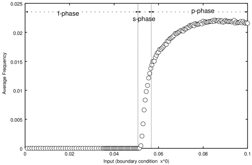
Figure 7: Input dependence of the average frequency of pulses at down-flow is plotted. From the power spectrum, it is shown that the p-phase lies at $x^{0}>0.054$, and s- phase at $0.054>x^{0}>0.051$. For both the phases, the average frequency changes with the input value $x^{0}$. Parameters $a,b,c,d,K,\epsilon$ and intensity of noise $\sigma$ are same as Fig.4.

5 Mechanism

How is the input dependence formed? Recall the following two properties described in §2.2: First, the formation of a pulse train structure depends on if the fixed point solution is CS or CU. Second, the nature of the generated oscillation is influenced by the degree of convective instability of the fixed point at the region where the pulse is being formed.

By referring to these properties, the mechanism of input dependent dynamics is sketched as follows: Depending on the input, the fixed point values at the upper flow change, which leads to the difference in convective instability. Accordingly the degree of the noise amplification changes, and the generated dynamics at the down-flow is different. In this section we study the above mechanism of the input dependence in the term of the convective instability of the fixed point.

Without noise, all elements converge to fixed points $(x^{i}_{*},y^{i}_{*})$ that depend on the site $i$. Now we introduce the site-dependent co-moving Lyapunov exponent $\lambda_{v}(i)$ and spatial instability exponent $\lambda^{S}(i)$ of $(x^{i}_{*},y^{i}_{*})$. We will see that the input dependence can be explained by spatial change of $\lambda^{S}(i)$ for $(x^{i}_{*},y^{i}_{*})$.

5.1 spatial convergence of fixed point

In our model, $(x^{i}_{*},y^{i}_{*})$ is determined as follows.

$$\left\{\begin{array}[]{ll}\dot{x^{i}_{*}}=f(x^{i}_{*},y^{i}_{*},x^{i-1}_{*})&=0\\ \dot{y^{i}_{*}}=g(x^{i}_{*},y^{i}_{*})&=0\end{array}\right.$$ (8)

Eq.(8) gives a recursion equation of from $(x^{i-1}_{*},y^{i-1}_{*})$ to $(x^{i}_{*},y^{i}_{*})$. Given $x^{0}$ at the left boundary, this equation can be solved successively for $i=1,2,....$ by the iteration. The trace of spatial convergence, $(x^{1}_{*},y^{1}_{*})$ $\rightarrow$ $(x^{i}_{*},y^{i}_{*})$ $\rightarrow$ $(x^{\infty}_{*},y^{\infty}_{*})$ is decided as in Fig.8. In our model, $(x^{\infty}_{*},y^{\infty}_{*})$ is decided uniquely to $\forall x^{0}$. We use the notation,

$$\begin{array}[]{rcl}(x_{*},y_{*})&\equiv&(x^{\infty}_{*},y^{\infty}_{*})\\ \lambda^{S}_{*}&\equiv&\lambda^{S}_{*}(\infty)\end{array}$$ (9)

Figure 8: The fixed point $x_{*}(i)$ is plotted for different input values $x^{0}$. Parameters $a,b,c,d,K,\epsilon$ are same as Fig.4. Different marks corresponds to different input values, $x^{0}=0.01(+)$, $0.02(\times)$, $0.03(\bigtriangleup)$, $0.04(\Box)$, $0.05(\bigtriangledown)$, $0.06(\circ)$, and $0.07(\bullet)$.

Now let us study the convective stability of this fixed point. Since the fixed point is site dependent, we extend the co-moving Lyapunov exponent to a spatially local one, by measuring the amplification of perturbation to the next site from each site for a given velocity. Technically this amplification rate is measured as the co-moving Lyapunov exponent for a snapshot homogeneous pattern $(x^{l},y^{l})=(x^{i}_{*},y^{i}_{*})$ for $l\geq i$ (see Appendix).

(a) (b)

Figure 9: Co-moving Lyapunov exponents $\lambda_{v}(i)$ (a) and the spatial instability exponents $\frac{\lambda_{v}(i)}{v}$ (b) are plotted as a function of $v$, for $i=$ $0(\Diamond)$, $5(+)$, $10(\Box)$, $15(\times)$, $20(\bigtriangleup)$, $25(\ast)$, $30(\Diamond)$, $35(+)$, $40(\Box)$. Parameters $a,b,c,d,K,\epsilon$ are same as Fig.4. The boundary condition is given by $x^{0}=0.060$. $\frac{\lambda_{v}(i)}{v}$ is maximum at $v\sim 0.1$ for every site.

Fig.9(a) gives the co-moving Lyapunov exponent $\lambda_{v}(i)$ of the fixed point at each site, while $\frac{\lambda_{v}(i)}{v}$ of the fixed point at each site is given in Fig.9(b). Here, site dependence is clearly seen. At $i\leq 30$ the fixed point is CU, since $\lambda_{v}(i)$ is positive at $v\sim 0.1$. On the other hand, at $i\geq 30$, the fixed point is CS, $\lambda_{v}(i)$ is negative for all $v$. In our model, the fixed points change from convectively unstable to stable ones, as the site goes down-flow.

Recall the growth rate of the perturbation to the next sites is given by the spatial instability, $\lambda^{S}(i)=\mathop{max}_{v}\frac{\lambda_{v}(i)}{v}$. In our model, such velocity $v$ that maximizes $\frac{\lambda_{v}(i)}{v}$ is independent of $i$, as is shown in Fig.9(b). Change of $\lambda^{S}(i)$ with the input $x^{0}$ is shown in Fig.10. In our model, the change is monotonic with respect to site $i$ , either by decreasing from $\lambda^{S}_{*}(1)$ to $\lambda^{S}_{*}$ or increasing.

Now we discuss the relationship between $\lambda^{S}_{*}(i)$ and input dependence. In Table 1, we have classified our dynamics into three types according to the convective stability at the up-flow and down-flow.

Table 1: Composition of CS or CU states at up-flow and down-flow

	fixed point	fixed point	limit cycle
	at up-flow	at down-flow	at down-flow
Type 1	CS	CS	none
Type 2	CU	CS	CS
Type 3	CU or CS	CU	CS

Figure 10: The spatial instability exponent $\lambda^{S}_{*}(i)$ of the fixed point. Different marks represent different input value, $x^{0}=0.01(+)$, $0.02(\times)$, $0.03(\bigtriangleup)$, $0.04(\Box)$, $0.05(\bigtriangledown)$, $0.06(\circ)$, and $0.07(\bullet)$, corresponding to Fig.8.

First, for the Type1, no oscillation is generated, since the fixed point is CS. The fixed point approaches a constant value for $i\rightarrow\infty$, and the state value at the down-flow is input independent. For the Type3 the fixed point at the down-flow is CU, and spatial amplification from a fixed point always occurs, independently of the input value $x^{0}$. Hence, no digital change occurs. Indeed, in numerical simulations, the digital change from a fixed point to oscillation is observed only at the Type2 case only. In this case, there are two CS states at $i\rightarrow\infty$. One is the fixed point $(x_{*},y_{*})$ which is LS (Linearly Stable), and the other is a limit cycle. According to the nature of the up-flow dynamics, either of the two states is selected, that leads to a digital change in the dynamics.

5.2 mechanism of digital change

In this section mechanism of digital change is quantitatively analyzed according to the co- moving Lyapunov exponent.

Since the fixed point becomes convectively stable at the down-flow, the oscillatory dynamics should be formed before the fixed point is stabilized. Hence the condition for the formation of oscillatory dynamics is given by the competition between two time scales, the scale $i_{u}$ where the lattice remains to be CU, and other the scale $i_{g}$, required to the generation of a pulse, i.e. the “growth scale” for perturbation. The scale $i_{u}$ is given by the site where the fixed point $(x^{i}_{*},y^{i}_{*})$ becomes CS, and it is given by the condition $\lambda^{S}(i)>0$ at $i<i_{u}$ and $\lambda^{S}(i)<0$ at $i>i_{u}$.

The scale $i_{g}$ is estimated as the scale where the noise is amplified to the scale of O(1), to generate oscillatory dynamics. As long as the noise is small, the amplification rate of noise is determined by the spatial instability $\lambda^{S}_{*}(i)$ of fixed point $(x^{i}_{*},y^{i}_{*})$. Hence $i_{g}$ is roughly estimated as follows.

$$\sigma\prod^{i_{g}}_{i=0}e^{\lambda^{S}_{*}(i)}=\sigma e^{\sum^{i_{g}}_{i=0}\lambda^{S}_{*}(i)}\sim 1$$ (10)

$$\sum^{i_{g}}_{i=0}\lambda^{S}_{*}(i)\sim log\frac{1}{\sigma}$$ (11)

Since the perturbation is no longer amplified at a CS state, it is necessary that noise is amplified while the dynamics at the site remains to be CU. The noise has to be amplified to O(1) before $i\sim i_{u}$, the condition $i_{g}\stackrel{{\scriptstyle<}}{{\sim}}i_{u}$ is imposed to have oscillatory dynamics. As the input (boundary) changes, fixed points $(x^{i}_{*},y^{i}_{*})$ change accordingly, and both $i_{u}$ and $i_{g}$ change. Then the relation between $i_{g}$ and $i_{u}$ can change qualitatively. Fig.11 shows input dependence of $i_{g}$ and $i_{u}$ for our model for parameters belonging to Type2. Note that the relationship $i_{g}\stackrel{{\scriptstyle>}}{{<}}i_{u}$ changes with the input $x_{0}$. For $x^{0}>0.065$, $i_{g}$ is smaller than $i_{u}$, and indeed we have observed oscillatory dynamics with a large amplitude. Around $x^{0}\sim 0.065$, $i_{g}\sim i_{u}$, where stochastic oscillation is found with intermittent pulse generation from the fixed point state. No pulse is generated for $x^{0}<0.065$.

We can summarize the change of dynamics according to the relationship between $i_{g}$ and $i_{u}$, as follows:

• $i_{g}<i_{u}$ : This gives periodic phase, where stationary oscillation is formed at down-flow. Since the generated oscillation itself is CS, the pulse is transmitted to down-flow without affected by noise. As long as noise is added stationarily (at least at the up-flow), spatially stationary state is formed at the down-flow.

• $i_{g}\sim i_{u}$ : This corresponds to the stochastic phase, where the formation of pulse is strongly sensitive to noise at the moment. Formed pulse itself is CS and can be transmitted to down-flow stationarily, but its formation is intermittent. Indeed, we have measured $\frac{i_{u}}{i_{g}}$ at the parameters of the stochastic phase, and the value stays around $1.0\sim 1.2$.

• $i_{g}=\infty$ ($i_{g}>i_{u}$) : This give a fixed point phase, since the fixed point becomes CS before a pulse is generated. No pulse exists, and the down-flow dynamics remains around the fixed point with some noise. Indeed, the condition(10) is not satisfied for any $i_{g}$.

This summarizes how the digital change appears for our dynamics. It should be noted that the above mechanism generally holds in a one-way coupled system with the fixed points convectively unstable at the up-flow and stable at the down-flow. Now it is also clearer why the digital change is seen only for the Type2. For the Type1, $i_{u}$ is $\infty$, and only the fixed point phase appears, while for the Type3, $i_{u}$ is zero, and the pulse is formed irrespective of the boundary condition (input). The mechanism is shown schematically in Fig.12.

Figure 11: Dependence of $i_{u}$ ($+$) and $i_{g}$ ($\circ$) on input value $x^{0}$. For the reference the change of variance of $x^{80}$ ($\Box$) is plotted. Parameters $a,b,c,d,K,\epsilon$ are same as Fig.4. Intensity of noise $\sigma=0.001$.

Figure 12: Schematic diagram of the change of $\lambda^{S}_{*}$, corresponding to each of the three phases.

5.3 mechanism of analogue change

Here we discuss the analogue change against input, that ’transforms’ the input concentration to the response frequency. The rate of formation of pulse is expected to depend on the fixed points and the convective instability before the pulse train is formed. On the other hand, as the site goes down-flow, the fixed point approaches $(x_{*},y_{*})$ independent of the input $x^{0}$. In other words, the spatial instability is independent of the input, after the fixed point converges closely to $(x_{*},y_{*})$. Hence, only if the scale $i_{g}$, required to form the pulse, is smaller than the scale of the above convergence, the dynamics generated at the down-flow is expected to depend on the input.

As a simple measure of the relaxation length $i_{r}$ of fixed points, we will introduce a ’half-decay’ scale. Since the spatial convergence of $\lambda^{S}_{*}(i)$ is monotonic as described in §5.1 and $\lambda^{S}_{*}(i)$ characterizes the amplification of noise, we use the convergence of $\lambda^{S}_{*}(i)$ to define $i_{r}$. As the half-decay scale of $\lambda^{S}_{*}(i)$, $i_{r}$ is defined such site that satisfies $\lambda^{S}_{*}(i_{r})=\frac{\lambda^{S}_{*}+\lambda^{S}_{*}(0)}{2}$. Roughly speaking, $\sum_{j}^{i}\lambda^{S}_{*}(i)$ changes sensitively on $i$ for $i<i_{r}$, while for $i>i_{r}$, it weakly depends on $i$. This is expected, for example, by assuming that $\lambda^{S}_{*}(i)$ exponentially relaxes to $\lambda^{S}_{*}$.

Now let us focus on the relationship between $i_{g}$ and $i_{r}$. If the convergence scale $i_{r}$ is much smaller than $i_{g}$, the rate of amplification of noise given by $\sum_{j}^{i}\lambda^{S}_{*}(j)$ depends little on the input. On the other hand, if $i_{r}$ is larger than $i_{g}$, the amplification rate largely depends on the input. Since this change of amplification rate is continuous with the input value, analogue change of response is expected. Hence the following two cases are classified.

Case A

: $i_{g}<i_{r}$

At the region where the pulse is formed ($i<i_{g}$), the spatial convergence of fixed points is not yet completed. The noise amplification rate there is dependent on the input. Thus the nature of generated wave at $i\sim i_{g}$ depends on the input. Since the formed wave pattern is convectively stable, this dependence on the input is preserved to down-flow.

Case B

: $i_{g}>i_{r}$

Since the fixed point has almost converged to $(x_{*},y_{*})$ at the site where the wave pattern is formed, the amplification of noise and the nature of formed wave are insensitive to the input value. Hence the nature of generated wave depends little on the input.

To write down the condition for the analogue dependence for the Type2, we need to add the condition for the formation of wave (discussed in §5.2), while for the Type3 the wave is always formed. Hence the conditions of the analogue dependence on the input are summarized as

$$\left\{\begin{array}[]{ll}\mbox{Type2 \ : \ }(i_{g}<i_{r})\cap(i_{g}\stackrel{{\scriptstyle<}}{{\sim}}i_{u})\\ \mbox{Type3 \ : \ }i_{g}<i_{r}\end{array}\right.$$ (12)

In Fig.13 the above mechanism of the analogue change is shown schematically.

(a) (b)

Figure 13: Schematic diagram of the analogue change. Cases with a clear analogue change (a), and without it (b).

Note again that our mechanism for input dependence works universally in one-way coupled dynamical systems, irrespective of the choice of our specific model. In our model, the analogue change is represented as the frequency of oscillations. This transformation of the input to the frequency can be model specific. In general, there may be a variety of ways of transformation of input values to dynamics at the down-flow. Still the argument presented here is applicable to each case.

6 Noise effect to input dependence

In the previous section, the mechanism of input dependence is explained from the spatial change of $\lambda^{S}(i)$. In this section, mechanism of input dependence is discussed from a different angle, that is the relation between convective instability and noise (fluctuation) intensity. It will be shown that the input dependent dynamics at the down-flow is seen only within some range of noise intensity.

Fig.14 shows our numerical results on the input dependence of the variance of $x^{i}(t)$ at the down-flow for different amplitudes of noise, where the parameters are fixed so that the system belongs to Type3. It is seen that the mean square variance has input dependence only in medium intensity ($\bullet$) of the noise. For too large ($\times$) intensity of the noise, the variance does not show input dependence, while the dependence gets weaker as noise amplitude is decreased ($+$). “Suitable” range of noise intensity is required to have analogue change on the input.

Figure 14: Mean square variance $(<(x^{i})^{2}>-<x^{i}>^{2})^{1/2}$ is plotted against the change of input values, for 3 different values of noise amplitudes. $+$ ($\sigma=1.0\times 10^{-7}$) $\rightarrow$$\bullet$ ($\sigma=3.0\times 10^{-3}$) $\rightarrow$$\times$ ($\sigma=8.0\times 10^{-2}$). The parameters corresponds to Type3, $a=2.7,b=10.7,c=4.8,d=9.4,K=0.015,\epsilon=4.5$.

6.1 disappearance of input dependence at a low noise regime

The mechanism of the disappearance of input dependence at a low noise regime is straightforwardly explained with the argument of the previous section. According to eq.(11), $i_{g}$ gets larger with the decrease of the noise, and the relationship between $i_{g}$ and $i_{u}$ or $i_{r}$ changes. With the decrease of $\sigma$, the following two changes are possible.

1. Disappearance of digital change (for Type2):

   With the decrease of $\sigma$ by fixing the input, $i_{g}$ can be larger than $i_{u}$, and the transition from the periodic to stochastic phase, and then to fixed point phase occurs. The periodic phase no longer appears irrespective of the input values (within their allowed range in our model) for small $\sigma$. Hence digital dependence on inputs disappears.

   Fig.15(a) shows input dependence of the variance at the down-flow dynamics with the change of the noise amplitude, while in Fig.15(b) input dependence of $i_{g}$ and $i_{u}$ is plotted. It is demonstrated that the digital change requires larger input values as the noise amplitude is decreased.

   (a) (b)

   Figure 15: Input dependence of the variance at $i=80$ (a)and of $i_{u}$ ($+$) and $i_{g}$ (b) are plotted. The noise amplitudes are $\sigma$ = $10^{-3}(\times)$, $10^{-5}(\circ)$, $10^{-7}(\Box)$, $10^{-9}(\bullet)$ for each figure (Note $i_{u}$ does not depend on $\sigma$). The smaller the noise amplitude is, the harder the periodic phase appears within allowed range of inputs. Parameters $a,b,c,d,K,\epsilon$ are same as in Fig.4.

2. Disappearance of analogue change (for Type2 or Type3):

   With the decrease of $\sigma$, $i_{g}$ increases until it gets larger than $i_{r}$, and the change from CaseA to CaseB in §5.3 follows. Thus analogue dependence on the input fades out.

The lower limit for the noise $\sigma_{S}$ to have the input dependence is straightforwardly estimated from the above argument. The noise intensity must satisfy

$$i_{g}<\left\{\begin{array}[]{ll}i_{r}\mbox{ \ (analogue change)}\\ i_{u}\mbox{ \ (digital change)}\end{array}\right.$$ (13)

By introducing the average spatial instability $\overline{\lambda^{S}_{*}}=(1/i_{g})\sum_{i}^{i_{g}}\lambda^{S}_{*}(i)$, and using the expression eq.(11) for $i_{g}$, we obtain

$$\sigma>\sigma_{S}=\left\{\begin{array}[]{ll}exp(-\overline{\lambda^{S}_{*}}i_{r})\mbox{ \ (analogue change)}\\ exp(-\overline{\lambda^{S}_{*}}i_{u})\mbox{ \ (digital change)}\end{array}\right.$$ (14)

6.2 collapse of input dependence for a strong noise intensity

The collapse of input-dependence at strong noise is due to a different mechanism. When the noise intensity is too large, the wave, once formed, can be destroyed due to the noise at the down-flow. The generated oscillation is distorted by noise and the transmission to down-flow does not work well. In particular, for the Type2 case, due to the convective stability of the fixed point at the down-flow, the dynamics can stay near the fixed point, after the collapse of the limit cycle. Thus, the input dependence between the periodic and fixed point states fades out. There is an upper limit of noise intensity $\sigma_{L}$ such that the input dependence disappears for $\sigma>\sigma_{L}$.

This upper limit $\sigma_{L}$ cannot be estimated by the convective stability of the fixed point. It is a nonlinear effect of noise around the limit cycle oscillation, for which no theory is available as yet.

7 Discussion and conclusions

In the present paper we have reported boundary (input) dependence in a one-way coupled differential equation, and presented a general mechanism for it. It is shown that the spatially dependent convective instability and noise lead to such boundary dependence.

Boundary condition dependence has also been studied in dissipative structure[12]. However our boundary condition dependence is clearly distinguished from earlier studies, and is essential in nature.

The most important difference is dependence on the system size. The boundary condition dependence previously studied is nothing but a finite size effect. The dependence disappears as the size gets larger. On the other hand, our boundary condition dependence is not due to such a finite size effect, but remains even in the infinite size limit. Difference of dynamics, created by the boundary (input) difference, is fixed to the down-flow element $i$ and is kept even for the limit $i\rightarrow\infty$. Also it should be noted that our boundary dependence is independent of initial conditions, and is stable against perturbations.

Furthermore our mechanism supporting the boundary dependence is novel, and should be distinguished from that by the previous studies. In our case, it is originated in the spatial amplification of fluctuation by the convective instability, in contrast with the use of a stable system in the earlier studies [12]. The amplification rate of fluctuation, characterized by the (local) convective Lyapunov exponent $\lambda_{v}(i)$, depends on space, and accordingly on the boundary (input). After the amplification, the dynamics is stabilized at the down-flow. Once stabilized, the dynamics stays as an attractor. Dynamics before the achievement of the spatial convergence can depend on the boundary. On the other hand, the generated difference at the down-flow dynamics cannot be changed any more and is fixed, due to the stable dynamics there. Hence the boundary dependence is fixed at down-flow.

We have shown that there are two types of boundary (input) dependence. One is the threshold-type (bifurcation-like) change, leading to qualitative difference in the down-flow dynamics. In our model, bifurcation from the fixed point, to the stable stochastic oscillation, and then to the stable periodic oscillation is found with the change of the boundary value. The other is continuous (analogue) change of down-flow dynamics, depending on the boundary value. In our example, the frequency of pulses can continuously change with the boundary value.

These two types of boundary dependence are quantitatively analyzed by introducing three characteristic length scales based on the local convective Lyapunov exponent $\lambda_{v}(i)$. The first one is the length scale $i_{g}$ necessary for the fluctuation to be amplified to the macroscopic order. The second is the length scale $i_{u}$ where the convective instability of the fixed point disappears and the dynamics becomes convectively stable. The third is the length scale $i_{r}$ characterizing the spatial convergence of $\lambda_{v}(i)$.

For the bifurcation-like change, it is crucial if the amplification of fluctuation is completed before the fixed point dynamics becomes stable. Otherwise, the down-flow dynamics remains at the fixed point motion. Thus the condition for the qualitative change against the boundary is determined by $i_{g}\stackrel{{\scriptstyle>}}{{<}}i_{u}$. On the other hand, the analogue change depends on if the amplification is completed while the spatial dependence of the convective stability is significant, and thus is judged by the condition $i_{g}\stackrel{{\scriptstyle>}}{{<}}i_{r}$. Note that these conditions also imply that such boundary dependence is seen only within some range of noise amplitude $\sigma$, because $i_{g}\propto log\sigma$ from eq.(11).

Since our mechanism is expressed in universal terms in dynamical systems, the input (boundary) dependence is expected to be observed generally in a spatially extended dynamical system, as long as the spatially inhomogeneous convective instability exists. It is interesting to search for such boundary dependence for open-fluid flow, optical system [3], coupled map lattice[4, 7], and so forth, and to check if the relationship among $i_{g}$ and $i_{u}$ and $i_{r}$ are satisfied.

Our motivation for this study is originated in biological signaling problems. Then what implications are drawn from our result to such problems?

In our study the input information is represented by the boundary value, while the response is given by a state of the down-flow dynamics. At the region $i\stackrel{{\scriptstyle<}}{{\approx}}i_{g}$ required for the wave formation, the input difference is amplified by the convective instability. The information on the dynamics at this region is translated to the response, through the site dependent $\lambda_{v}(i)$. If the conditions among $i_{g}$, $i_{u}$, and $i_{r}$ are satisfied, input information can be translated to output information through the chemical dynamics at the signaling pathway.

Now let us come back to the questions raised in §1. The first question is on the reason for the length and complication of the signaling pathway, to which our results have some implication. According to our mechanism, we need several sites (larger than $i_{g}$ and $i_{u}$) to have input dependence. This number of sites depends on the parameter, but cannot be too small, as long as the dynamics is not too convectively unstable. Hence the pathway must have a sufficient length, to have input dependence. Of course the signal pathway does not consist of a single chain of reaction, but several chains are mutually influenced. Although extension of our study to a multiple chain case remains as a future problem, it is expected that such complication can afford an effectively long chain required for the input dependence.

The second question on the suitable response to inputs is answered by the above translation of the input (boundary) to response (down-flow dynamics) through spatially dependent convective instability $\lambda_{v}(i)$. In particular, the digital (bifurcation- like) dependence provides a response with some input threshold, while the analogue dependence provides the translation from input concentration to response frequency. Both the dependence are essential to neural and sensory responses. It is also interesting to note that our signal transmission mechanism is different from that given by Hodgkin-Huxley equation for neural signal transmission[13].

The third question on the robust signaling mechanism under thermodynamic fluctuation is most clearly answered by our mechanism. Indeed our input dependence works in the presence of noise, or rather the noise amplitude $\sigma$ has to satisfy $\sigma_{L}>\sigma>\sigma_{S}$. Note that the noise is inevitable in a cell system by thermal fluctuation and also due to a relatively small number of signaling molecules. Indeed the number of most signal molecules is around $N\sim 1000$. Thus the noise of the order $1/\sqrt{N}\sim 0.03$ should exist. The condition $\sigma_{L}>\sigma>\sigma_{S}$ for the input dependence may be suggestive in thinking why most cell response works only within some temperature range, and works in a system of small number of (signaling) molecules.

Of course several studies have to be pursued in future, not only as dynamical systems but also for the application of our viewpoint to biological signaling phenomena. The following list is under current investigation.

1. Extension to a case with complex spatial dynamics of $\lambda_{v}(i)$: In our model $\lambda_{v}(i)$ monotonically relaxes to $\lambda_{v}(\infty)$. In general, the relaxation can be oscillatory or have chaotic transient, as is found in a one-way coupled map lattice (OCML)[14]. In such case, complex input dependence may be expected.

2. Extension to a case with a bi-directional or symmetric coupling: Although the present uni-directional coupling case provides a most straightforward example to see the convective instability, such instability also exists in a bi-directional coupling case, and is characterized by the co-moving Lyapunov exponent $\lambda_{v}(i)$ [9]. Indeed some preliminary studies show that the boundary condition dependence of our type also exists in such case.

3. Extension to a system with several CS attractors at $i\rightarrow\infty$. In this case choice of an attractor can depend on inputs. Complicated dependence on input values may exist in a similar manner with fractal or riddled basin structure for a multiple attractor system.

4. Extension to a non-constant input (boundary). If the boundary oscillates in time, for example, this temporal information of the input (boundary) can be translated to response dynamics. Indeed, in a OCML[7], the input oscillation is selectively transmitted to down-flow depending on its period.

5. Extension to a multiple chain system with multiple inputs. In a signaling process in a cell, several pathways exist, which interact with each other. With multiple boundary values (inputs), a new type of boundary dependence can be expected, such as a response depending on combination of several inputs.

acknowledgments

The authors are grateful to T.Yomo, T.Shibata, and I.Tsuda for stimulating discussions. The work is partially supported by Grant-in-Aids for Scientific Research from the Ministry of Education, Science, and Culture of Japan.

Appendix A calculation of local co-moving Lyapunov exponent of the fixed point $(x^{i}_{*},y^{i}_{*})$

Since the fixed points change their value by sites in our model, the conventional method[6] to calculate co-moving Lyapunov exponent has to be extended. To measure the amplification rate of perturbation at one site $i$, we consider a system where $(x^{j},y^{j})=(x^{i}_{*},y^{i}_{*})$ for $j\geq i$ and compute the amplification rate per lattice point. Let us consider the evolution equation,

$$\dot{\vec{z}}^{j}(t)=\vec{h}^{j}(\vec{z}^{j}(t),\vec{z}^{j-1}(t))$$ (15)

with $\vec{h}^{j}(\vec{z}^{j},\vec{z}^{j-1})=(f(\vec{z}^{j},\vec{z}^{j-1}),g(\vec{z}^{j},\vec{z}^{j-1}))$

The displacement follows the equation,

$$\delta\dot{\vec{z}}^{j}(t)=\frac{\partial{\vec{h}}^{j}(\vec{z}^{j},\vec{z}^{j-1})}{\partial{\vec{z}^{j}}}\delta\vec{z}^{j}(t)+\frac{\partial{\vec{h}^{j}(\vec{z}^{j},\vec{z}^{j-1})}}{\partial{\vec{z}^{j-1}}}\delta\vec{z}^{j-1}(t)$$ (16)

We solve the equation for $\vec{z}^{j}=(x^{i}_{*},y^{i}_{*})$ for $j\geq i$ and $\forall t$ with the initial condition $\delta\vec{z}^{j}(0)=\delta_{0,j}\delta$. The solution can be written as

$$\delta\vec{z}^{j}(t)\equiv J^{j}(t)\delta\vec{z}^{0}(0)$$ (17)

where

$$\dot{J}^{j}(t)=\frac{\partial{\vec{h}}^{j}(\vec{z}^{j},\vec{z}^{j-1})}{\partial{\vec{z}^{j}}}J^{j}(t)+\frac{\partial{\vec{h}^{j}(\vec{z}^{j},\vec{z}^{j-1})}}{\partial{\vec{z}^{j-1}}}J^{j-1}(t)$$ (18)

Here, ${J}^{j}(t)$ is a $2\times 2$ matrix, and is obtained by solving eq.(18) under the initial condition $\delta\vec{z}^{j}(0)=\delta_{0,j}\delta$. By defining $e^{\Lambda_{1}^{j}(t)}$ and $e^{\Lambda_{2}^{j}(t)}$ as absolute values of the eigen values of $J^{j}(t)$ ($\Lambda_{1}^{j}(t)\geq\Lambda_{2}^{j}(t)$) we obtain,

$$\lambda_{v}(i)\equiv\lim_{t\rightarrow\infty}\frac{1}{t}\left.\Lambda_{1}^{j}(t)\right|_{j=vt}$$ (19)

References

- [1] B.Alberts, D.Bray, J.Lewis, M.Raff, K.Roberts, and J.D.Watson, Molecular biology of the cell, (1983)
- [2] I.Tsuda and H.Shimizu, “Self-organization of the dynamical channel”, in Complex systems - operational approaches (ed. H.Haken, Springer 1985) 240- 251.
- [3] K.Otsuka and K.Ikeda, “Cooperative dynamics and functions in a collective nonlinear optical element system”, Phys. Rev. A 39 (1989) 5209-5228.
- [4] K.Kaneko, “Spatial Period-doubling in open flow”, Phys Lett. 111 (1985) 321-325.
- [5] I.S.Aranson, A.V.Gaponov-Grekhov and M.I.Ravinovich, “The onset and spatial development of turbulence in flow systems”, Physica D. 33 (1988) 1-20.
- [6] J.P.Crutchfield and K.Kaneko, “Phenomenology of Spatiotemporal Chaos”, in Directions in Chaos (ed. B.L.Hao, World Scientific 1987) 272-353.
- [7] F. H. Willeboordse and K. Kaneko, “Pattern dynamics of a coupled map lattice for open flow”, Physica D. 86 (1995) 428-455.
- [8] R.J.Deissler and K.Kaneko, “Velocity dependent Lyapunov exponent as a measure of chaos for open flows”, Phys Lett. 119A (1987) 397- 402.
- [9] K.Kaneko, “Lyapunov analysis and information flow in coupled map lattice”, Physica D. 23 (1986) 436-447.
- [10] D.Vergni, M.Falcioni, and A.Vulpiani, “Spatial complex behavior in nonchaotic flow systems”, Phys.Rev.E. 56 (1997) 6170-6172.
- [11] R.J.Deissler, “Noise-sustained structure, intermittency, and the Ginzburg-Landau equation”, J.Stat.Phys. 40 (1985) 371-395.
- [12] G.Nicolis and I.Prigogine, Self-organization in nonequilibrium systems (1977) 131-140.
- [13] A.L.Hodgkin and A.F.Huxley, “A quantitative description of membrane current and its application to conduction and excitation in nerve”, J. Physiol. 117 (1952) 500-544.
- [14] K.Fujimoto and K.Kaneko, in preparation.