Deciphering Secure Chaotic Communication

Abstract

A simple technique for decoding an unknown modulated chaotic time-series is presented. We point out that, by fitting a polynomial model to the modulated chaotic signal, the error in the fit gives sufficient information to decode the modulating signal. For analog implementation, a lowpass filter can be used for fitting. This method is simple and easy to implement in hardware.

Indexing terms: chaotic time-series, secure communication (PACS: 05.45).

Secure communication using chaos has received much attention recently. Various methods for modulating and demodulating a chaotic oscillator have been proposed (see [1] and references cited in [2]). There are two ways to hide the modulating signal inside the chaotic carrier signal. One way is to add a small modulating signal to the chaotic carrier signal whose amplitude is much larger. This is called chaotic masking. In this case, power is wasted in the carrier. Another way to encode the modulating signal is to modulate the parameters of the carrier chaotic oscillator. This method has been demonstrated experimentally by many groups[2].

However, it has also been pointed out that secure communication using chaos can be broken ([3],[4]). The first method in [3] is specific to the Lorenz oscillator case. The second method by Short[4] is more general. In this approach by Short, the modulating signal is assumed to be small and the phase-space of the carrier chaotic oscillator is reconstructed from the transmitted time-series using the standard delay embedding techniques ([6], [7]). The chaotic time-series is predicted by noting the flow of nearby trajectories in the embedded phase-space. Then the fourier transform of the difference between the predicted series and the actual transmitted series is taken and a comb filter is applied. This fourier spectrum now reveals the modulating signal. As noted in [5], this technique works well when the modulating signal amplitude is small. If the amplitude of the modulating signal is large, the phase-space structure of the carrier gets greatly altered and it may not be possible to get a good delay embedding of the carrier oscillator dynamics[5].

Another way to unmask the modulating signal is to plot correlation integral[7] of the chaotic time-series as a function of time. This also contains some information about the modulating signal. However, this method requires lot of computation and works only when the modulating waveform is very slowly varying.

In this brief, we point out a much simpler way to extract the modulating signal without using the phase-space information or sophosticated frequency filtering. This method is simple and easy to implement in hardware for real-time decoding and works well when the modulating parameter variation is sufficiently large. This method has been tested for many continous-time chaotic oscillator systems, including the Glass-Mackey equation that generates more complex chaotic waveforms.

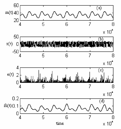
Figure 1: Results for the Lorenz oscillator case. (a) shows the modulating waveform, (b) the transmitted variable $x(t)$, (c) the fit error signal and (d) demodulated output $\hat{m}(t)$.

We take a short segment of the data and fit a polynomial. The number of data points for the fit is kept more than the order of the polynomial. The error in the fit now gives some information about the modulating waveform. As the modulationg parameter is varied, the Lyapunov exponents ($\lambda$’s) of the chaotic oscillator vary and the waveform also varies from, say, a ‘more’ chaotic nature to ‘less’ chaotic nature. When the waveform is less chaotic (smaller positive $\lambda$), we expect the error in the fit to be smaller. The error in the fit becomes larger when the modulating parameter moves the oscillator to a more chaotic region (larger positive $\lambda$).

Since the information about the initial fit is lost within a time interval of about $1/\lambda$, next fit to a nearby segment gives another independent estimate of the fit error. It is easy to get sufficient number of such error points for averaging. The fit error data is then averaged (for about 100-200 points) and applied to a lowpass filter. We used a simple 4th order Butterworth lowpass filter. In case of a single-tone modulating signal, accurate demodulation is easy and a sharp bandpass filter will do. In a more realistic communication system, the baseband modulating signal will consist of a band of frequencies. The results presented here are shown for a two-tone modulating signal of the type $m(t)=A_{1}\sin\omega_{1}t+A_{2}\sin\omega_{2}t$.

We have explored other minor variations of the above technique for calculating the fit error. Some improvement in the demodulated waveform can be found by averging the demodulated signals of different orders of polynomial curve fit. Another way to find the fit error is to project the fitted polynomial to a nearby time location and calculate the fit error in that location. The improvements are only marginal.

First, we show the results for the Lorenz oscillator case with parameters $\sigma=10$, $b=8/3$ and $r=35$ (notations as in [2]). For modulation, the parameter $r$ is varied around its nominal value by the two-tone signal with amplitudes $A_{1}=A_{2}=5$ and $\omega_{1}=2\omega_{2}=0.233$. That is: $r=r_{0}+A_{1}\sin\omega_{1}t+A_{2}\sin\omega_{2}t$. The integration is done using a 4th order Runge-Kutta method with a time step of $\Delta T=0.01$. The variable $x(t)$ of the Lorenz oscillator is assumed to be transmitted. A 4th order polynomial is used to fit every 10 points in the time-series. A 4th order lowpass filter with a small cut-off frequency (0.001/$\Delta T$) is used filter the error signal. The results are summarised in Fig. 1. The demodulated output $\hat{m}(t)$ is shown in Fig. 1d. The fourier frequency spectrum of the error signal (before the final lowpass filter) is shown in Fig. 2. It is clear that the fit error data contains information about the modulating waveform.

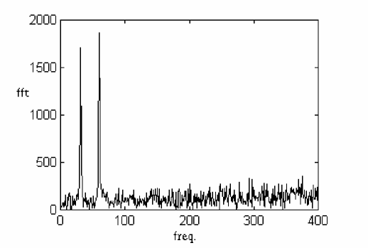
Figure 2: The fourier spectrum of fit error signal $e(t)$.

This demodulation technique requires a digital signal processor (DSP) for real-time decoding. To aviod this, we present another simpler method that can be easily implemented with analog circuitry (Fig. 3). Here, instead of using a DSP or a computer, we use a simple lowpass filter LPF1 (of order 1 or 2) with low time-constant to predict a short segment of the input chaotic time-series. Then the error $e(t)$ between the input signal $x(t)$ and the LPF1 output is calculated. The error can be computed with a squaring or an absolute value circuitry. The delay in the input path can be implemented with a simple I or II order allpass filter. This is to compensate for the delay in LPF1. LPF2 is a sharper lowpass filter (say, of order 4 or 5) with a large time-constant that averages the error signal and produces the output demodulated signal $\hat{m}(t)$. This analog implementation also gives performance comparable to the polynomial fit algorithm given earlier.

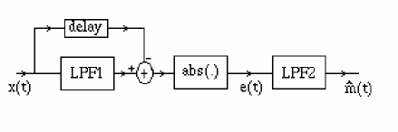
Figure 3: The analog implementation.

The results for the Rossler oscillator case are shown Fig. 4. The Rossler oscillator is simulated with parameters $a=0.2$, $b=0.2$ and $c=5.7$. The $b$ parameter is modulated, as before, with a two-tone modulating signal $A_{1}=A_{2}=0.015$ and $\omega_{1}=2\omega_{2}=0.02$. The time-step for Runge-Kutta method is $\Delta T=0.15$. LPF1 is a 2nd order Butterwoth lowpass filter with a large cut-off frequency ($0.15/\Delta T$). The averaging lowpass filter LPF2 is a 4th order Butterwoth filter with a small cut-off frequency ($0.002/\Delta T$).

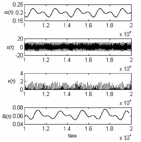
Figure 4: Results for the Rossler oscillator.

Again, the fourier spectrum clearly shows the modulating waveforms. The variation of the output or the $\lambda$’s may not be linear when modulating parameter varies by a large amount. To compensate for this, a non-linear companding/expanding circuitry may be used after demodulation. Thus, it is easy to intercept and decode a continous-time secure chaotic communication.

In conclusion, we have presented a simple algorithm for decoding an unknown modulated chaotic time-series. This technique can be used for real-time decoding using a DSP or an analog circuitry.

References

- [1] K. Cuomo and A. V. Oppenheim, Phys. Rev. Lett. 71, 65 (1993).
- [2] N. J. Corron and D. W. Hahs, IEEE Trans. Circuits. Syst. I 44, 373 (1997).
- [3] G. Perez and H. A. Cerderia, Phys. Rev. Lett. 74, 1970 (1995).
- [4] K. M. Short, Int. J. Bifurc. Chaos 4, 959 (1994).
- [5] L. M. Pecora, T. L. Carroll, G. Johnson and D. Marr, Phys. Rev. E 56, 5090 (1997).
- [6] J. D. Farmer and J. J. Sidorowich, Phys. Rev. Lett. 59, 845 (1987).
- [7] N. B. Abraham . (Eds.), Complexity and Chaos, Nonlinear Science B, vol. 2, 1993, (World Scientific, Singapore).