Quantization of a billiard model for interacting particles

Abstract

We consider a billiard model of a self-bound, interacting three-body system in two spatial dimensions. Numerical studies show that the classical dynamics is chaotic. The corresponding quantum system displays spectral fluctuations that exhibit small deviations from random matrix theory predictions. These can be understood in terms of scarring caused by a 1-parameter family of orbits inside the collinear manifold.

Billiards are interesting and useful models to study the quantum mechanics of classically chaotic systems [3, 4]. In particular, the study of the completely chaotic Sinai billiard [5] and Bunimovich stadium [6] showed that the quantum spectra and wave functions of classically chaotic system exhibit universal properties (e.g. spectral fluctuations) [7] as well as deviations (e.g. scars of periodic orbits) [8] when compared to random matrix theory (RMT) predictions of the Gaussian orthogonal ensemble (GOE) [9].

While the theory of wave function scarring has reached a mature state in two dimensional systems [10, 11, 12, 13] there is a richer structure in more than two dimensions. In particular, invariant manifolds in billiards [14] and systems of identical particles [15] may lead to an enhancement in the amplitude of wave functions [16, 17] provided classical motion is not too unstable in their vicinities.

The purpose of this letter is twofold. First we want to quantize a billiard model for three interacting particles and study a new type of wave function scarring. Second, our numerical results strongly suggest that the system under consideration is chaotic and ergodic. This is interesting in view of recent efforts to construct higher-dimensional chaotic billiards [18, 19, 20].

This letter is organized as follows. First we introduce a billiard model of an interacting three-body system and study its classical dynamics. Second we compute highly excited eigenstates of the corresponding quantum system and compare the results with RMT predictions.

Recently, a self-bound many-body system realized as a billiard has been studied in the framework of nuclear physics [21]. We want to consider the corresponding three-body system with the Hamiltonian

$$H=\sum_{i=1}^{3}{\vec{p}_{i}^{2}\over 2m}+\sum_{i<j}V(|\vec{r}_{i}-\vec{r}_{j}|),$$ (1)

where $\vec{r}_{i}$ is a two–dimensional position vector of the $i$-th particle and $\vec{p}_{i}$ is its conjugate momentum. The two-body potential is

$$V(r)=\left\{\begin{array}[]{ll}0&\mbox{for $r<a$},\\ \infty&\mbox{for $r\geq a$}.\end{array}\right.$$ (4)

The particles thus move freely within a convex billiard in six-dimensional configuration space and undergo elastic reflections at the walls. Besides the energy $E$, the total momentum $\vec{P}$ and angular momentum $L$ are conserved quantities which leaves us with three degrees of freedom. In what follows we consider the case $\vec{P}=0,L=0$.

To study the classical dynamics it is convenient to fix the velocity $\vec{v}_{1}^{2}+\vec{v}_{2}^{2}+\vec{v}_{3}^{2}=1$ and perform computations with the full Hamiltonian (1) without transforming to the subspace $\vec{P}=0,L=0$. We want to compute the Lyapunov exponents of several trajectories. To this purpose we draw initial conditions at random and compute the tangent map [22, 19] while following their time evolution. To ensure good statistics and good convergence we follow an ensemble of $7\times 10^{4}$ trajectories for $10^{5}$ bounces off the boundary. All followed trajectories have positive Lyapunov exponents. The ensemble averaged value of the maximal Lyapunov exponent and its RMS deviation are $\lambda a=0.3933\pm 0.0015$, while the second Lyapunov exponent is also always positive. Thus, the system is chaotic for practical purposes. However, we have no general proof that no stable orbits exist. The reliability of the numerical computation was checked by (i) comparing forward with backward evolution, (ii) observing that energy, total momentum and angular momentum are conserved to high accuracy during the evolution and (iii) using an alternative method [23] to determine the Lyapunov exponent.

The considered billiard possesses two low-dimensional invariant manifolds that correspond to symmetry planes. The first “collinear” manifold is defined by configurations where all three particles move on a line. The dynamics inside this manifold is governed by the one-dimensional analogon of Hamiltonian (1). After separation of the center-of-mass motion one obtains a two-dimensional billiard with the shape of a regular hexagon. This system is known to be pseudo-integrable [24, 25]. To study the motion in the vicinity of the collinear manifold we compute the full phase space stability matrix for several periodic orbits inside the collinear manifold which come in 1-dim families and can be systematically enumerated using the tiling property of the hexagon. All considered types of orbits except two are unstable in the transverse direction: (i) The family of bouncing ball orbits (i.e. two particles bouncing, the third one at rest in between) is marginally stable (parabolic) in full phase space. (ii) The family of orbits depicted in Fig. 1 is stable (elliptic) in two transversal directions and marginally stable (parabolic) in the other 10 directions of 12-dim phase space. Though this behavior does not spoil the ergodicity of the billiard one may expect that it causes the quantum system to display deviations from RMT predictions. Note that this family of periodic orbits differs from the bouncing ball orbits which have been extensively studied in two- and three-dimensional billiards [26, 18] since (i) it is restricted to a lower dimensional invariant manifold, and (ii) it is elliptic (complex unimodular pair of eigenvalues) in one conjugate pair of directions.

The second invariant manifold is defined by those configurations where two particles are mirror images of each other while the third particle is restricted to the motion on the (arbitrarily chosen) symmetry line. Inside this manifold one finds mixed (i.e. partly regular and partly chaotic) dynamics. However, the motion is infinitely unstable in the transverse direction due to non-regularizable three-body collisions.

The quantum mechanics is done using the coordinates

$$\vec{x} = \left(\vec{r_{1}}+\vec{r_{2}}+\vec{r_{3}}\right)/\sqrt{3},$$ (5)

$$\rho\cos{\theta^{\prime}\over 2}\left(\begin{array}[]{c}\cos{(\phi-\varphi^{\prime}/2)}\\ \sin{(\phi-\varphi^{\prime}/2)}\end{array}\right) = \left(\vec{r_{1}}-\vec{r_{2}}\right)/\sqrt{2},$$ (8)

$$\rho\sin{\theta^{\prime}\over 2}\left(\begin{array}[]{c}\cos{(\phi+\varphi^{\prime}/2)}\\ \sin{(\phi+\varphi^{\prime}/2)}\end{array}\right) = \left(\vec{r_{1}}+\vec{r_{2}}-2\vec{r_{3}}\right)/\sqrt{6}.$$ (11)

Here $\rho,\theta^{\prime}$ and $\varphi^{\prime}$ describe the intrinsic motion of the three-body system while $\vec{x}$ and $\phi$ are the center of mass and the global orientation, respectively. In a second transformation we apply a rotation of $\pi/2$ around the abscissa corresponding to spherical coordinates $(\rho,\theta^{\prime},\varphi^{\prime})$, namely $\tan{\varphi}=-\cot{\theta^{\prime}}/\cos{\varphi^{\prime}}$ and $\cos{\theta}=\sin{\theta^{\prime}}\sin{\varphi^{\prime}}$ and obtain for the Laplacian in the subspace $\vec{P}=0,L=0$

$$\Delta={\partial^{2}\over\partial\rho^{2}}+{3\over\rho}{\partial\over\partial\rho}+{4\over\rho^{2}}\left({\partial^{2}\over\partial\theta^{2}}+\cot{\theta}{\partial\over\partial\theta}+{1\over\sin^{2}{\theta}}{\partial^{2}\over\partial\varphi^{2}}\right).$$ (12)

Products of Bessel functions and spherical harmonics

$$\psi_{k,l,l_{z}}(\rho,\theta,\varphi)=(k\rho)^{-1}\,J_{2l+1}(k\rho)\,Y_{l}^{l_{z}}(\theta,\varphi)$$ (13)

are eigenfunctions of the Laplacian (12)

$$\Delta\psi_{k,l,l_{z}}(\rho,\theta,\varphi)=-k^{2}\psi_{k,l,l_{z}}(\rho,\theta,\varphi),$$ (14)

with the usual relation between wavevector and energy $k=\hbar^{-1}(2mE)^{1/2}$. Fig. 2 shows a picture of the billiard taking $(\rho,\theta,\varphi)$ as spherical coordinates. The billiard possesses a $D_{3h}$ symmetry. In the fundamental domain $(\theta,\varphi)\in(0,\pi/2)\times(-\pi/6,\pi/6)$ the boundary is given by

$$\rho_{B}(\theta,\varphi)={a\over\sqrt{1+\sin{\theta}\sin{(\varphi+\pi/3)}}}.$$ (15)

The collinear manifold is the equatorial plane $\theta=\pi/2$. The second invariant manifold is given by the vertical symmetry planes $\phi=\pm\pi/6$. Note that in this representation, classical geodesics of the billiard between two successive collisions are not straight lines since the centrifugal potential is stronger than in Euclidean case. In what follows we restrict ourselves to the fundamental domain and choose basis functions that fulfill Dirichlet boundary conditions. These are bosonic states.

We are interested in highly excited eigenstates. These may be accurately computed numerically by using the scaling method developed in ref. [27] and applied to a three-dimensional billiard by one of the authors [16]. This method works efficiently only when a suitable positive weight function is introduced in a boundary integral. To this purpose we note that the radial part of (12) looks like a 4-dim Laplacian. Extending the results of refs. [27, 16] to four dimensions yields the appropriate weight function, which has a remarkably simple form in our coordinates, namely we minimize the following functional

$$f[\Psi_{k}]=\int_{0}^{1}d\cos\theta\int_{-\pi/6}^{\pi/6}d\varphi\rho_{B}^{4}(\theta,\varphi)|\Psi_{k}(\rho_{B}(\theta,\varphi),\theta,\varphi)|^{2}$$

where the wave-function is expressed in terms scaling functions (13), $\Psi_{k}=\sum_{l}c_{l,l_{z}}\psi_{k,l,l_{z}}$. Due to our particular choice of boundary conditions we consider only the terms for which $l+l_{z}$ is odd and $l_{z}=3m$, and truncate at $l=l_{\rm max}=ka/2+\Delta l\approx ka/2$.

We have computed three stretches of highly excited states. They consist of $7430$, $1813$ and $2362$ consecutive eigenstates with $120<ka<235$, $290<ka<300$ and $393<ka<400$, respectively. The last two stretches comprise levels with sequential quantum numbers around $20000$ and $45000$, respectively. The completeness of the series was checked by comparing the number of obtained eigenstates with the leading order prediction from the Weyl-formula $\bar{d}(k)=c(24\pi^{2})^{-1}(ak)^{2},\;c\approx 0.51349$.

Fig. 3 shows that the nearest neighbor spacing distribution agrees very well with RMT predictions already for the lower energy spectral stretch $120\leq ka\leq 235$. The other series show well agreement, too. As for the long-range spectral correlations, the number variance $\Sigma^{2}(L)$ deviates from RMT predictions for interval length of more than ten mean level spacings which we believe is due to the parabolic-elliptic family of periodic orbits in the collinear manifold (Fig. 1). The deviation from RMT decreases with increasing $k$. For the highest spectral stretch ($ka\approx 400$) the number variance increases linearly, $\Sigma^{2}(L)\approx\Sigma^{2}_{\rm goe}(L)+\varepsilon L$ up to $L\leq 250$, with $\varepsilon\approx 0.04$. This finding is consistent with the model of a statistically independent fraction $\varepsilon$ of strongly scarred states [16]. $\Sigma^{2}(L)$ reaches its maximum and begins to oscillate at the saturation length $L^{*}$ which scales as $L^{*}\propto k^{2}$ in agreement with the prediction of ref. [28].

The length spectrum $D(r)$, i.e. the cosine transform of the oscillatory part of the spectral density $d_{\rm osc}(k)=\sum_{n}\delta(k-k_{n})-\bar{d}(k)$, gives further information about long-range spectral fluctuations. For finite stretches of consecutive levels in the interval $[k_{1},k_{2}]$ one uses a Welsh window function $w(k;k_{1},k_{2})=(k_{2}-k)(k-k_{1})/(6(k_{2}-k_{1})^{3})$ in the actual computation and obtains $D(r)=\int_{k_{1}}^{k_{2}}dk\,w(k;k_{1},k_{2})\cos{(kr)}\,d_{\rm osc}(k)$ (see e.g. [18, 16]). Fig. 4 shows that orbits of length $r=\sqrt{2}a$ and its integer multiples cause dominant peaks in the length spectrum.

To investigate the observed deviations from RMT predictions in more detail it is useful to compute the inverse participation ratio (IPR) of the wave functions in some basis [13]. In the case of billiards the use of the angular momentum basis (13) is particularly convenient and suitable since periodic orbits correspond to sets of isolated points within this representation. Let $c^{(n)}_{l,l_{z}}$ denote the expansion coefficients of $n$th eigenstate $\Psi_{k_{n}}$. We compute the IPR over a set of $N$ consecutive eigenstates as ${\rm IPR}(l,l_{z})=N\sum_{n}|c^{(n)}_{l,l_{z}}|^{4}/(\sum_{n}|c^{(n)}_{l,l_{z}}|^{2})^{2}$. The predicted RMT value for ideally quantum ergodic states is ${\rm IPR}_{\rm goe}=3$. Fig. 5 shows the IPR for the two sets of eigenstates with $170<k<200$ and $290<k<300$, respectively. The agreement with RMT predictions is rather good in both cases. This confirms that the billiard under consideration is dominantly chaotic and ergodic. However, the IPR is slightly enhanced in the region around $l=l_{z}\approx ka/3$. This is a robust phenomenon (present at all energy ranges), although the region of enhancement shrinks with increasing $k$. This finding is compatible with the expectation of uniform quantum ergodicity in the semi-classical limit. Note that the region $l\approx l_{z}$ corresponds to the vicinity of the collinear manifold. Note further that the orbits belonging to the parabolic-elliptic family depicted in Fig. 1 have length $\sqrt{2}a$ and angular momenta in the region $l/ka=l_{z}/ka\in(1/2\sqrt{6},1/\sqrt{6})$. This is precisely the region where the IPR exhibits its enhancement while the orbits’ lengths coincide with the prominent peaks of the length spectrum in Fig. 4.

Thus, the deviations from RMT predictions observed for the spectrum and for the wave functions are associated with the family of parabolic-elliptic periodic orbits inside the collinear manifold. The special stability properties of this family lead to scars in the wave functions of the quantum system. This is an exciting new type of scars of invariant manifolds and complements results previously found in a three-dimensional billiard [16] and in interacting few-body systems [17]. Note that the family of parabolic bouncing ball orbits inside the collinear manifold does not cause statistically detectable scarring. The orbits of this family correspond to points in angular momentum space with $l=l_{z}<ka/2\sqrt{6}$ and do not exhibit an enhancement in the IPR since the classical motion is too unstable in their vicinity.

In summary we have investigated an interacting three-body system realized as a billiard. Numerical results show that the classical dynamics is dominantly chaotic and no deviation from ergodic behavior is found. The spectral fluctuations of the quantum system agree well with random matrix theory predictions on energy scales of a few mean level spacings. However, wave function intensities and long ranged spectral fluctuations display deviations. These can be explained in terms of scars of a family of periodic orbits inside the collinear manifold.

We thank L. Kaplan for stimulating discussions. The hospitality of the Centro Internacional de Ciencias, Cuernavaca, Mexico, is gratefully acknowledged.

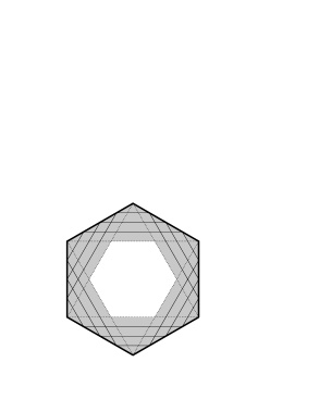
FIG. 1.: The motion inside the collinear manifold corresponds to the motion inside a hexagonal billiard. The parabolic-elliptic family of periodic orbits is shaded. Three of its members and two limiting orbits are presented by full and dotted lines, respectively.

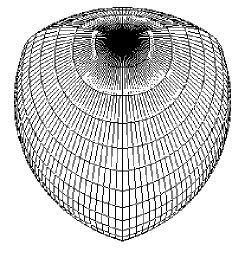
FIG. 2.: Billiard shape after separating off the center of mass motion and rotational degree of freedom.

FIG. 3.: Integrated nearest neighbor spacing distribution $I(S)=\int_{0}^{S}dsP(S)$ with the GOE value subtracted, $I(S)-I_{\rm goe}(S)$, for the set of $N=7430$ consecutive levels with $120<k<235$ (full line). The dashed curve is the estimated statistical error $\sigma=\sqrt{I(S)(1-I(S))/N}$ and the dotted curve is the difference for the commonly used Wigner surmise $I_{\rm wig}(S)=1-\exp(-\pi S^{2}/4)$.

FIG. 4.: Length spectrum $D(r)$ for the long spectral sequence with $120<k<235$. The dashed vertical lines denote the integer multiples of the period of the parabolic-elliptic family.

FIG. 5.: ${\rm IPR}(l,l_{z}=3m)$, for 2052 states with $170<ka<200$ (left) and for 1813 states with $290<ka<300$ (right). Different levels of greyness are used for IPR values on consecutive intervals of width $0.5$. The dominating light-grey corresponds to the interval $[2.75,3.25]$ around the RMT value.

REFERENCES

- [1] address: Institute for Nuclear Theory, Department of Physics, University of Washington, Seattle, WA 98195, USA. e-mail: papenbro@phys.washington.edu
- [2] address: Physics Department, Faculty of Mathematics and Physics, University of Ljubljana, Jadranska 19, 1111 Ljubljana, Slovenia. e-mail: prosen@fiz.uni-lj.si
- [3] O. Bohigas and M.-J. Giannoni, Lecture Notes in Physics Vol. 209 (Springer, Berlin 1984)
- [4] Proceedings of Symposium on Classical and Quantum Billiards, J. Stat. Phys. 83, 1 (1996)
- [5] Y. A. Sinai, Funct Anal. Appl. 2, 61 and 245 (1968)
- [6] L. A. Bunimovich, Funct Anal. Appl. 8, 254 (1974)
- [7] O. Bohigas, M.–J. Giannoni, and C. Schmit, Phys. Rev. Lett.52 1 (1984)
- [8] E. J. Heller, Phys. Rev. Lett.53 1515 (1984)
- [9] T. Guhr, A. Müller-Groeling, and H. A. Weidenmüller, Phys. Rep. 299, 189 (1998)
- [10] E. Bogomolny, Physica D31, 169 (1988)
- [11] M. V. Berry, Proc. R. Soc. Lond. A 423, 219 (1989)
- [12] O. Agam and S. Fishman, Phys. Rev. Lett.73, 806 (1994)
- [13] L. Kaplan, Phys. Rev. Lett.80, 2582 (1998), Nonlinearity 12, R1 (1999)
- [14] T. Prosen, Phys. Lett. A 233, 323 (1997)
- [15] T. Papenbrock and T. H. Seligman, Phys. Lett. A 218, 229 (1996)
- [16] T. Prosen, Phys. Lett. A 233, 332 (1997)
- [17] T. Papenbrock, T. H. Seligman, and H. A. Weidenmüller, Phys. Rev. Lett.80, 3057 (1998)
- [18] H. Primack and U. Smilansky, Phys. Rev. Lett.74, 4831 (1995)
- [19] L. Bunimovich, G. Casati, and I. Guarneri, Phys. Rev. Lett.77, 2914 (1996)
- [20] L. A. Bunimovich and J. Rahacek, Com. Math. Phys. 189, 729 (1997)
- [21] T. Papenbrock, “Collective and chaotic motion in self-bound many-body systems”, preprint DOE/ER/40561-50 (1999)
- [22] M. Sieber and F. Steiner, Physica D44, 248 (1990)
- [23] G. Bennetin, L. Galgani, and J.M. Strelcyn, Phys. Rev. A14, 2338 (1976)
- [24] P. J. Richens and M. V. Berry, Physica D 2 495 (1981)
- [25] B. Eckhardt, J. Ford, and F. Vivaldi, Physica D 13, 339 (1984)
- [26] H.-D. Gräf et al., Phys. Rev. Lett.69, 1296 (1992)
- [27] E. Vergini and M. Saraceno, Phys. Rev. E52, 2204 (1995)
- [28] M.V. Berry, Proc. Roy. Soc. Lond. A400, 229 (1985)