Decomposition of Resonant Scatterers by Surfaces of Section

Abstract

Scattering on the energy shell is viewed here as the relation between the bound states of the Hamiltonian, restricted to sections on leads that are asymptotically independent, far away from the interaction region. The decomposition is achieved by sectioning this region and adding new leads, thus generating two new scatterers. So a resonant scatterer, whose $S$-matrix has sharp energy peaks, can be resolved into a pair of scatterers with smooth energy dependence. The resonant behaviour is concentrated in a spectral determinant obtained from a dissipative section map. The semiclassical limit of this theory coincides with the orbit resummation previously proposed by Georgeot and Prange. A numerical example for a semiseparable scatterer is investigated, revealing the accurate portrayal of the Wigner time delay by the spectral determinant.

I Introduction

Surfaces of section were conceived by Poincaré as a means to decompose bounded classical motion into discrete maps of the section onto itself. Even if the longterm motion is chaotic in some sense, there are many important cases where the single return map is well behaved, so that the complex intermingling of trajectories results from repeated iterations. If a section is badly chosen, the first return map may well be singular and discontinuous with fractal boundaries between continuous regions. Evidently, such a Poincaré map will not be a useful tool for the study of the classical motion. There are many systems for which no single surface exists that leads to a well behaved Poincaré map, though these have not been much studied for obvious reasons.

It is only with the work of Bogomolny [1] that surfaces of section where brought into quantum mechanics. At first this was viewed as an essentially semiclassical extrapolation of Poincaré’s method, while limiting the section to position space instead of the classical phase space. However, the approach of Rouvinez and Smilansky [2] and Prosen [3], allows us to define the transformation, undergone by the finite Hilbert space corresponding to the section, as the product of two unitary scattering matrices. These describe the two alternative unbounded motions, obtained by substituting either side of the system by a semi-infinite tube. Defining the scattering operators as $\mbox{\boldmath$S$}_{L}(E)$ and $\mbox{\boldmath$S$}_{R}(E)$, where $E$ is the energy of the open system, the condition for a bound state to exist at a certain energy is just that $\mbox{\boldmath$S$}_{L}\mbox{\boldmath$S$}_{R}$, or $\mbox{\boldmath$S$}_{R}\mbox{\boldmath$S$}_{L}$ has a unit eigenvalue.

The observation that a “bad” choice of section results in a maze of contributing orbits has a parallel in quantum mechanics that the correponding scattering exhibits multiple resonances. For example, consider the system in Fig. 1(a). For the good choice of section, the classical orbits return to $\Sigma_{A}$ after a short time on the right side, whereas the return map for $\Sigma_{B}$ will be very complex. This corresponds to a smooth energy dependence of all the elements of the scattering matrix $\mbox{\boldmath$S$}_{LA}$ (for the open system obtained by joining an open tube to the left of $\Sigma_{A}$), as opposed to a spiky energy dependence of $\mbox{\boldmath$S$}_{LB}$ due to many resonances. Let us now consider the case where the system under study is actually the open system depicted in Fig. 1(b), obtained by joining a narrow open tube to the left of $\Sigma_{B}$ in system (a). The “natural section” that describes this new scattering problem would then be $\Sigma_{B}$, but having seen that this is a “bad choice” for the closed system, we would also like to bypass it in the description of the new open system (b). It may then be advantageous to decompose this open resonant system using a “good” section $\Sigma_{A}$, just as in the case of the closed system. Indeed, we may consider the latter as the limit of a family of open systems in which the “bad” section is pushed evermore to the left until the opening at $\Sigma_{B}$ has zero width. The system (b) will then be decomposed into the auxiliary systems of Fig. 1(c) and (d). The novelty with respect to the closed problem is that now there are modes entering the scattering region between $\Sigma_{A}$ and $\Sigma_{B}$ from the tubes both to the left and to the right of Fig. 1(c). The important point is that the classical orbits remain only a short time in the scattering region, leading to simple mappings among the surfaces $\Sigma_{A}$ and $\Sigma_{B}$ and nonresonant energy dependence of the $S$-matrices.

The purpose of this paper is to present the general method for the decomposition of a resonant scatterer into two less resonant scatterers by means of a surface of section. If the optimal decomposition renders both the resulting scatterers nonresonant, the objective is reached and the resonances will result from multiple scattering across the surface, as will be explicitly shown in Sec. IV. If there is no choice of section for which one of the components is not resonant, we can clearly decompose it in the same manner and so on until all the components are nonresonant. A similar sequence of decompositions may be required for a bound system. There may not be any surface that avoids resonances in $\mbox{\boldmath$S$}_{L}$ or $\mbox{\boldmath$S$}_{R}$. The further decomposition of either scatterer proceeds exactly as for initially open systems.

First we review multichannel scattering theory on the energy shell, establishing the notation. In Sec. III, we decompose the scatterer through a surface of section. The way that the resonant structure emerges from the decomposed scatterers is described in the following section. Particular attention is given to the time delay, as an overall indicator of resonance. Semiclassical approximations are discussed in Sec. V. These are not valid across a discontinuity, so that the local treatment for its traversal follows in Sec. VI. We conclude with a numerical calculation for a semiseparable scatterer which allows us to evaluate the discontinuous approximation advanced in the previous section. We also verify that the localization of resonance peaks of the time delay is accurately determined by the determinant of a quantum Poincaré map for the open system.

II Multichannel scattering

We here review the theory of scattering on the energy shell so as to define the notation. Careful definition of the context determines the scope of the following theory in its present form. A general scatterer connects regions where asymptotic states, modes or channels, propagate independently. Without loss of generality, we may model the scatterer as a cavity connecting entrance leads[4]. In many important cases, such as in mesoscopic devices, this structure is immediately evident, but even the scattering of waves from a localized object may be considered as radial backscattering along a tube of angular width $2\pi$. Defining $x_{J}$ as the longitudinal coordinate along the $J$-th lead and letting $y_{J}$ represent the transverse coordinates, the asymptotic region is specified by the requirement that, as $x_{J}\to\infty$, the Hamiltonian $H(x_{J},y_{J},p_{xJ},p_{yJ})$ becomes independent of $x_{J}$:

$$H(x_{J},y_{J},p_{xJ},p_{yJ})\stackrel{{\scriptstyle x_{J}\to\infty}}{{\longrightarrow}}\frac{p_{xJ}^{2}}{2m}+H_{J}(y_{J},p_{yJ})\;.$$ (1)

Here we assume that the scattering region lies near the origin of $x_{J}$ and that $x_{J}$ is always positive in the asymptotic region. We also assume bounded motion in the transverse directions, implying that $H_{J}(y_{J},p_{yJ})$ has a discrete infinite spectrum of states $|n_{J}\}$ with energies $\epsilon_{nJ}$.

The Hilbert space for the stationary solutions of the Schrödinger equation are decomposed into orthogonal subspaces in the asymptotic region of each lead. The $J$-th subspace is a superposition of states

$$\langle x_{J},y_{J}|n_{J}\rangle^{\pm}=\frac{1}{\sqrt{k_{nJ}}}\exp(\pm ik_{nJ}x_{J})\{y_{J}|n_{J}\}\equiv\frac{1}{\sqrt{k_{nJ}}}\{y_{J}|n(x_{J})\}^{\pm}\;,$$ (2)

where

$$k_{nJ}=\sqrt{\frac{2m(E-\epsilon_{nJ})}{\hbar^{2}}}\;.$$ (3)

In other words, the interaction between the transverse states $|n_{J}\}$ is switched off as $x_{J}$ enters the asymptotic region. There remains only a trivial exponential dependence of the full state $|n_{J}\rangle$ on the longitudinal coordinate. (We partially adopt the notation of Prosen in [3].)

The states for which $k_{nJ}$ is real are referred to as open channels, otherwise they are closed. For any given energy $E$, there will be a finite number, $\Lambda_{J}$, of open channels. The closed channels with $n_{J}>\Lambda_{J}$ take the form of evanescent modes,

$$\langle x_{J},y_{J}|n_{J}\rangle^{e}=\frac{1}{\sqrt{i|k_{nJ}|}}\exp(-|k_{nJ}|x_{J})\{y_{J}|n_{J}\}\;,$$ (4)

for the wave to be bounded as $x_{J}\to\infty$. However, we shall usually keep to (2) for both open and closed channels.

A general solution $|\psi\rangle$ of the stationary Schrödinger equation is decomposed in the $J$’th tube in terms of transverse amplitudes $\{n_{J}|\psi_{J}\}$

$$\langle x_{J},y_{J}|\psi\rangle=\sum_{n=0}^{\infty}\frac{1}{\sqrt{k_{nJ}}}\left[\{y_{J}|n(x_{J})\}^{+\;+}\{n_{J}|\psi_{J}\}+\{y_{J}|n(x_{J})\}^{-\;-}\{n_{J}|\psi_{J}\}\right]\;.$$ (5)

Here we could also have decomposed $|\psi\rangle$ with the coefficients ${}^{\pm}\{n(x_{J})|\psi\}$ to maintain the symmetry of the bracket notation, but it is easier to use a basis that is independent of $x_{J}$. The incoming wave $|\psi(x_{J})\}^{-}$ and the outgoing wave $|\psi(x_{J})\}^{+}$ at $x_{J}$ are thus defined as

$$|\psi(x_{J})\}^{\pm}\equiv\sum_{n=0}^{\infty}|n(x_{J})\}^{\pm\;\pm}\{n_{J}|\psi_{J}\}\;,$$ (6)

for the open channels. The generalized $S$ matrix is now defined by the equation

$$\left(|\psi(x_{1})\}^{+},|\psi(x_{2})\}^{+},\ldots\right)=\mbox{\boldmath$S$}\left(|\psi(x_{1})\}^{-},|\psi(x_{2})\}^{-},\ldots\right)\;.$$ (7)

Conservation of current among all the leads determines that the restriction of $S$ to the finite block that includes all the open channels is a unitary matrix; time reversal symmetry implies that the full $S$ matrix must be symmetric, i.e., $\mbox{\boldmath$S$}_{ij}$=$\mbox{\boldmath$S$}_{ji}$[2]. Evidently, $S$ depends on the choice of $x_{J}$, but only up to a translation within the asymptotic region, implemented by a diagonal matrix in the $|n(x_{J})\}$ representation. The nontrivial energy dependence of $S$ will be our main concern.

III Decomposition

Let us consider an arbitrary scatterer, with $J$ ($\geq 1$) leads such as sketched in Fig. 2(b). Cutting the scatterer by an arbitrary plane $\Sigma_{0}$, so as to avoid the leads, divides these into $R$-leads to the right of $\Sigma_{0}$ and $L$-leads to the left (either of these sets may be empty). Likewise, we divide all the channels (open and closed) into $R$-channels and $L$-channels. Henceforth it will be immaterial how the independent $R$-channels ($L$-channels) are subdivided among the various $R$-leads ($L$-leads).

Define the coordinate $x_{0}$ growing in the direction normal to $\Sigma_{0}$ and positive on the $R$-side and define the Hamiltonian $H_{0}=H(x_{0}=0)$. Substituting $H$ by $H_{0}$ for all points to the right of $\Sigma_{0}$, we generate a semi-infinite lead. This can be joined onto $H$, to the left of $\Sigma_{0}$ so as to form the $L0$ scatterer sketched in Fig 2(a). This procedure is reflected across $\Sigma_{0}$ to form the $0R$ scatterer, as shown in Fig. 2(c). The $L0$ scatterer has only one $0$-lead on the right and the states $|n_{0}\}$ are the eigenstates of $H_{0}-p_{x_{0}}^{2}/2m$. These coincide with the states to the left of the $0R$ scatterer.

We now derive the relation of the $L0$ and the $0R$ scattering to the original problem, i.e., the $LR$ scattering decomposed by $\Sigma_{0}$. The constant profile of the $H_{0}$ allows us to choose $x_{0}\to 0$ in both the auxiliary scattering problems, which shall be assumed henceforth. The first step is to divide the scattering matrix for each of the scatterers into reflection and transmision blocks, generated by the subdivision of the the channels of each scatterer by $\Sigma_{0}$:

$$\mbox{\boldmath$S$}=\left(\matrix{\mbox{\boldmath$R$}_{LL}&\mbox{\boldmath$T$}_{LR}\cr\mbox{\boldmath$T$}_{RL}&\mbox{\boldmath$R$}_{RR}}\right),~{}\mbox{\boldmath$S$}_{L}=\left(\matrix{\mbox{\boldmath$R$}_{LL}^{0}&\mbox{\boldmath$T$}_{L0}\cr\mbox{\boldmath$T$}_{0L}&\mbox{\boldmath$R$}_{00}^{L}}\right),~{}\mbox{\boldmath$S$}_{R}=\left(\matrix{\mbox{\boldmath$R$}_{RR}^{0}&\mbox{\boldmath$T$}_{R0}\cr\mbox{\boldmath$T$}_{0R}&\mbox{\boldmath$R$}_{00}^{R}}\right)\;.$$ (8)

To avoid confusion, we define the states related by each of these matrices

$$\left(|\psi_{L}(x_{L})\}^{+},|\psi_{R}(x_{R})\}^{+}\right) = \mbox{\boldmath$S$}\left(|\psi_{L}(x_{L})\}^{-},|\psi_{R}(x_{R})\}^{-}\right)\;,$$ (9)

$$\left(|\psi_{L}(x_{L})\}^{+},|\psi_{L0}(x_{0})\}^{+}\right) = \mbox{\boldmath$S$}_{L}\left(|\psi_{L}(x_{L})\}^{-},|\psi_{L0}(x_{0})\}^{-}\right)\;,$$ (10)

$$\left(|\psi_{R}(x_{R})\}^{+},|\psi_{0R}(x_{0})\}^{+}\right) = \mbox{\boldmath$S$}_{R}\left(|\psi_{R}(x_{R})\}^{-},|\psi_{0R}(x_{0})\}^{-}\right)\;,$$ (11)

where $R$, $L$, $0R$, and $L0$ should be taken as specific instances of the index $J$ in the definition (6) and in preceeding formulae. The matrices $S$, $\mbox{\boldmath$S$}_{L}$ and $\mbox{\boldmath$S$}_{R}$ account for the full scattering of three different systems. Our immediate task is to derive the elements of $S$ from those of $\mbox{\boldmath$S$}_{L}$ and $\mbox{\boldmath$S$}_{R}$.

We have already identified the states on the right of the scatterer in Fig. 2(a) with those on the left of Fig. 2(c), as well as those on the left of Fig. 2(a) and (b). Now we match smoothly the wavefunctions of Fig. 2(a) and (c) at $x_{0}=0$. Defining the operators

$$\mbox{\boldmath$k$}_{J}^{\alpha}=\sum_{n}|n\}k_{nJ}^{\alpha}\{n|\;,$$ (12)

for any arbitrary power $\alpha$, we have the matching conditions

$$\mbox{\boldmath$k$}_{0}^{-1/2}|\psi_{L0}(x_{0})\}^{+}+\mbox{\boldmath$k$}_{0}^{-1/2}|\psi_{L0}(x_{0})\}^{-}=\mbox{\boldmath$k$}_{0}^{-1/2}|\psi_{0R}(x_{0})\}^{+}+\mbox{\boldmath$k$}_{0}^{-1/2}|\psi_{0R}(x_{0})\}^{-}$$ (13)

and

$$i\mbox{\boldmath$k$}_{0}^{1/2}|\psi_{L0}(x_{0})\}^{+}-i\mbox{\boldmath$k$}_{0}^{1/2}|\psi_{L0}(x_{0})\}^{-}=-i\mbox{\boldmath$k$}_{0}^{1/2}|\psi_{0R}(x_{0})\}^{+}+i\mbox{\boldmath$k$}_{0}^{1/2}|\psi_{0R}(x_{0})\}^{-}\;,$$ (14)

which determine uniquely

$$|\psi_{0R}(x_{0})\}^{+}=|\psi_{L0}(x_{0})\}^{-}$$ (15)

and

$$|\psi_{L0}(x_{0})\}^{+}=|\psi_{0R}(x_{0})\}^{-}\;.$$ (16)

Inserting these equalities into equations (10) and (11), we obtain

$$\mbox{\boldmath$T$}_{0L}|\psi_{L}(x_{L})\}^{-}+\mbox{\boldmath$R$}_{00}^{L}|\psi_{L0}(x_{0})\}^{-} = |\psi_{0R}(x_{0})\}^{-}\;,$$ (17)

$$\mbox{\boldmath$T$}_{0R}|\psi_{R}(x_{R})\}^{-}+\mbox{\boldmath$R$}_{00}^{R}|\psi_{0R}(x_{0})\}^{-} = |\psi_{L0}(x_{0})\}^{-}\;.$$ (18)

This system of equations for $|\psi_{0R}(x_{0})\}^{-}$ and $|\psi_{L0}(x_{0})\}^{-}$ is easily solved:

$$|\psi_{L0}(x_{0})\}^{-} = \left[\mbox{$\openone$}-\mbox{\boldmath$R$}_{00}^{R}\mbox{\boldmath$R$}_{00}^{L}\right]^{-1}\left[\mbox{\boldmath$R$}_{00}^{R}\mbox{\boldmath$T$}_{0L}|\psi_{L}(x_{L})\}^{-}+\mbox{\boldmath$T$}_{0R}|\psi_{R}(x_{R})\}^{-}\right]\;,$$ (19)

$$|\psi_{0R}(x_{0})\}^{-} = \left[\mbox{$\openone$}-\mbox{\boldmath$R$}_{00}^{L}\mbox{\boldmath$R$}_{00}^{R}\right]^{-1}\left[\mbox{\boldmath$R$}_{00}^{L}\mbox{\boldmath$T$}_{0R}|\psi_{R}(x_{R})\}^{-}+\mbox{\boldmath$T$}_{0L}|\psi_{L}(x_{L})\}^{-}\right]\;,$$ (20)

where $\openone$ is the unit matrix. Combining this result with (10) and (11) again, leads to

$$\mbox{\boldmath$R$}_{LL}^{0}|\psi_{L}(x_{L})\}^{-}+$$ (21)

$$\mbox{\boldmath$T$}_{L0}\left[\mbox{$\openone$}-\mbox{\boldmath$R$}_{00}^{R}\mbox{\boldmath$R$}_{00}^{L}\right]^{-1}\left[\mbox{\boldmath$R$}_{00}^{R}\mbox{\boldmath$T$}_{0L}|\psi_{L}(x_{L})\}^{-}+\mbox{\boldmath$T$}_{0R}|\psi_{R}(x_{R})\}^{-}\right]=|\psi_{L}(x_{L})\}^{+}\;,$$ (22)

$$\mbox{\boldmath$R$}_{RR}^{0}|\psi_{R}(x_{R})\}^{-}+$$ (23)

$$\mbox{\boldmath$T$}_{R0}\left[\mbox{$\openone$}-\mbox{\boldmath$R$}_{00}^{L}\mbox{\boldmath$R$}_{00}^{R}\right]^{-1}\left[\mbox{\boldmath$R$}_{00}^{L}\mbox{\boldmath$T$}_{0R}|\psi_{R}(x_{R})\}^{-}+\mbox{\boldmath$T$}_{0L}|\psi_{L}(x_{L})\}^{-}\right]=|\psi_{R}(x_{R})\}^{+}\;.$$ (24)

But this is just the required linear relation between the incoming waves $|\psi_{L}(x_{L})\}^{-}$, $|\psi_{R}(x_{R})\}^{-}$ and the outgoing waves $|\psi_{L}(x_{L})\}^{+}$, $|\psi_{R}(x_{R})\}^{+}$, so that finally we have

$$\mbox{\boldmath$R$}_{LL} = \mbox{\boldmath$R$}_{LL}^{0}+\mbox{\boldmath$T$}_{L0}\left[\mbox{$\openone$}-\mbox{\boldmath$R$}_{00}^{R}\mbox{\boldmath$R$}_{00}^{L}\right]^{-1}\mbox{\boldmath$R$}_{00}^{R}\mbox{\boldmath$T$}_{0L}\;,$$ (25)

$$\mbox{\boldmath$R$}_{RR} = \mbox{\boldmath$R$}_{RR}^{0}+\mbox{\boldmath$T$}_{R0}\left[\mbox{$\openone$}-\mbox{\boldmath$R$}_{00}^{L}\mbox{\boldmath$R$}_{00}^{R}\right]^{-1}\mbox{\boldmath$R$}_{00}^{L}\mbox{\boldmath$T$}_{0R}\;,$$ (26)

$$\mbox{\boldmath$T$}_{LR} = \mbox{\boldmath$T$}_{L0}\left[\mbox{$\openone$}-\mbox{\boldmath$R$}_{00}^{R}\mbox{\boldmath$R$}_{00}^{L}\right]^{-1}\mbox{\boldmath$T$}_{0R}\;,$$ (27)

$$\mbox{\boldmath$T$}_{RL} = \mbox{\boldmath$T$}_{R0}\left[\mbox{$\openone$}-\mbox{\boldmath$R$}_{00}^{L}\mbox{\boldmath$R$}_{00}^{R}\right]^{-1}\mbox{\boldmath$T$}_{0L}\;.$$ (28)

In this way, the elements of the $S$ matrix for the general scatterer are completely determined by those of the scatterers decomposed by $\Sigma_{0}$.

We now discuss some elementary examples to illustrate the foregoing theory. The most trivial example of a scatterer is an arbitrary section of an open tube. Fixing the surfaces $\Sigma_{R}$ and $\Sigma_{L}$ as in Fig. 3(a), we can “decompose” it with a surface $\Sigma_{0}$ between these. The matrix $\mbox{\boldmath$R$}_{00}=0$, whereas the transmission coefficients are diagonal:

$$\left(\mbox{\boldmath$T$}_{L0}\right)_{nn} = \exp(ik_{n}d_{L0})=\left(\mbox{\boldmath$T$}_{0L}\right)_{nn}^{*}\;,$$ (29)

$$\left(\mbox{\boldmath$T$}_{0R}\right)_{nn} = \exp(ik_{n}d_{0R})=\left(\mbox{\boldmath$T$}_{R0}\right)_{nn}^{*}\;.$$ (30)

A major simplification results in the class of decompositions where there are no tubes on one side of $\Sigma_{0}$, as shown in Fig. 2(b). Then $S$ reduces to

$$\mbox{\boldmath$S$}=\mbox{\boldmath$R$}_{LL}=\mbox{\boldmath$R$}_{LL}^{0}+\mbox{\boldmath$T$}_{L0}\left[\mbox{$\openone$}-\mbox{\boldmath$R$}^{R}_{00}\mbox{\boldmath$R$}^{L}_{00}\right]^{-1}\mbox{\boldmath$R$}^{R}_{00}\mbox{\boldmath$T$}_{0L}\;.$$ (31)

This will be the matrix studied in this Sec. VII, since it already exhibits all the resonant structure of the general case. In the trivial case of a semi-infinite tube, Fig. 2(c), again $\mbox{\boldmath$R$}^{L}_{00}=0$ and $\mbox{\boldmath$T$}_{0L}$ is given by (29), whereas

$$\left(\mbox{\boldmath$R$}^{R}_{00}\right)_{nn}=-\exp(2ik_{n}d_{R})\;,$$ (32)

assuming Dirichlet boundary conditions at the end of the tube.

It is important to remember that the generalized $S$-matrices defined in this section have infinite dimension. Only the blocks made up of all the open channels will be unitary. For this reason, the identification of the open channels for reflection with a unitary $S$-matrix in (31) is only valid because there are no open transmission channels. All projections of a unitary matrix into a subspace define a dissipative matrix with eigenvalues having moduli smaller than one, unless there is no interaction with the subspace that has been projected away[6]. The addition of closed modes does not alter the dissipative nature of the reflection matrices in the general case where transmission is present.

IV Resonance structure: multiple scattering

Let us assume that neither matrix $\mbox{\boldmath$S$}_{R}$ or $\mbox{\boldmath$S$}_{L}$ exhibits a sensitive energy dependence. As previously discussed, such a situation can always be reached in a sequence of decompositions. (Even if the scatterer has a fractal structure, the wavelength settles the smallest scale of the fractal that can be resolved, and thus the number of auxiliary sections will be finite.) The sensitive energy dependence characteristic of a resonant scatterer then emerges from the possibility that one of the eigenvalues of $\mbox{\boldmath$R$}^{R}_{00}\mbox{\boldmath$R$}^{L}_{00}$ or $\mbox{\boldmath$R$}^{L}_{00}\mbox{\boldmath$R$}^{R}_{00}$ approaches the value one. In both cases the spectral determinant

$$\det(\mbox{$\openone$}-\mbox{\boldmath$R$}^{R}_{00}\mbox{\boldmath$R$}^{L}_{00})=\det(\mbox{$\openone$}-\mbox{\boldmath$R$}^{L}_{00}\mbox{\boldmath$R$}^{R}_{00})\to 0\;.$$ (33)

As we show in [6], any block with a smaller dimension than that of a full unitary matrix will generally have eigenvalues with moduli smaller than one. If the channels on the right are closed, $\mbox{\boldmath$R$}^{R}_{00}$ will be unitary, for the channels with real $k_{0}$, but the product with $\mbox{\boldmath$R$}^{L}_{00}$ will still be dissipative. So we never have exactly zero in (33) for scattering situations; indeed these singularities characterize bound states. We may consider the bound states of closed systems as the limit of scattering systems in which the channels both to the right and to the left are closed. The condition (33) is then precisely the well established condition for the existence of an eigenstate [1, 2, 3]. Clearly, the order of the matrices $\mbox{\boldmath$R$}^{L}_{00}$ and $\mbox{\boldmath$R$}^{R}_{00}$ makes no difference to the bound state theory, though it does affect the full scattering problem. For the rest of this section this effect will be unimportant, so we shall abreviate both products $\mbox{\boldmath$R$}^{R}_{00}\mbox{\boldmath$R$}^{L}_{00}$ and $\mbox{\boldmath$R$}^{L}_{00}\mbox{\boldmath$R$}^{R}_{00}$ as simply $\mbox{\boldmath$R$}_{0}$.

The fact that $\mbox{\boldmath$R$}_{0}$ is a dissipative matrix allows us to expand

$$\left(\mbox{$\openone$}-\mbox{\boldmath$R$}_{0}\right)^{-1}=\sum_{\nu=0}^{\infty}\mbox{\boldmath$R$}_{0}^{\nu}\;.$$ (34)

We can thus interpret the formulae for each of the various scattering submatrices as the result of multiple reflections within the resonant region, each one contributing a term to the total scattering matrix. Note that (34) only converges for a scattering system. For a bound system, this is only a formal equality. Therefore, we can regularize the Bogomolny theory for a closed system by considering it as the limit of a scattering system.

The fact that $\mbox{\boldmath$R$}_{0}$ is a well behaved operator with finite trace leads to the Fredholm expansion

$$\left(\mbox{$\openone$}-\mbox{\boldmath$R$}_{0}\right)^{-1}=\frac{1}{D}\sum_{m=0}^{\infty}\sum_{k=0}^{m}D_{k}\mbox{\boldmath$R$}_{0}^{m-k}\;,$$ (35)

where the spectral determinant

$$D\equiv\det\left(\mbox{$\openone$}-\mbox{\boldmath$R$}_{0}\right)=\sum_{m=0}^{\infty}D_{m}\;$$ (36)

and

$$D_{m}=-\frac{1}{m}\sum_{k=1}^{m}D_{m-k}\mbox{Tr}\mbox{\boldmath$R$}_{0}^{k}\;.$$ (37)

This is a similar expansion to that used by Georgeot and Prange [7], but their theory is a reworking of the semiclassical theory, as compared to the exact result. In practice, one must work predominantly with the open channels contemplated by the semiclassical theory (see next section), but this finite matrix can be supplemented by as many closed channels as necessary to obtain convergence.

The main point of the present theory is that we can define a resonant envelope for the energy dependence of all the matrix elements of $S$ as the graph of $D^{-1}(E)$. Certainly, there is a complex coupling among the different transverse states that varies smoothly with energy, so that this graph is not strictly an envelope. Even so, it is only at the peaks of $D^{-1}(E)$ that we will find sharp resonant amplitudes of any element of the $S$ matrix. Not all the peaks of $D^{-1}(E)$ will manifest themselves for a single matrix element, but it is not surprising that collective properties of the $S$-matrix can be much more sensitive to this function of the surface of section. Indeed, the Wigner delay time,

$$\tau(E)=-\frac{i\hbar}{\Lambda}\frac{d}{dE}\log\det\mbox{\boldmath$S$}_{\mbox{{open}}}\;,$$ (38)

where $\Lambda$ is the number of open channels in $S$, measures the globally resonant nature of the scatterer, i.e., the peaks in $\tau(E)$ correspond to the energies of longest permanence in the scattering region for some channel. Near such a peak, we may factor the rapidly varying part of $S$ in (31), or in the more general cases, as

$$\mbox{\boldmath$S$}_{L}\approx D^{-1}(E)\,\mbox{\boldmath$\sigma$}_{L}\;,$$ (39)

where $\mbox{\boldmath$\sigma$}_{L}$ has no peaks. It follows that near the resonant peaks

$$\tau(E)\approx-\frac{i\hbar}{\Lambda}\frac{d}{dE}\log(D^{-\Lambda}\det\mbox{\boldmath$\sigma$})\approx i\frac{d}{dE}\log D\;.$$ (40)

Thus, we obtain the peaks of $\tau(E)\approx\tau_{0}(E)$, where we define the section time delay

$$\tau_{0}(E)=-i\hbar\frac{d}{dE}\log\det(1-\mbox{\boldmath$R$}_{0})^{-1}\;.$$ (41)

We shall verify the validity of this approximate form of the time delay for a numerical example in Sec. VII.

V Semiclassical approximations

The first step towards a semiclassical approximation of the preceeding theory is the truncation of the generalized $S$-matrices, which are restricted to the open channels. The reflections are then described by square sub-matrices, whereas the blocks accounting for transmission will be generally rectangular. Even though all the elements of (25-28) are then well defined, this approximation introduces spurious discontinuities in their energy dependence as each new channel is opened. The semiclassical theory can only avoid these by some form of complex continuation of the classical motion. It should be noted that, even so, the discontinuities in energy do reflect some of the qualitative features of the full quantum theory, so that energy integrals may be quite reasonable. In any case, we expect that truncation will be a good approximation in an energy range with a constant number of open channels, in the limit when this number is large.

We now associate the transverse eigenstates $|n_{J}\}$ singled out by EBK-quantization (see e.g., [8]) on a given section $\Sigma_{J}$ to the invariant tori for the classical Hamiltonian $H_{J}(y_{J},p_{y_{J}})$ defined by (1). In other words, we consider the canonical transformation $(y_{J},p_{y_{J}})$ $\to$ $(I_{J},\theta_{J})$, such that $H_{J}=H_{J}(I_{J})$, obtained from the multivalued generating function $F_{\nu}(I_{J},y_{J})$:

$$\frac{\partial F_{\nu}}{\partial y_{J}}=p_{y_{J}}\;,~{}~{}\frac{\partial F_{\nu}}{\partial I_{J}}=\theta_{J}\;$$ (42)

(where the index $\nu$ distinguishes the different branches). Then we approximate [8]

$$\{y_{J}|n_{J}\}\approx\sum_{\nu}\left|\frac{\partial^{2}F_{\nu}}{\partial I_{J}\partial y_{J}}\right|\exp\left[iF_{\nu}(I_{J},y_{J})/\hbar\right]\;,$$ (43)

with

$$I_{J}(n)=\hbar(n+\mu/4)\;,$$ (44)

where $\mu$ is the Maslov index for the torus. (The phase differences on passing to a different branch are additive, having been included in $F_{\nu}$.) The number of open channels $\Lambda_{J}(E)$ is the largest integer $n$ satisfying the condition

$$H_{J}(I_{J}(n))\leq E\;.$$ (45)

Let us first study scattering where all the points in $\Sigma_{J}$, subject to (45), return to the same region. Semiclassically we have a reflection, $\mbox{\boldmath$S$}=\mbox{\boldmath$R$}$, corresponding to a conservative classical map. Each quantized torus determines a tube of trajectories that re-intersect $\Sigma_{J}$, i.e., it “evolves” while preserving its area as shown in Fig. 4. The overlap of the evolved torus state with the basis of the quantized tori is just

$$\{n^{\prime}_{J}|\mbox{\boldmath$R$}|n_{J}\}\approx\sum_{\nu}\left|\frac{\partial^{2}F_{\nu}}{\partial I_{J}\partial I^{\prime}_{J}}\right|\exp\left[iF_{\nu}(I_{J},I_{J}^{\prime})/\hbar\right]\;,$$ (46)

where the canonical transformation is generated by

$$\frac{\partial F_{\nu}}{\partial I^{\prime}_{J}}=-\theta^{\prime}_{J}\;,~{}~{}\frac{\partial F_{\nu}}{\partial I_{J}}=\theta_{J}\;.$$ (47)

This general formalism for semiclassical maps was originally developed by Miller [5]. The branches, indexed by $\nu$, correspond to each transverse intersection of the new torus with the basis torus $I_{J}=\hbar(n+\mu/4)$. Both the new torus and the basis tori are closed curves (for nonresonant scattering) so there will be an even number of branches. Caustics, leading to spurious singularities in (46), occur when the intersection of the tori is non-transverse, i.e., where two intersections coalesce. In this region the matrix element should be expressed in terms of Airy functions instead of (46) (see e.g., [8]). As we shall discuss below, this simple picture of a returning torus that overlaps with the basis of tori is fragmented into a fractal mosaic for a very resonant system. However, we can now keep to a simple description for each nonresonant scatterer into which the section decomposes the original resonant system.

It is important to note that we need not worry about the problem of quantizing a compact phase space. Our torus basis is infinite, though we are concerned with the projection within a classically invariant region (which grows with $E$). The matrix elements among the open channels in the semiclassical approximation depend only on the classical dynamics within this region. The discrete action variables form a very privileged basis. We cannot transform $R$ to the (semiclassical) $|\theta_{J}\}$ basis without doing a Fourier sum over elements $\{n^{\prime}_{J}|\mbox{\boldmath$R$}|n_{J}\}$ that lie outside the open region, not defined semiclassically. The same difficulty involves passing to the $|y_{J}\}$ representation of $R$. However, the semiclassical evaluation of unitary transformations relies entirely on the stationary phase approximation. We can thus make ordinary semiclassical changes of bases within the allowed region by assuming that there are no stationary phase points outside it.

For scattering where the open channels are not restricted to a single lead, we must consider the conservative classical map defined on the union of several surfaces of section, as shown in Fig. 5. Again, the classical motion takes place on the region (45) for each section, so that the allowed region will vary from section to section. The basis of eigenstates for each section corresponds to a set of quantized invariant tori of that particular section.

To determine the semiclassical approximation to the $S$-matrix when there is more than one lead, we again consider the tube of trajectories defined by one of the quantized tori in one of the sections. But now this tube will generally split, reintersecting the various sections along open segments. Semiclassically, there will be nonzero matrix elements with all the quantized tori with which the segments intersect. The elements of the reflection block are still given by (46), whereas the transmission elements from the $J$-lead to the $K$-lead depend of the generating functions $F_{\nu}(I_{J},I_{K})$ for the canonical transformation $(I_{J},\theta_{J})\to(I_{J},\theta_{J})$ in the form

$$\{n^{\prime}_{K}|\mbox{\boldmath$T$}|n_{J}\}\approx\sum_{\nu}\left|\frac{\partial^{2}F_{\nu}}{\partial I_{J}\partial I_{K}^{\prime}}\right|^{1/2}\exp\left[iF_{\nu}(I_{J},I_{K}^{\prime})/\hbar\right]\;.$$ (48)

By adopting fixed action-angle variables along $\Sigma_{J}$, with the normal coordinate $x_{J}$, the action for orbits returning to the same lead,

$$F_{\nu}(I_{J},I_{J}^{\prime})=\int_{I_{J}}^{I_{J}^{\prime}}\theta_{J}dI_{J}+\oint p_{x_{J}}dx_{J}\;,$$ (49)

except for Maslov indices, is evaluated along the classical orbit joining the torus $I_{J}$ to $I_{J}^{\prime}$. This can also be obtained by taking

$$F_{\nu}(y_{J},y_{J}^{\prime})=\int p_{y_{J}}dy_{J}+\oint p_{x_{J}}dx_{J}$$ (50)

and then evaluating the change of basis by stationary phase. To evaluate the transmission actions, we first note that the difference between (46) and (48) is only that $I_{J}$ and $I_{K}^{\prime}$ belong to different torus bases, rather than they belong to different sections. Defining $F^{0}$ as the generating function for the canonical transformation corresponding to this change of basis we obtain

$$F_{\nu}(I_{J},I_{K}^{\prime})=F_{\nu}^{0}(I_{J},I_{K}^{\prime})+\int_{I_{K}(I_{J})}^{I_{K}^{\prime}}\theta_{K}dI_{K}+\int_{\Sigma_{J}}^{\Sigma_{K}}p_{x}dx\;,$$ (51)

where

$$\frac{\partial F_{\nu}^{0}}{\partial I_{K}^{\prime}}=-\theta^{\prime}_{K}$$ (52)

describes the original torus with action variable $I_{J}$ in the $(I_{K},\theta_{K})$ coordinates; $I_{K}(I_{J})$ is the action variable of the orbit on this torus that will arrive at $I_{K}^{\prime}$ and the variable $x$ in the last integral is assumed normal to both sections.

So far, this review of semiclassical scattering theory applies to an arbitrary scatterer. The problem arises, for a very resonant scatterer that the classical map fragments into arbitrarily small regions which cannot be quantized when their area is smaller that Planck’s constant [6]. However, we have seen that it is always possible to decompose a resonant scatterer by appropriate surfaces of section. It is then possible to adopt semiclassical approximations for each of the components and then to evaluate the blocks of the full $S$ matrix given by (25-28) in the stationary phase approximation.

For a typical resonant scatterer, cut by a “good” section, $\Sigma_{0}$, the classically allowed area in $\Sigma_{0}$ will be considerably larger than the union of the $R$-leads and of the $L$-leads projected onto $\Sigma_{0}$. The classical map corresponding to the various $T$ blocks of the component scatterers will be a simple injection of orbits into $\Sigma_{0}$, or its time reverse. If we decouple this part of the $S$ matrix, there results the view of semiclassical scattering as essentially that of the $\Sigma_{0}$ surface onto itself with projections onto entrance and exit regions, as previously proposed [6]. The semiclassical neglect of any backscattering in the $L0$ or $R0$ scattering depends on the smoothness of the Hamiltonian. It is certainly inadequate for a discontinuity in the Hamiltonian within the range of the longitudinal wavelength. This case will be treated in Sec. VI.

If we apply the Fredholm theory in Sec. III to $[1-\mbox{\boldmath$R$}^{R}_{00}\mbox{\boldmath$R$}^{L}_{00}]^{-1}$ and to $[1-\mbox{\boldmath$R$}^{L}_{00}\mbox{\boldmath$R$}^{R}_{00}]^{-1}$ and then use the semiclassical expressions for each of the reflection matrices, we succeed in rederiving the scattering theory of Georgeot and Prange [7] from first principles. This is especially valuable, because it was originally obtained by the rearrangement of the semiclassical contributions to the scattering matrix, which is not valid in the resonant context. The spectral determinant (36) will be described by the classical periodic orbits that cross the surface $\Sigma_{0}$ rearranged into composite orbits or pseudo-orbits. As we have seen, the spectral determinant is never zero, because the $R$ matrices are dissipative. No matter how long lived the typical classical orbits may be, as counted by the number of traversals of $\Sigma_{0}$, there will be a cuttoff for the period of the periodic orbits included in the Fredholm theory. This is limited to the dimension of the $R$ matrices.

To conclude this section, we note that in the important case of systems with hard walls, i.e., open billiards connected by leads as in Fig. 6, the quantized tori for any section, central to the foregoing theory, will be defined as the level curves of $p_{y}^{2}$. The phase change between the two branches of $\{y|n\}$ will depend upon the choice of Dirichlet or Neumann boundary conditions. It may well be advantageous to use the perimeter of the closed billiard ($\Sigma_{B}$ in Fig. 6), corresponding to the classical Birkhoff map (or bounce map) instead of a section such as $\Sigma_{0}$. This was the point of view adopted in [6]. In this case, all scattering will be considered as a reflection across $\Sigma_{B}$. However, in this case, it is essential to take into account the discontinuity on entering the billiard, which is the subject of the next section.

VI Discontinuities

If the Hamiltonian is discontinuous across a given plane $\Sigma$, we should construct two sections $\Sigma_{L}$ and $\Sigma_{R}$ immediately on either side of $\Sigma$, as shown in Fig. 7. This is an important example of a scattering system which is clarified by the use of extra surfaces of section. In the following theory we only address the local problem of scattering from $\Sigma_{L}$ to $\Sigma_{R}$. With respect to Fig. 7, we may consider the $l\to R$ scattering as decomposed by $\Sigma_{L}$, or that $\Sigma_{R}$ decomposes the $L\to r$ scattering. Thus the full $l\to r$ scatterer will be decomposed in two stages. In the simple semiseparable example discussed in Sec. VII, both the $l\leftrightarrow L$ and $R\leftrightarrow r$ propagators are trivial.

To solve the scattering problem across the discontinuity between the sections $\Sigma_{L}$ and $\Sigma_{R}$ involves the same smoothness conditions as (13) and (14), except that now the wave vectors $\mbox{\boldmath$k$}_{R}\neq\mbox{\boldmath$k$}_{L}$ and we have different basis states $|n_{R}\}$ and $|n_{L}\}$ to match on either side. Recalling the definiton of the operators $\mbox{\boldmath$k$}_{J}^{\alpha}$ in (12), we have

$$\mbox{\boldmath$k$}_{L}^{-1/2}\left[|\psi_{L}\}^{+}+|\psi_{L}\}^{-}\right] = \mbox{\boldmath$k$}_{R}^{-1/2}\left[|\psi_{R}\}^{+}+|\psi_{R}\}^{-}\right]\;,$$ (53)

$$i\mbox{\boldmath$k$}_{L}^{1/2}\left[|\psi_{L}\}^{+}-|\psi_{L}\}^{-}\right] = i\mbox{\boldmath$k$}_{R}^{1/2}\left[-|\psi_{R}\}^{+}+|\psi_{R}\}^{-}\right]\;.$$ (54)

Decomposing the $S$ matrix into reflexion and transmission blocks (8), then yields

$$\mbox{\boldmath$k$}_{L}^{-1/2}\left[(\mbox{$\openone$}+\mbox{\boldmath$R$}_{LL})|\psi_{L}\}^{-}+\mbox{\boldmath$T$}_{LR}|\psi_{R}\}^{-}\right] = \mbox{\boldmath$k$}_{R}^{-1/2}\left[(\mbox{$\openone$}+\mbox{\boldmath$R$}_{RR})|\psi_{R}\}^{-}+\mbox{\boldmath$T$}_{RL}|\psi_{L}\}^{-}\right]\;,$$ (55)

$$\mbox{\boldmath$k$}_{L}^{1/2}\left[(\mbox{$\openone$}-\mbox{\boldmath$R$}_{LL})|\psi_{L}\}^{-}-\mbox{\boldmath$T$}_{LR}|\psi_{R}\}^{-}\right] = \mbox{\boldmath$k$}_{R}^{1/2}\left[(-\mbox{$\openone$}+\mbox{\boldmath$R$}_{RR})|\psi_{R}\}^{-}+\mbox{\boldmath$T$}_{RL}|\psi_{L}\}^{-}\right]\;.$$ (56)

The fact that these equations are valid for any $|\psi_{R}\}^{-}$ or $|\psi_{L}\}^{-}$ allows us to equate separately the operators acting on either of these functions. However, to derive matrix equations, we must transform between the natural bases on either side. Thus, defining the orthogonal matrix

$$\mbox{\boldmath$U$}_{n^{\prime}n}=\{n^{\prime}_{L}|n_{R}\}=\int dy\{n^{\prime}_{L}|y\}\{y|n_{R}\}\;,$$ (57)

we obtain

$$\mbox{\boldmath$k$}_{L}^{-1/2}(\mbox{$\openone$}+\mbox{\boldmath$R$}_{LL}) = \mbox{\boldmath$U$}\mbox{\boldmath$k$}_{R}^{-1/2}\mbox{\boldmath$T$}_{RL}\;,$$ (58)

$$\mbox{\boldmath$k$}_{L}^{1/2}(\mbox{$\openone$}-\mbox{\boldmath$R$}_{LL}) = \mbox{\boldmath$U$}\mbox{\boldmath$k$}_{R}^{1/2}\mbox{\boldmath$T$}_{RL}\;;$$ (59)

where the matrix $\mbox{\boldmath$R$}_{LL}$ is in the $L$-representation, whereas $(\mbox{\boldmath$T$}_{RL})_{nn^{\prime}}=\{n_{R}|\mbox{\boldmath$T$}_{RL}|n_{L}^{\prime}\}$. Alternatively, we obtain from (56) and the transpose of (57) that

$$\mbox{\boldmath$k$}_{R}^{-1/2}(\mbox{$\openone$}+\mbox{\boldmath$R$}_{RR}) = \mbox{\boldmath$U$}^{T}\mbox{\boldmath$k$}_{L}^{-1/2}\mbox{\boldmath$T$}_{LR}\;,$$ (60)

$$\mbox{\boldmath$k$}_{R}^{1/2}(\mbox{$\openone$}-\mbox{\boldmath$R$}_{RR}) = \mbox{\boldmath$U$}^{T}\mbox{\boldmath$k$}_{L}^{1/2}\mbox{\boldmath$T$}_{LR}\;,$$ (61)

where, again, the indices $L$,$R$ specify the bases. Notice that the set of equations (60,61) (and its solution) is related to the set (58,59) by interchanging $L,\mbox{\boldmath$U$}\leftrightarrow R,\mbox{\boldmath$U$}^{T}$(time reversal). So we restrict ourselves to (60,61), which can be solved for

$$\mbox{\boldmath$T$}_{LR} = 2\left(\mbox{\boldmath$k$}_{R}^{1/2}\mbox{\boldmath$U$}^{T}\mbox{\boldmath$k$}_{L}^{-1/2}+\mbox{\boldmath$k$}_{R}^{-1/2}\mbox{\boldmath$U$}^{T}\mbox{\boldmath$k$}_{L}^{1/2}\right)^{-1}\;,$$ (62)

$$\mbox{\boldmath$R$}_{RR} = {\textstyle\frac{1}{2}}\left(\mbox{\boldmath$k$}_{R}^{1/2}\mbox{\boldmath$U$}^{T}\mbox{\boldmath$k$}_{L}^{-1/2}-\mbox{\boldmath$k$}_{R}^{-1/2}\mbox{\boldmath$U$}^{T}\mbox{\boldmath$k$}_{L}^{1/2}\right)\mbox{\boldmath$T$}_{LR}\;;$$ (63)

with $\mbox{\boldmath$T$}_{RL}$ and $\mbox{\boldmath$R$}_{LL}$ given by time-reversal as we previously noted:

$$\mbox{\boldmath$T$}_{RL} = 2\left(\mbox{\boldmath$k$}_{L}^{1/2}\mbox{\boldmath$U$}\mbox{\boldmath$k$}_{R}^{-1/2}+\mbox{\boldmath$k$}_{L}^{-1/2}\mbox{\boldmath$U$}\mbox{\boldmath$k$}_{R}^{1/2}\right)^{-1}\;,$$ (64)

$$\mbox{\boldmath$R$}_{LL} = {\textstyle\frac{1}{2}}\left(\mbox{\boldmath$k$}_{L}^{1/2}\mbox{\boldmath$U$}\mbox{\boldmath$k$}_{R}^{-1/2}-\mbox{\boldmath$k$}_{L}^{-1/2}\mbox{\boldmath$U$}\mbox{\boldmath$k$}_{R}^{1/2}\right)\mbox{\boldmath$T$}_{RL}\;.$$ (65)

It is straightforward to verify that the $S$ matrix for the discontinuity is symmetric. The verification of unitarity is also simple, but lengthy[9].

The matrix inversions in the preceding formulae will be calculated by truncating the bases on the right and on the left of the discontinuity. A possible choice is to limit $U$ to the open channels on either side, but their numbers may not be the same. A better alternative is to notice that the matrix elements $\mbox{\boldmath$U$}_{n^{\prime}n}$ decay exponentially when there is no intersection between the quantized tori corresponding to $|n_{L}\}$ and to $|n^{\prime}_{R}\}$. Therefore, the open channels should be supplemented with states which intersect with them on either side of the discontinuity.

It is interesting that the preceeding argument relies on a semiclassical criterion of torus overlap to calculate $\mbox{\boldmath$U$}_{n^{\prime}n}=\{n^{\prime}_{L}|n_{R}\}$, even though we use this to calculate classically forbidden reflections. We shall use a similar semiclassical approach to estimate the channels exhibiting resonances in Sec. VII. This semiclassical inspiration will now be pushed further to suggest an approximation that avoids the matrix inversions in $S$. To this end, we notice that the semiclassical evaluation of the nondecaying $\mbox{\boldmath$U$}_{n^{\prime}n}$ depends on the points of intersection for the corresponding tori (such as shown in Fig. 10). We could then view each intersection as the projection of an orbit transmitted or reflected at the discontinuity. Thus each orbit contributing to a given matrix element faces the same discontinuity in the longitudinal Hamiltonian, as depicted in Fig. 8. What is the probability amplitude for a wave $|n_{R}\}$ incident on the right to propagate to the left channel $|n^{\prime}_{L}\}$? Separating out the longitudinal motion, we have

$$|x,y_{R}\rangle = \left[k_{nR}^{-1/2}\exp(-ik_{nR}x)+(\mbox{\boldmath$r$}_{RR})_{n^{\prime}n}k_{nR}^{-1/2}\exp(ik_{nR}x)\right]\{y|n_{R}\}\;,x\geq 0\;,$$ (66)

$$|x,y_{L}\rangle = \left[(\mbox{\boldmath$t$}_{LR})_{n^{\prime}n}k_{n^{\prime}L}^{-1/2}\exp(-ik_{n^{\prime}L}x)\right]\{y|n^{\prime}_{L}\}\;,x\leq 0\;.$$ (67)

Here, $\mbox{\boldmath$t$}_{LR}$ and $\mbox{\boldmath$r$}_{RR}$ are the “longitudinal” transmission and reflection matrices. By requiring that both waves match at the discontinuity at $x=0$ we obtain:

$$(\mbox{\boldmath$t$}_{LR})_{n^{\prime}n} = 2\left(\sqrt{\frac{k_{nR}}{k_{n^{\prime}L}}}+\sqrt{\frac{k_{n^{\prime}L}}{k_{nR}}}\right)^{-1}\;,$$ (68)

$$(\mbox{\boldmath$r$}_{RR})_{n^{\prime}n} = \left(\sqrt{\frac{k_{nR}}{k_{n^{\prime}L}}}-\sqrt{\frac{k_{n^{\prime}L}}{k_{nR}}}\right)\left(\sqrt{\frac{k_{nR}}{k_{n^{\prime}L}}}+\sqrt{\frac{k_{n^{\prime}L}}{k_{nR}}}\right)^{-1}\;,$$ (69)

which are the well known results for the one-dimensional step potential. In the case of a two-dimensional discontinuity we still have to take into account the coupling $U_{n^{\prime}n}$ between transverse modes at each side of the discontinuity. The expression for the approximate transmission matrix $\widetilde{\mbox{\boldmath$T$}}$ is thus

$$(\widetilde{\mbox{\boldmath$T$}}_{LR})_{n^{\prime}n}=(\mbox{\boldmath$t$}_{LR})_{n^{\prime}n}\mbox{\boldmath$U$}_{n^{\prime}n}\equiv\left[\mbox{\boldmath$t$}_{LR}\mbox{\boldmath$U$}\right]_{n^{\prime}n}\;.$$ (70)

Similarly $(\mbox{\boldmath$r$}_{RR})_{n^{\prime}n}\mbox{\boldmath$U$}_{n^{\prime}n}$ gives the probability amplitude for not being transmitted to channel $n^{\prime}$. As this probability is distributed over the $L$ basis we must switch back to the $R$ representation. Our approximate result for the reflection matrix reads

$$\widetilde{\mbox{\boldmath$R$}}_{RR}=\mbox{\boldmath$U$}^{T}\left[\mbox{\boldmath$r$}_{RR}\mbox{\boldmath$U$}\right]\;.$$ (71)

The corresponding approximation for the transmission and reflection matrices for waves inciding from the left are obtained by the time reversal operation:

$$\widetilde{\mbox{\boldmath$T$}}_{RL} = \left[\mbox{\boldmath$t$}_{RL}\mbox{\boldmath$U$}^{T}\right]\;,$$ (72)

$$\widetilde{\mbox{\boldmath$R$}}_{LL} = \mbox{\boldmath$U$}\left[\mbox{\boldmath$r$}_{LL}\mbox{\boldmath$U$}^{T}\right]\;.$$ (73)

We can clarify the nature of this two dimensional version of a “sudden approximation” (70) by noting that

$$\mbox{\boldmath$k$}_{L}^{-1/2}\widetilde{\mbox{\boldmath$T$}}\mbox{\boldmath$k$}_{R}^{1/2}\mbox{\boldmath$U$}^{T}+\mbox{\boldmath$k$}_{L}^{1/2}\widetilde{\mbox{\boldmath$T$}}\mbox{\boldmath$k$}_{R}^{-1/2}\mbox{\boldmath$U$}^{T}=2\;$$ (74)

as compared to (62), so that $\widetilde{\mbox{\boldmath$T$}}$ amounts to a reordering of the operators that define $T$. This allows the simplification of not having to invert the matrices in the exact formula (62).

VII A semiseparable numerical example

We now study a simple though nontrivial example of the decomposition of a resonant scatterer. This is chosen as the semiseparable system sketched in Fig.9, i.e., the potential $V(x,y)$ is separable for $x>0$ and for $x<0$, but discontinuous at $x=0$:

$$V(x,y)=\left\{\matrix{\mbox{${\textstyle\frac{1}{2}}$}\omega_{L}^{2}y^{2}&x<0\cr\mbox{${\textstyle\frac{1}{2}}$}\omega_{R}^{2}y^{2}&0<x<a\cr\infty&x=a}\right.\;.~{}$$ (75)

We choose $\omega_{L}>\omega_{R}$, so that the classical motion is broader on the right than on the left: the outline in Fig. 9 represents an equipotential curve. (The main difference with respect to the system studied by Prosen[3] is that it is open in the left.) Computations were carried out with the values $\omega_{L}$=1, $\omega_{R}$=0.71423, $a$=30, $\hbar$=1, and mass $m$=1 (in appropriate units).

Separability on the left allows us to bring the entrance section $\Sigma_{L}$ to $x=0^{-}$. The position of the Poincaré section is also arbitrary, because of separability, so we bring $\Sigma_{0}$ to $x=0^{+}$. There being a single open lead, the decomposition of the scattering matrix is given by (31), where the reflection matrix on the right of $\Sigma_{0}$ is diagonal, with elements

$$\left\{n_{R}|\mbox{\boldmath$R$}^{R}_{00}|n_{R}\right\}=-\exp(2ik_{Rn}a)\;.$$ (76)

The transmission matrices $\mbox{\boldmath$T$}_{L0}$ and $\mbox{\boldmath$T$}_{0L}$ are just those for the passage through a discontinuity of the potential discussed in the last section. This permits us to evaluate the accuracy of the approximation proposed there within the resonant theory. The reflection $\mbox{\boldmath$R$}^{R}_{00}$ may also be calculated in this approximation. In spite of its motivation in terms of classical orbits, one should notice that this “sudden approximation” mixes the motion that fails to escape before it is propagated diagonally by $\mbox{\boldmath$R$}^{R}_{00}$. Thus, the full Poincaré reflection matrix $\mbox{\boldmath$R$}^{R}_{00}\mbox{\boldmath$R$}^{L}_{00}$ is not diagonal, in contrast to the classical motion which is integrable until it escapes.

The $S$ matrix was calculated in an energy range corresponding to 15 open channels, but excluding an interval of 0.2 near the thresholds of the 15th and 16th channels. Evidently each channel threshold is given by

$$E_{n}=\hbar\omega_{L}(n-\mbox{${\textstyle\frac{1}{2}}$})\;.$$ (77)

The number of transverse states on the right corresponding to open channels grows from 21 to 22 in the energy window, with our choice of the frequency $\omega_{R}$.

We can predict which entrance channels may exhibit resonance behaviour by reverting to the qualitative semiclassical picture of Sec. V, even though the discontinuity prevents an accurate semiclassical calculation. The modes in the open lead correspond to the concentric circles of in Fig. 10 with area $2\pi(n_{L}-\mbox{${\textstyle\frac{1}{2}}$})$, whereas the states in the cavity correspond to the ellipses with area $2\pi(n_{R}-\mbox{${\textstyle\frac{1}{2}}$})$ and semiaxes with the ratio $\omega_{R}$. Semiclassically, an incoming mode only excites the inner states corresponding to ellipses that intersects its circle. If these ellipses, in their turn, only intersect circles with $n_{L}\leq 15$, there should be straight nonresonant backscattering for this mode. It is easy to see that, by this criterion, it is only for $n_{L}>15\omega_{R}^{2}\approx 7$ that the resonant structures should arise.

In Fig.11 we compose $D=\det[1-\mbox{\boldmath$R$}^{R}_{00}\mbox{\boldmath$R$}^{L}_{00}]$ and the section time delay with Wigner’s time delay. It is impressive how the overall structure of this global imprint of the resonances is re-composed from both nonresonant matrices $\mbox{\boldmath$R$}^{R}_{00}$ and $\mbox{\boldmath$R$}^{L}_{00}$. It is important to note that the peaks in the time delay are only poorly correlated to the bound states of the separable system obtained by closing the lead at $x=0$, also shown in Fig. 10. [A comment about this plot is in order. Recalling that in (41) we had discarded the slowly varying part of the time delay, we shifted $\tau_{0}(E)$ by a fixed amount so that both average times $\langle\tau_{0}\rangle$ and $\langle\tau\rangle$ coincide. Then logarithms were taken and, finally, the curves corresponding to $\tau_{0}(E)$ and $D(E)$ were shifted downwards to make comparisons easier.]

In Fig.12 we show the resonance structure of individual $S$ matrix elements. Evidently, each one of these does not exhibit all the resonance peaks in the time delay, but the determinant $D$ does limit the positions allowed for these peaks in all cases. We find that the positions of the resonances are reasonably obtained, except for very fine structures, but the amplitudes of the individual matrix elements are not predicted by the spectral determinant. In these figures we also compare the sudden approximation with the exact calculation. This approximation works remarkably well for both nonresonant and resonant channels up to $i$=13.

VIII Concluding remarks

The spiky energy dependence of the $S$ matrix characteristic of resonant scattering in quantum mechanics corresponds to complex orbital structure of the classical limit. In both theories these complications can be explained in terms of the multiple iterations of a relatively simple mapping defined on an appropriate surface of section. The quantum theory for such an open system is based on the pioneering developments of Bogomolny, Prosen and several papers by Smilansky and coworkers on bound systems, but here we have the advantage that the map is dissipative. Thus, our formula (35) converges and we could, in principle, regularize the section theory for bound systems by considering them as the limit of a family of open systems.

By focusing the scattering problem on a section map, there emerges the central role of the spectral determinant. As the openings of the scatterer are closed, the complex zeroes of $D(E)$ converge onto the real eigenergies of the resulting bound system. We have shown that even for the open system the full profile of this energy function is found to portray the qualitative features of the scattering time-delay. Our numerical example reveals that, even for individual elements of the $S$ matrix, the possible resonance peaks are restricted to those of the spectral determinant.

The picture of the on-the-shell scattering as relating sections on various leads, which may be decomposed by splicing the scatterer and adding more leads, has a clear semiclassical interpretation. For a scattering system with two degrees of freedom, there is only one freedon left transverse to the leads. The corresponding classical Hamiltonian is therefore integrable and this allows us to associate an invariant torus (closed curve) of the asymptotic Hamiltonian to each scattering channel. The classical propagation of each torus through the scatterer generally breaks up these tori and the elements of the $S$ matrix result from the intersection of their fragments with the exit channels. This theory goes back to Miller, but its resummation based on a section was achieved by Georgeot and Prange. The advantage our new derivation of this theory is that it proceeds from first principles, rather than as a rearrangement of Miller’s orbit sum. Only in this way can we show that the approximate semiclassical spectral determinant is based on a dissipative rather than a unitary matrix.

FIG. 1.: A single return of the orbit to $\Sigma_{B}$ corresponds to multiple iterations of the Poincaré map for $\Sigma_{A}$. The surface of section $\Sigma_{A}$ decomposes the resonant scatterer in (b) into two nonresonant scattering systems (c) and (d). Accordingly, the scattering trajectories are complex in (b) but simple in both (c) and (d). Thick curves represent a single contour of the potential energy.

FIG. 2.: The multilead scattering system. The section $\Sigma_{0}$ decomposes the full scatterer (b) into the nonresonant systems (a) and (c). Thick curves represent a single contour of the potential energy

FIG. 3.: Three scattering systems: a straight open tube (a), a cavity connected to a single lead (b), and a tube closed by a hard wall (c).

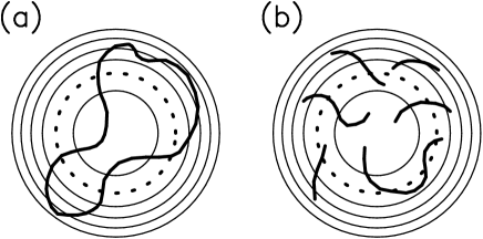
FIG. 4.: Single-lead scattering viewed on the surface of section. The circles represent channel tori selected by EBK quantization. If scattering is nonresonant a torus (dotted) is mapped into a closed curve [thick line in (a)]. In a resonant case (b), the mapping is discontinuous and the torus returns to the section as a set of fragments. This set may be infinite and even fractal.

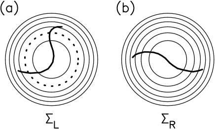
FIG. 5.: In multi-lead scattering the full surface of section is the union of the sections of all leads (two in this example). Shown is a torus in the left section [dotted, (a)] which is divided into a reflected part and a transmitted part [thick lines in (a) and (b), respectively].

FIG. 6.: A billiard connected to leads. Plot are a “standard” section $\Sigma_{0}$ and the Birkhoff section $\Sigma_{B}$. Thick lines represent the contour of the open billiard.

FIG. 7.: A scattering system discontinuous across a surface $\Sigma$. The sections $\Sigma_{L}$ and $\Sigma_{R}$ allow for isolating the problem of the discontinuity in the scattering from $\Sigma_{l}$ to $\Sigma_{r}$.

FIG. 8.: The “equivalent” one dimensional scattering problem for the discontinuity. A particle with energy $E$ propagates from the right channel $nR$ to the left channel $n^{\prime}L$ through the discontinuity $\Sigma$. The jump in the longitudinal momentum is $k_{n^{\prime}L}-k_{nR}$, where $\hbar^{2}k_{n^{\prime}L}^{2}/2m=E-\epsilon_{n^{\prime}L}$ and $\hbar^{2}k_{nR}^{2}/2m=E-\epsilon_{nR}$.

FIG. 9.: The semiseparable system consists of two waveguides: a semi-infinite one ($x<0$) and a finite one ($x>0$). Dirichlet conditions are assumed at $x=a$. Also shown are the auxiliary sections $\Sigma_{L}$ and $\Sigma_{0}$.

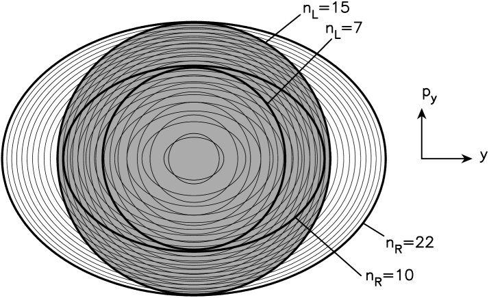
FIG. 10.: Quantized tori on each side of the semiseparable system. Circles correspond to channel modes and ellipses to cavity modes. The outermost circle corresponds to the last open channel.

FIG. 11.: Log₁₀-linear plot of the exact time delay $\tau(E)$, the section time delay $\tau_{0}(E)$, and the spectral determinant $D(E)$. The spikes at the bottom represent the energy levels of the bound system obtained by closing the cavity with a hard wall at $x=0$.

FIG. 12.: Elastic cross sections $|\mbox{\boldmath$S$}_{ii}|^{2}$ as a function of energy. Full lines correspond to the exact calculations. Dots represent the results of the “sudden approximation” (see text).

- [1] E. Bogomolny, Nonlinearity 5, 805 (1992).
- [2] C. Rouvinez and U. Smilansky, J. Phys. A 28, 77 (1995).
- [3] T. Prosen, J. Phys. A 28, 4133 (1995); Physica D 91, 244 (1996); and references therein.
- [4] C. H. Lewenkopf and H. A. Weidenmüller, Ann. Phys. 212, 53 (1991).
- [5] W. H. Miller, Adv. Chem. Phys. 25, 69 (1974).
- [6] A. M. Ozorio de Almeida and R. O. Vallejos, Chaos, Solitons & Fractals (to appear); also chao-dyn/9905010.
- [7] B. Georgeot and R. E. Prange, Phys. Rev. Lett. 74, 4110 (1995).
- [8] A. M. Ozorio de Almeida, Hamiltonian systems: Chaos and Quantization (Cambridge University Press, Cambridge, 1988).
- [9] H. A. Weidenmüller, Ann. Phys. 28, 60 (1964).