Spin-Gap States of a Periodic Mixed Spin Chain

Abstract

We examine a chain of periodic arrays of 4 quantum spins with magnitudes of 1/2, 1, 3/2 and 1. There are four kinds of nearest-neighbour exchange parameters among them. We choose two independent parameters for concreteness: one represents the ratio of typical exchange parameters, and the other represents a distortion. We determine the phase diagram of the ground state in the parameter space. The phase boundaries appear as gapless lines which separate gapful disordered phases. They are determined by the gapless equation which was previously derived by mapping a general periodic spin chain to the nonlinear $\sigma$ model.

1 Introduction

Since the discovery of cuprate superconductors, quantum spin systems have been studied to understand the magnetic properties of their undoped mother materials. In particular quantum spin systems with spin gap are interesting since the spin gap is possibly related to the superconducting gap in the doped case. Although the materials are two-dimensional, it is basically important to study magnetic properties of spin gap systems in any dimensions.

In one dimension, Haldane [1] predicted that the spin excitation spectrum of a uniform spin chain is gapless if the magnitude of a spin is a half-odd-integer, and is gapful if it is an integer. The prediction has been confirmed theoretically and experimentally in many standpoints. Since Haldane’s prediction is based on a mapping of a spin Hamiltonian to the nonlinear $\sigma$ model (NLSM), it is recognized that the NLSM is a useful tool to investigate spin systems.

The NLSM has been developed for periodic inhomogeneous spin chains. Affleck [2] derived and examined an NLSM for a spin chain with bond alternation. The application of the NLSM to spin chains with more than one spin species in the period of more than two lattice spacings are also considered [3, 4]. In particular we have succeeded to derive an NLSM, with accurately keeping the degrees of freedom of the spin variables, for a general mixed spin chain with arbitrary finite period [4].

We applied the NLSM method to systems with period 4 and spin species 2 (we defines the magnitudes as $s_{a}$ and $s_{b}$) [5, 6]. Imposing the condition that the ground state is singlet, only the possible order of spin magnitudes in a unit cell is of $s_{a}$-$s_{a}$-$s_{b}$-$s_{b}$. We obtained phase diagrams in the parameter space of the exchange couplings. In a few special cases, numerical calculations have been performed [7, 8, 9]. The phase diagrams obtained by the NLSM are qualitatively agree with the numerical results.

In this paper we examine another mixed spin chain with period 4 which includes three species of spins. The sequential order of magnitudes of spins in a unit cell is 1/2, 1, 3/2 and 1. There are four kinds of nearest-neighbour exchange couplings among them. If we consider a simplified case, the exchange parameters on the both sides of a 1/2 spin are the same value $J$, and those on the both sides of a 3/2 spin are of the same value $J^{\prime}$. We in fact consider the distortion of $J^{\prime}$ on the both sides of a 3/2 spin. We map the spin Hamiltonian describing the spin chain to an NLSM following Ref. [4]. From the value of the topological angle in the NLSM, we determine the phase diagram of this model in the space of the exchange parameters.

2 Mapping to the nonlinear $\sigma$ model

The Hamiltonian for the present spin chain is written as

$$H = \sum_{j}(J_{1}\,{\bf S}_{4j+1}\cdot{\bf S}_{4j+2}+J_{2}\,{\bf S}_{4j+2}\cdot{\bf S}_{4j+3}$$ (1)

$$+ J_{3}{\bf S}_{4j+3}\cdot{\bf S}_{4j+4}+J_{4}\,{\bf S}_{4j+4}\cdot{\bf S}_{4j+5}),$$

where the magnitudes of ${\bf S}_{4j+1}$, ${\bf S}_{4j+2}$, ${\bf S}_{4j+3}$ and ${\bf S}_{4j+4}$ are

$$(s_{1},s_{2},s_{3},s_{4})=\left(\frac{1}{2},1,\frac{3}{2},1\right).$$ (2)

A unit cell is illustrated in Fig. 1. To reduce the number of parameters, we restrict and reparametrize the antiferromagnetic exchange parameters as

$$J_{1}=J_{4}=J,\quad J_{2}=\frac{J^{\prime}}{1-\gamma},\quad J_{3}=\frac{J^{\prime}}{1+\gamma},$$ (3)

where $\gamma$ ($-1<\gamma<1$) is the distortion parameter describing the asymmetry between the couplings of the both sides of a spin with magnitude 3/2.

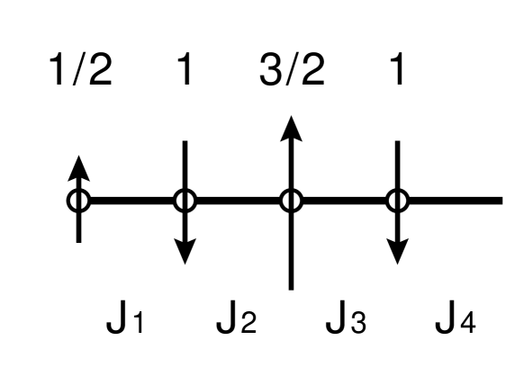
Figure 1: A unit cell of the 1/2-1-3/2-1 spin chain.

Following Ref. [4], we can map a general periodic mixed spin chain satisfying a restriction to the NLSM. The mapped NLSM action is given by

$$S_{\rm eff}= \int d\tau\int dx\biggl{\{}-i\frac{J^{(0)}}{J^{(1)}}{\bf m}\cdot\left(\frac{\partial{\bf m}}{\partial\tau}\times\frac{\partial{\bf m}}{\partial x}\right)$$ (4)

$$+\frac{1}{2aJ^{(1)}}\left(\frac{J^{(1)}}{J^{(2)}}-\frac{J^{(0)}}{J^{(1)}}\right)\left(\frac{\partial{\bf m}}{\partial\tau}\right)^{2}$$

$$+\frac{a}{2}J^{(0)}\left(\frac{\partial{\bf m}}{\partial x}\right)^{2}\biggl{\}},$$

where ${\bf m}$ is an O(3) unit-vector field and $a$ is the lattice constant. For a general spin chain with period $2b$, the constants in the action are given as follows:

$$\frac{1}{J^{(n)}} = \frac{1}{2b}\sum_{q=1}^{2b}\frac{({\tilde{s}}_{q})^{n}}{J_{q}s_{q}s_{q+1}}\quad(n=0,1,2)$$ (5)

with accumulated spins

$${\tilde{s}}_{q} = \sum_{k=1}^{q}(-1)^{k+1}s_{k}.\quad(q=1,2,\cdots,2b)$$ (6)

The action (4) is of the standard form of the NLSM:

$$S_{\rm st} = \int d\tau\int dx\biggl{\{}-i\frac{\theta}{4\pi}{\bf m}\cdot\left(\frac{\partial{\bf m}}{\partial\tau}\times\frac{\partial{\bf m}}{\partial x}\right)$$ (7)

$$+\frac{1}{2gv}\left(\frac{\partial{\bf m}}{\partial\tau}\right)^{2}+\frac{v}{2g}\left(\frac{\partial{\bf m}}{\partial x}\right)^{2}\biggl{\}},$$

where $\theta$ is the topological angle, $g$ is the coupling constant and $v$ is the spin wave velocity.

In the present model, the accumulated spins (6) are

$$({\tilde{s}}_{1},{\tilde{s}}_{2},{\tilde{s}}_{3},{\tilde{s}}_{4})=\left(\frac{1}{2},-\frac{1}{2},1,0\right)$$ (8)

and then the constants (5) are calculated as

$$\frac{1}{J^{(0)}}=\frac{1}{J}+\frac{1}{3J^{\prime}},$$

$$\frac{1}{J^{(1)}}=\frac{1}{4}\left(\frac{1}{J}+\frac{1}{3J^{\prime}}+\frac{\gamma}{J^{\prime}}\right),$$

$$\frac{1}{J^{(2)}}=\frac{1}{8}\left(\frac{1}{J}+\frac{5}{3J^{\prime}}+\frac{\gamma}{J^{\prime}}\right).$$ (9)

Figure 2: The topological angle $\theta$ as a function of $J^{\prime}/J$ for $\gamma$ = 0.0, 0.2, 0.4, 0.6, 0.8 and 1.0. The system is gapless on the lines of $\theta/\pi$ = 1 and 3 (dashed line).

Figure 3: The spin wave velocity $v$ as a function of $J^{\prime}/J$ for $\gamma$ = 0.0, 0.2, 0.4, 0.6, 0.8 and 1.0.

Figure 4: The coupling constant $g$ of the NLSM as a function of $J^{\prime}/J$ for $\gamma$ = 0.0, 0.2, 0.4, 0.6, 0.8 and 1.0.

Comparing Eq. (4) with Eq. (7), we have the topological angle

$$\theta=4\pi\frac{J^{(0)}}{J^{(1)}}=\pi+\frac{\pi\gamma}{\displaystyle\frac{J^{\prime}}{J}+\displaystyle\frac{1}{3}},$$ (10)

the spin wave velocity

$$v=\frac{4aJ^{\prime}}{\sqrt{\left(\displaystyle\frac{J^{\prime}}{J}+\displaystyle\frac{1}{3}\right)\left(\displaystyle\frac{J^{\prime}}{J}+3\right)-\gamma^{2}}}$$ (11)

and the coupling constant

$$g=\frac{4\left(\displaystyle\frac{J^{\prime}}{J}+\displaystyle\frac{1}{3}\right)}{\sqrt{\left(\displaystyle\frac{J^{\prime}}{J}+\displaystyle\frac{1}{3}\right)\left(\displaystyle\frac{J^{\prime}}{J}+3\right)-\gamma^{2}}}.$$ (12)

These quantities are shown in Figs. 2, 3 and 4, as functions of $J^{\prime}/J$ for several values of $\gamma$.

3 Phase diagram

It is well known that an NLSM has gapless excitations if the topological angle $\theta$ is an odd-integer multiple of $\pi$. In the general periodic spin model, this condition is turned into the gapless equation

$$\frac{2J^{(0)}}{J^{(1)}}=\frac{2l-1}{2}$$ (13)

with arbitrary integer $l$. In the present case of Eq. (10), it becomes of a simple form

$$\gamma=2l\left(\frac{J^{\prime}}{J}+\frac{1}{3}\right).\quad(l=-1,0,1)$$ (14)

The equation for each $l$ determines a phase boundary between gapful disordered phases. The restricted values of integer $l$ is due to the condition $-1<\gamma<1$. In the symmetric case of $\gamma=0$, the system is gapless irrespective of the ratio $J^{\prime}/J$, because it satisfies Eq. (14) with $l=0$.

The phase diagram of the ground state is obtained by identifying the gapless lines (14) as the phase boundaries. We show the phase diagram in Fig. 5. There exist four phases A₊, A_-, B₊ and B_- in the ($J^{\prime}/J$, $\gamma$) parameter space. The phase structure is symmetric for $\gamma\rightarrow-\gamma$ according to the symmetry of the Hamiltonian (1) with Eqs. (2) and (3).

In phase B₊, $\gamma$ is close to 1 and $J_{2}$ is selectively large. The ground state of B₊ may be explained by a VBS picture [10]. That is, if we decompose each spin into spins with magnitude 1/2, the ground state is approximately a direct product of dimers. Two dimers in a unit cell are formed between 1/2-spins at the both sides of a coupling with exchange parameter $J_{2}$. Phase A₊ is of an intermediate character and spreads over almost all area in the parameter space. The ground state of A₊ does not seem to be explained by the conventional VBS picture.

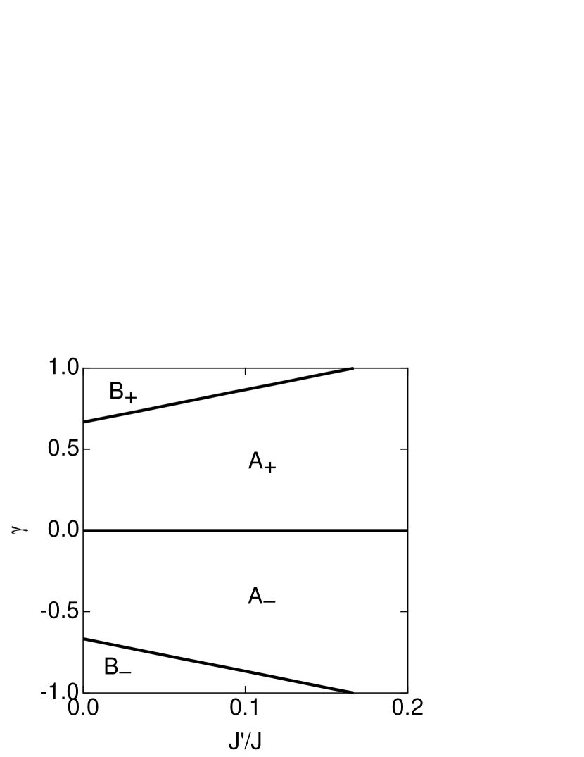
Figure 5: The phase diagram in the ($J^{\prime}/J$, $\gamma$) parameter space ($-1<\gamma<1$). The phase boundaries are gapless lines determined by Eq. (14).

4 Summary

We have examined the 1/2-1-3/2-1 spin chain with a distortion of the exchange parameters by using the nonlinear $\sigma$ model method. We obtained the phase diagram of the ground state in the parameter space. There exist four gapful phases. In the case of no distortion, the system is always gapless and is on a phase boundary. When the distortion is strong, there are two phases to be explained by a VBS picture. It is a future work to explain the other phases by the singlet-cluster-solid (SCS) picture developed in Ref. [6].

References

- [1] F.D.M. Haldane, Phys. Lett. 93 A (1983) 464; Phys. Rev. Lett. 50 (1983) 1153.
- [2] I. Affleck, Nucl. Phys. B 257 (1985) 397; 265 (1986) 409; I. Affleck, F.D.M. Haldane, Phys. Rev. B 36 (1987) 5291.
- [3] T. Fukui, N. Kawakami, Phys. Rev. B56 (1997) 8799.
- [4] K. Takano, Phys. Rev. Lett. 82 (1999) 5124.
- [5] K. Takano, to be published in Physica B (cond-mat/9909440).
- [6] K. Takano, to be published in Phys. Rev. B (cond-mat/9911098).
- [7] W. Chen, K. Hida, J. Phys. Soc. Jpn. 67 (1998) 2910.
- [8] T. Hikihara, T. Tonegawa, M. Kaburagi, T. Nishino, S. Miyashita, H.-J. Mikeska, preprint.
- [9] T. Tonegawa, T. Hikihara, M. Kaburagi, T. Nishino, S. Miyashita, H.-J. Mikeska, J. Phys. Soc. Jpn. 67 (1998) 1000.
- [10] I. Affleck, T. Kennedy, E. H. Lieb, H. Tasaki, Phys. Rev. Lett. 59 (1987) 799.