Spontaneous deformation of the Fermi surface due to strong correlation in the two-dimensional $t$-$J$ model

Abstract

Fermi surface of the two-dimensional $t$-$J$ model is studied using the variational Monte Carlo method. We study the Gutzwiller projected $d$-wave superconducting state with an additional variational parameter $t^{\prime}_{\rm v}$ corresponding to the next-nearest neighbor hopping term. It is found that the finite $t^{\prime}_{\rm v}<0$ gives the lowest variational energy in the wide range of hole-doping rates. The obtained momentum distribution function shows that the Fermi surface deforms spontaneously. It is also shown that the van Hove singularity is always located very close to the Fermi energy. Using the Gutzwiller approximation, we show that this spontaneous deformation is due to the Gutzwiller projection operator or the strong correlation.

71.10.Fd, 71.10.Pm, 79.60.-i

The effect of strong correlation is one of the most important issues for understanding the high-$T_{c}$ superconductivity (SC). Among various anomalous electronic properties, the experiments of angle resolved photoemission spectroscopy (ARPES) have revealed that a flat band around ($\pi$, 0) and (0, $\pi$) is pinned just below the Fermi energy.[2, 3, 4] This phenomenon is unexpected in the band calculations and it is considered to be closely related to the opening of the pseudogap on the Fermi surface (FS) [5, 6, 7], which is also an extraordinary feature in high-$T_{c}$ cuprates. This anomalous nature of the FS will be the direct evidence for the non-Fermi liquid behavior. It is thus an interesting issue to study the FS in the presence of strong correlation.

The effect of the flat band and the geometry of the FS can be taken into account by using the $t$-$t^{\prime}$-$J$ model or the $t$-$t^{\prime}$-$U$ Hubbard model in which the next-nearest neighbor hopping term $t^{\prime}$ is introduced as a fitting parameter.[8] If one chooses $t^{\prime}<0$, the FS centered at ($\pi$, $\pi$) observed experimentally[4, 9] can be reproduced in the tight-binding model. However high temperature expansion studies on the momentum distribution function for the $t$-$J$ model[10] have shown that the FS is similar to that with $t^{\prime}<0$ even though the $t^{\prime}$-term is absent in the Hamiltonian. On the other hand, the conventional mean-field theories, such as slave-boson theory, simply give the FS with $t^{\prime}=0$. Therefore the strong correlation which is not included in the mean-field theories will be the origin of the change of the FS geometry.

Here we study this problem from a different point of view. Since the calculation in Ref.[10] is carried out in the high temperature region, it is not clear whether or not the FS deforms down to zero temperature. To study the FS of the ground state is generally very difficult. The exact diagonalization study of small clusters does not give enough resolution in the $k$ space. The quantum Monte Carlo simulations have been often useless for the two-dimensional $t$-$J$ model because of the minus sign problem. Therefore we use the variational Monte Carlo (VMC) method in this paper, which is free from the limitation of the system size as well as from the sign problem. The VMC method treats exactly the constraints of no doubly occupied sites and gives accurate estimates of the expectation values such as the variational energies and the momentum distribution functions.

Although it is a variational theory, the VMC method is powerful to see whether some kind of symmetry breaking takes place or not. In this paper we examine the Gutzwiller-projected $d$-wave superconducting state which contains an additional variational parameter $t^{\prime}_{\rm v}$ corresponding to the next-nearest neighbor hopping term. We can safely discuss the relative energy difference between the variational states with and without $t^{\prime}_{\rm v}$, although the absolute values of the variational energies can still be lowered. We find that the wave function with $t^{\prime}_{\rm v}\sim-0.1$ has the lowest variational energy even though the Hamiltonian does not contain $t^{\prime}$-term. This means that the FS deforms spontaneously. The momentum distribution function $n(\mbox{\boldmath$k$})$ calculated in the optimized wave function is consistent with that in the high temperature expansion. Our method gives an independent and complementary support of the result that the deformation of the FS is a distinctive feature of strongly correlated electron systems.

In addition to this, we can identify the physical origin of the FS deformation in our variational approach. We show the relation between the energy gain and the van Hove singularity. It has been argued that a remarkable enhancement of SC correlation is achieved if the van Hove singularity is close to the Fermi energy.[11, 12] Our results show some similarity to this picture. Furthermore, by comparing the obtained results with the Gutzwiller approximation, we can see that the finite $t^{\prime}_{\rm v}$ is caused solely by the Gutzwiller projection.

We use the two-dimensional $t$-$J$ model on a square lattice,

$$H=-t\sum_{\langle ij\rangle\sigma}P_{\rm G}(c_{i\sigma}^{\dagger}c_{j\sigma}+h.c.)P_{\rm G}+J\sum_{\langle ij\rangle}\mbox{\boldmath$S$}_{i}\cdot\mbox{\boldmath$S$}_{j},$$ (1)

where $\langle ij\rangle$ represents the sum over the nearest-neighbor sites. $c_{i\sigma}^{\dagger}$ ($c_{i\sigma}$) is a creation (annihilation) operator of $\sigma$ ($\uparrow$ or $\downarrow$) electron at $i$-site and $\mbox{\boldmath$S$}_{i}=c_{i\alpha}^{\dagger}(\frac{1}{2}\mbox{\boldmath$\sigma$})_{\alpha\beta}c_{i\beta}$. The Gutzwiller’s projection operator $P_{\rm G}$ is defined as $P_{\rm G}=\Pi_{i}(1-\hat{n}_{i\uparrow}\hat{n}_{i\downarrow})$, which prohibits the doubly occupied sites. We set $J/t=0.3$.

We use a Gutzwiller-projected mean-field type wave function $P_{\rm G}P_{N_{\rm e}}|\phi_{0}\rangle$ as a trial state with fixing the number of electrons $N_{\rm e}$ through $P_{N_{\rm e}}$. The state is written as

$$P_{\rm G}P_{N_{\rm e}}|\phi_{0}\rangle = P_{\rm G}P_{N_{\rm e}}\prod_{k}(u_{k}+v_{k}c_{k\uparrow}^{\dagger}c_{-k\downarrow}^{\dagger})|0\rangle$$ (2)

$$= P_{\rm G}P_{N_{\rm e}}\prod_{k}u_{k}\exp\left[\sum_{k}\frac{v_{k}}{u_{k}}c_{k\uparrow}^{\dagger}c_{-k\downarrow}^{\dagger}\right]|0\rangle$$ (3)

$$= P_{\rm G}P_{N_{\rm e}}\prod_{k}u_{k}\exp\left[\sum_{ij}a_{ij}c_{i\uparrow}^{\dagger}c_{j\downarrow}^{\dagger}\right]|0\rangle$$ (4)

$$= P_{\rm G}\prod_{k}u_{k}\frac{1}{(N_{\rm e}/2)!}\left(\sum_{ij}a_{ij}c_{i\uparrow}^{\dagger}c_{i\downarrow}^{\dagger}\right)^{N_{\rm e}/2}|0\rangle,$$ (5)

where $v_{k}/u_{k}=\Delta_{k}/(\epsilon_{k}-\mu+\sqrt{(\epsilon_{k}-\mu)^{2}+\Delta_{k}^{2}})$ and $a_{ij}$ is a Fourier transform of $v_{k}/u_{k}$.

Usually $\epsilon_{k}$ is chosen to be $\epsilon_{k}=-2(\cos k_{x}+\cos k_{y})$, which is in accordance with the Hamiltonian (1). However in this paper, we introduce an additional variational parameter $t^{\prime}_{\rm v}$ which changes the FS of the variational state. We assume $\epsilon_{k}$ and $\Delta_{k}$ as

$$\epsilon_{k} = -2(\cos k_{x}+\cos k_{y})-4t^{\prime}_{\rm v}\cos k_{x}\cos k_{y},$$ (6)

$$\Delta_{k} = 2\Delta_{d}(\cos k_{x}-\cos k_{y}).$$ (7)

The present wave function contains three variational parameters $t^{\prime}_{\rm v}$, $\mu$ and $\Delta_{d}$.

At first, using the above wave function we calculate the variational energy $E_{\rm var}$ of the Hamiltonian (1)

$$E_{\rm var}=\frac{\langle\phi_{0}|P_{N_{\rm e}}P_{\rm G}HP_{\rm G}P_{N_{\rm e}}|\phi_{0}\rangle}{\langle\phi_{0}|P_{N_{\rm e}}P_{\rm G}P_{\rm G}P_{N_{\rm e}}|\phi_{0}\rangle},$$ (8)

by means of the VMC method. The distribution of the wave vectors $k$ is determined in the periodic boundary conditions in the $x$ direction and in the antiperiodic ones in the $y$ direction so as to avoid the gap node of $d$-wave superconductivity. Although the results in the 10$\times$10 square lattice are mainly shown in the following, we also calculate larger sizes up to $20\times 20$ to investigate the size dependence.

FIG. 1.: $\Delta_{d}$ dependence of $E_{\rm var}/t$ for $t^{\prime}_{\rm v}=0$ (open squares), $-0.05$ (filled squares), $-0.1$ (open circles) and $-0.15$ (filled circles). Each point has been minimized with respect to $\mu$. System size is 10$\times$10 and the number of Monte Carlo samples is $2.5\times 10^{5}$.

Figure 1 shows the $\Delta_{d}$ dependence of $E_{\rm var}$ for various values of $t^{\prime}_{\rm v}$ at the doping rate $\delta=0.12$. Apparently $t^{\prime}_{\rm v}\sim-0.1$ gives the lowest variational energy. Since the Hamiltonian does not contain next-nearest neighbor hopping terms, the present result means that the shape of the FS of the ground state is different from that of the non-interacting Hamiltonian. We have also checked that, if the Hamiltonian has the next-nearest neighbor hopping term $t^{\prime}$, the optimized variational state has $t^{\prime}_{\rm v}$, whose amplitude is larger than $t^{\prime}$.

The most significant effect of this result appears in the shape of momentum distribution functions. Figure 2 shows a contour map of the gradient of the momentum distribution function $|\nabla_{k}n(\mbox{\boldmath$k$})|$ for $t^{\prime}_{\rm v}=-0.1$ calculated on the 20$\times$20 square lattice. Although we have used the optimized variational parameters $\Delta_{d}$ and $\mu$ on the 10$\times$10 lattice, it is justified because their size dependeces are negligible. Brighter areas in Fig. 2 correspond to the momentum $k$ with larger values of $|\nabla_{k}n(\mbox{\boldmath$k$})|$. Although we cannot specify exactly the location of the FS due to the $d$-wave SC gap, we expect that the FS lies close to the area where $|\nabla_{k}n(\mbox{\boldmath$k$})|$ is large.

Our result of momentum distribution function is similar to that obtained in high temperature expansion by Putikka et al.[10] Since we take an opposite approach to high temperature studies, i.e., in the zero temperature, it is confirmed that the FS shown in Fig. 2 is an intrinsic feature of the $t$-$J$ model. Note here that the smearing of the FS around ($\pi$, 0) in our calculation is due to the $d$-wave SC gap. This suggests that the similar smearing observed in Ref.[10] may be due to the pseudogap with $d$-wave symmetry, in addition to the smearing due to finite temperature.

For the wide range of doping $\delta=0.04\sim 0.20$, we find that $E_{\rm var}$ is minimized around $t^{\prime}_{\rm v}\sim-0.1$ and the chemical potential $\mu\sim-0.5\pm 0.05$. Because of the insensitiveness of $\mu$ as a function of doping, the area of the momentum space enclosed by the FS is also insensitive to the doping rate. This result supports the violation of the Luttinger theorem suggested by Putikka et al.[10] Actually $n(\mbox{\boldmath$k$})$ at the doping $\delta=0.2$ in Ref.[10] is very close to our results in Fig. 2 at $\delta=0.12$.

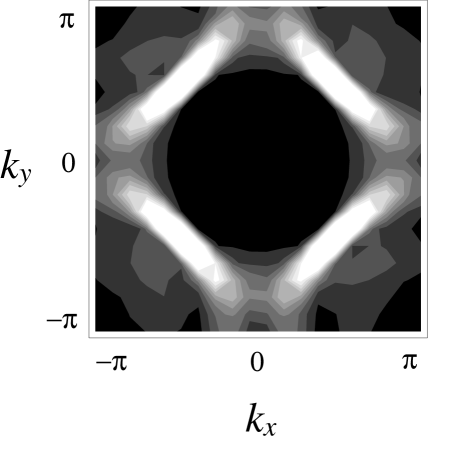
FIG. 2.: Full Brillouin zone plot of $|\nabla_{k}n(k)|$ for the doping rate $\delta=0.12$ and $J/t=0.3$. The areas with large values of $|\nabla_{k}n(k)|$ are highlighted. Note that the FS is deformed even though the Hamiltonian does not contain the next-nearest neighbor hopping terms. The smearing near ($\pi$, 0) and (0, $\pi$) is due to the presence of the $d$-wave SC order parameters.

Figure 3 shows the energy difference between the value at $t^{\prime}_{\rm v}=0$ and at $t^{\prime}_{\rm v}=-0.1$, i.e. the energy gain due to the finite $t^{\prime}_{\rm v}$, for several system sizes. Although the Monte Carlo results scatter a little, there is apparently a tendency that the energy gain due to the finite $t^{\prime}_{\rm v}$ becomes maximum around $\delta=0.12$. As we increase the system size, the energy gain slightly decreases, but it will remain finite in the thermodynamic limit.

FIG. 3.: Doping dependence of the energy gain at $t^{\prime}_{\rm v}=-0.1$ compared with $t^{\prime}_{\rm v}=0$. The system sizes are $10\times 10$ (open squares), $12\times 12$ (filled squares) and $14\times 14$ (open circles). The number of samples is more than 10⁵.

Let us discuss here the relation between the energy gain and the van Hove singularity. For the optimized value $t^{\prime}_{\rm v}\sim-0.1$, $\epsilon_{k}$ at $\mbox{\boldmath$k$}=(\pi,0)$ becomes $-0.4$. On the other hand, the optimized chemical potential $\mu$ is around $-0.5$. This means that the suddle point or the position of the flat band near $\mbox{\boldmath$k$}=(\pi,0)$ is very close to the chemical potential. Since the $d$-wave SC gap has a maximum at $(\pi,0)$, the enhancement of the density of states near the Fermi energy due to the van Hove singularity causes the energy gain. Actually, if we assume $\Delta_{d}=0$, the lowest energy is achieved at $t_{\rm v}^{\prime}=0$. This indicates that the FS deforms itself so as to fix the van Hove singularity to the chemical potential in the presence of the $d$-wave SC gap. This looks consistent with the mechanism of SC due to the van Hove singularity.[11, 12]

If we use a Hamiltonian $\tilde{H}_{t{\mbox{-}}J}$ without projection operator and the mean-field wave function $|\phi_{0}\rangle$, it is apparent that the variational energy $\langle\phi_{0}|\tilde{H}_{t{\mbox{-}}J}|\phi_{0}\rangle/\langle\phi_{0}|\phi_{0}\rangle$ is minimized at $t^{\prime}_{\rm v}=0$. Therefore the energy gain due to the non-zero value of $t^{\prime}_{\rm v}$ is solely from the Gutzwiller’s projection operator. In order to clarify the effect of the projection, we examine the Gutzwiller approximation[13], in which the effect of constraints are taken into account by statistical weighting factors. For the $t$-$J$ model, we have

$$\frac{\langle\phi_{0}|P_{\rm G}c_{i\sigma}^{\dagger}c_{j\sigma}P_{\rm G}|\phi_{0}\rangle}{\langle\phi_{0}|P_{\rm G}P_{\rm G}|\phi_{0}\rangle}=g_{t}\langle\phi_{0}|c_{i\sigma}^{\dagger}c_{j\sigma}|\phi_{0}\rangle=g_{t}\langle c_{i\sigma}^{\dagger}c_{j\sigma}\rangle_{0}$$ (9)

and

$$\frac{\langle\phi_{0}|P_{\rm G}\mbox{\boldmath$S$}_{i}\cdot\mbox{\boldmath$S$}_{j}P_{\rm G}|\phi_{0}\rangle}{\langle\phi_{0}|P_{\rm G}P_{\rm G}|\phi_{0}\rangle}=g_{s}\langle\phi_{0}|\mbox{\boldmath$S$}_{i}\cdot\mbox{\boldmath$S$}_{j}|\phi_{0}\rangle=g_{s}\langle\mbox{\boldmath$S$}_{i}\cdot\mbox{\boldmath$S$}_{j}\rangle_{0},$$ (10)

where $g_{t}$ and $g_{s}$ are the renormalization factors due to the projection. In the simplest Gutzwiller approximation, $g_{t}$ and $g_{s}$ are constant, i.e., $g_{t}=2\delta/(1+\delta)$ and $g_{s}=4/(1+\delta)^{2}$. [13] In this case, the Gutzwiller projection does not alter the mean-field results. However it was recently shown that the dependence of the renormalization factors on the expectation values, such as $\chi=\langle c_{i\sigma}^{\dagger}c_{j\sigma}\rangle_{0}$ and $\Delta=\langle c_{i\uparrow}^{\dagger}c_{j\downarrow}^{\dagger}\rangle_{0}$, plays a crucial role in evaluating the variational energies. [14, 15, 16, 17] If we use this Gutzwiller approximation, we can show that

$$\delta E_{\rm var}\propto\frac{\partial\langle H\rangle}{\partial\chi^{\prime}}\delta t_{\rm v}^{\prime}+8Nt_{\rm v}^{\prime}\delta t_{\rm v}^{\prime}$$ (11)

where $\chi^{\prime}=\langle c_{i\sigma}^{\dagger}c_{j\sigma}\rangle_{0}$ with $(ij)$ being the next-nearest neighbor sites and

$$\frac{\partial\langle H\rangle}{\partial\chi^{\prime}}\equiv-t\frac{\partial g_{t}}{\partial\chi^{\prime}}\sum_{\langle ij\rangle\sigma}(\langle c_{i\sigma}^{\dagger}c_{j\sigma}\rangle_{0}+c.c.)+J\frac{\partial g_{s}}{\partial\chi^{\prime}}\sum_{\langle ij\rangle}\langle\mbox{\boldmath$S$}_{i}\cdot\mbox{\boldmath$S$}_{j}\rangle_{0}.$$ (12)

The first term on the r.h.s. of eq. (11) is linear with respect to $t_{\rm v}^{\prime}$ so that $E_{\rm var}$ is minimized at a finite value of $t_{\rm v}^{\prime}$ which satisfies

$$t_{\rm v}^{\prime}=-\frac{1}{8N}\frac{\partial\langle H\rangle}{\partial\chi^{\prime}}.$$ (13)

Apparently the renormalization factors $g_{t}$ and $g_{s}$ due to the projection operator and their nonlinear dependence on $\chi^{\prime}$ are the origin of the spontaneous deformation of the FS. These phenomena cannot be found in the mean-field theories. The explicit calculations will be published elsewhere.

In summary, we investigated the shape of the FS in the two-dimensional $t$-$J$ model by means of the VMC calculation introducing an additional variational parameter $t^{\prime}_{\rm v}$. We found that the variational energy is minimized around $t^{\prime}_{\rm v}\sim-0.1$ for various doping rates. The system size dependence indicate this effect is realized even in the thermodynamic limit. The magnitude of the energy gain is large enough compared with other VMC studies. For example, the energy difference between the pure $d$-wave SC phase and the coexistent phase of AF and $d$-wave SC is comparable to the present energy gain at the doping rate $\delta\sim 0.08$.[16, 18] Then we have clarified the origin of the energy gain by examining the van Hove singularity and the effect of the projection using the Gutzwiller approximation. Combining our results at zero temperature and those in high temperature expansion, we consider that the FS deformation is the most significant phenomenon in the presence of strong correlation.

Since the nesting property of the FS becomes worse in the present wave function than in the original $t$-$J$ model, the coexistence of AF and $d$-wave SC near half-filling[16, 18] will be suppressed. Alternatively we expect some incommensurate AF correlations which were unexpected in the $t$-$J$ model. This is presumably related to the stripe state observed experimentally.

REFERENCES

- [1]
- [2] D. S. Dessau, Z.-X. Shen, D. M. King, D. S. Marshall, L. W. Lombardo, P. H. Dickinson, A. G. Loeser, J. DiCarlo, C.-H. Park, A. Kapitulnik and W. E. Spicer, Phys. Rev. Lett. 71, 2781 (1993).
- [3] D. S. Marshall, D. S. Dessau, A. G. Loeser, C.-H. Park, A. Y. Matsuura, J. N. Eckstein, I. Bozovic, P. Fournier, A. Kapitulnik, W. E. Spicer and Z.-X. Shen, Phys. Rev. Lett. 76, 4841 (1996).
- [4] A. Ino, C. Kim, T. Mizokawa, Z.-X. Shen, A. Fujimori, M. Takaba, K. Tamasaku, H. Eisaki and S. Uchida, J. Phys. Soc. Jpn. 68, 1496 (1999).
- [5] H. Yasuoka, T. Imai and T. Shimizu, in Strong Correlation and Superconductivity, edited by H. Fukuyama, S. Maekawa and A. P. Malozemoff (Springer 1989) p254.
- [6] J. Rossat-Mignot, L. P. Regnault, C. Vettier, P. Burlet, J. Y. Henry and G. Lapertot, Physica B 169, 58 (1991); J. Rossat-Mignot, L. P. Regnaut, P. Bourges, P. Burlet, L. Vettier and J. Y. Henry, ibid. 192, 109 (1993).
- [7] M. R. Norman, H. Ding, M. Randeria, J. C. Campuzano, T. Yokoya, T. Takahashi, T. Mochiku, K. Kadowaki, P. Guptasarma and D. G. Hinks, Nature 392, 157 (1998).
- [8] T. Tanamoto, H. Kohno and H. Fukuyama, J. Phys. Soc. Jpn. 62, 717 (1993).
- [9] P. Aebi, J. Osterwalder, P. Schwaller, L. Schlapbach, M. Shimoda, T. Mochiku and K. Kadowaki, Phys. Rev. Lett. 72, 2757 (1994).
- [10] W. O. Putikka, M. U. Luchini and R. R. P. Singh, Phys. Rev. Lett. 81, 2966 (1998).
- [11] L. F. Feiner, J. H. Jefferson and R. Raimondi, Phys. Rev. Lett. 76, 4939 (1996).
- [12] K. Yamaji, T. Yanagisawa, T. Nakanishi and S. Koike, Physica C 304, 225 (1998).
- [13] F. C. Zhang, C. Gros, T. M. Rice and H. Shiba, Supercond. Sci. Technol. 1, 36 (1988).
- [14] T. C. Hsu, Phys. Rev. B 41, 11379 (1990).
- [15] M. Sigrist, T. M. Rice and F. C. Zhang, Phys. Rev. B 49, 12058 (1994).
- [16] A. Himeda and M. Ogata, Phys. Rev. B 60, R9935 (1999).
- [17] M. Ogata and A. Himeda, in preparation.
- [18] T. Giamarchi and Lhuillier, Phys. Rev. B 43, 12943 (1991).