Effects of spin-elastic interactions in frustrated Heisenberg antiferromagnets
Abstract
The Heisenberg antiferromagnet on a compressible triangular lattice in the spin-wave approximation is considered. It is shown that the interaction between quantum fluctuations and elastic degrees of freedom stabilize the low symmetric L-phase with a collinear Néel magnetic ordering. Multi-stability in the dependence of the on-site magnetization is on an uniaxial pressure is found.
There is a long standing interest in properties of frustrated quantum antiferromagnets because they display a large variety of behavior: e.g. conventional spin ordering, spin liquid ground states, or chirality transitions [1]. The antiferromagnetic Heisenberg model on a triangular lattice is the simplest two-dimensional frustrated system. Quasi-two-dimensional triangular lattice antiferromagnets are not rare objects. It was recently shown [2, 3] that the materials belonging to the Yavapaiite family may be considered as realizations of a quasi-two-dimensional triangular lattice quantum (e.g. M=Ti with S=1/2) and quasiclassical (e.g. M=Fe with S=5/2) antiferromagnets. The rhombohedral -phase and monoclinic -phase of solid oxygen consist of weakly interacting planes (triangular in the case of and rectangular in the case of [5]) whose magnetic properties are described by the easy-plane Heisenberg antiferromagnetic model with spin [4].
Unconventional properties of the family can be described by a Hubbard model on a triangular lattice with an anisotropic interactions [6]. An antiferromagnetic Heisenberg model was also used in [7] to describe the properties of a triangular monolayer of Pb and Sn adatoms on the (111) surface of Ge form.
From the theoretical point of view the antiferromagnetic Heisenberg model on a triangular lattice has attracted particular attention since Anderson’s proposal of a resonance-valence-bond state for this model [8]. From that time much work has been done to understand the nature of its ground state. There is now an almost consensus based on variety of methods [9, 10, 11, 12] that the ground state has a conventional three-sublattice order but the situation is close to marginal and quantum fluctuations are important [13]. Quite recently the effect of quantum spin fluctuations on the ground-state properties of spatially anisotropic Heisenberg antiferromagnet in the linear spin-wave approximation was explored [14, 15, 16]. The staggered magnetization and the magnon dispersion were calculated as functions of the ratio of the antiferromagnetic exchange between the second and first neighbors,. As a physical tool which allows to tune the ratio Merino et al [16] invoke an uniaxial stress within a layer whereby the relative distances between atoms are changed.
In this paper we investigate the ground-state properties of the compressible frustrated antiferromagnets, i.e. those systems where the coupling between magnetic and elastic degrees of freedom is taken into account,under the action of uniaxial pressure. We treat the system self-consistently considering the spin subsystem in the linear spin-wave approximation and using the continuum approach for the elastic degrees of freedom. We show that as a result of this method the behavior of the on-site magnetization as a function of the pressure differs significantly from the behavior which was obtained in the framework of the spatially anisotropic Heisenberg model [15, 16]. In particular, the on-site-magnetization does not vanish in the whole interval of stability of the collinear phase.
We consider the two-dimensional triangular lattice. The Hamiltonian of the spin subsystem, interacting with the displacements of the magnetic atoms, is
| (1) |
Here is the spin operator of the atom located in the -th site of the triangular lattice: where are the basic vectors of the triangular lattice, is the exchange integral ( is the exchange constant), are the atom displacements from their equilibrium (without magnetic interaction), and is the vector which connects a site with nearest neighbors, . We consider a small spatially smooth deformation. Therefore it was convenient to introduce the components of the strain tensor : (
The elastic energy of the two-dimensional triangular lattice in the continuum approximation coincides with the elastic energy of the isotropic plane: where and are the elastic modulus of the system and are the component of the uniaxial pressure.
Let us use the transformation (see e.g. [17]) to the local frame of reference in which quantization axis for the spins at each site coincide with its classical direction which is determined by the vector . By using the Holstein-Primakoff spin-representation with , being the creation (destruction) Bose-operator of the spin-excitation on the -th site and applying the Bogolyubov transformation for these operators ( is the wave vector belonging to the first Brillouin zone and is the number of atoms in the crystal), the Hamiltonian (1) in the spin-wave approximation can be represented in the form where
| (2) |
is the ground state energy per atom in the spin-wave approximation. The coefficients of the Bogolyubov transformation are given by where
| (3) | |||
| (4) |
with , and
| (5) |
is the magnon energy. is the energy of the spin subsystem per atom in the classical approximation.
The on-site magnetization can be also obtained by using the Bogolyubov transformation. As a result we get
| (6) |
Our goal now is to minimize the total ground state energy of the system
| (7) |
with respect to the variational parameters which are the components of the deformation tensor and the vector . Here the magneto-elastic constant characterizes the stiffness of the lattice in terms of the intensity of the spin-lattice interaction, is the dimensionless uniaxial pressure. In Eq. (7) we omitted the terms of spin-lattice interaction which correspond to the dilatation (contraction) of the lattice () without changing its symmetry. These terms don’t change the qualitative behavior of the system. The equations for and have the form
| (8) |
Let us consider first the case zero pressure: . In the classical approximation when the energy of the system can be represented in the form
| (9) |
i) H-phase: The spin structure corresponding to each is a three-sublattice antiferromaget.Three different represent three possible antiferromagnetic domains. The lattice structure is an undistorted triangular lattice with the group symmetry .
ii) L-phase: The spin structure corresponding to each is a two-sublattice antiferromagnet. The lattice structure for is determined by the deformation tensors while for two other the deformation tensors can be obtained by rotations by . The lattice is characterized by the group symmetry .
iii) S-phase: where . Two more vectors and deformation tensors and can be obtained from the above equation by rotations by . The spin structure is a spiral antiferromagnet.
We consider the stability of obtained solutions for the case when
| (10) |
In the subspace (10) the stability condition reads
| (11) |
One can obtain from Eqs (9) and (11) that
-
the -phase is stable when
-
both - and -phases are stable when For the H- and L-phases have the same energy while for the L-phase becomes energetically more favorable.
-
the -phase is stable when .
The spiral S-phase does not correspond to a minimum of the ground state energy. In the subspace (10) the spiral phase for corresponds to the saddle point which separates two stable phases and .
The wave vectors and determine also the magnetic structure of the H- and L-phases in the spin-wave approximation. This is not true, however, for the spiral phase where quantum fluctuations change the value of the spiral wave-vector .
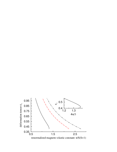
for the collinear L-phase (full curve S=1/2,dashed curve S=1,
dotted-dashed curve S=3/2) as a function of the renormalized
magneto-elastic constant . Multistability for
the case S=1/2 is shown in the inset.
Evaluating numerically the integrals in the r.h.s. of Eq. (2) for one can obtain that the ground state energy of the symmetric triangular phase in the spin-wave approximation is . We have also found that the H-phase is stable for where
| (12) |
Considering the low-symmetry L-phase which corresponds to the wave vector we obtain from Eqs (3), (5) that its energy in the spin-wave approximation is determined by the expression
| (13) | |||
| (14) |
where is the elliptic integral of the second kind [19] with the parameter . One can obtain from Eq. (5) that in the limit the magnon dispersion in the L-phase has the form . This means that the magnons in the low-symmetry L-phase can exist only for and only in this interval we may look for extrema of the function . It is seen from Eqs (1) that the quantity corresponds to the antiferromagnetic exchange between first (second) neighbors in the spin-wave theory of Heisenberg antiferromagnet on an anisotropic triangular lattice [15, 16]. Therefore the interval corresponds to the interval in the spin-wave theory of Heisenberg antiferromagnet on an anisotropic triangular lattice.
In Fig. 1 we plot the deformation tensor which provides an extremum of , as a function of the coupling parameter for three spin values . It is seen that the equation has solution only for . The critical value which determines the interval of the existence of the L-phase depends on the spin . It increases when the spin increases, e.g.
| (15) |
but even for it is still less () than the critical value for this parameter obtained in the classical approximation (). The reason for this is the strong contribution to the effective elastic energy of the system from quantum fluctuations (the second term in the r.h.s. of Eq. (13)).The quantum fluctuations change both the stiffness of the lattice (the second derivative of the free energy (13) with respect to the deformation ) and the constant of the spin-elastic interaction ( the first derivative of the free energy). A single-valued monotonic dependence is obtained for . For the dependence becomes multi-valued, i.e. there is an interval of where two values and ( ) of the deformation tensor correspond to each value of the coupling constant . Only the solution which corresponds to the deformation corresponds to the minimum of the effective elastic energy (13).
To find the stability region of the collinear L-phase we numerically evaluated integrals in the l.h.s. of the inequality (11) and found that it holds in the interval . Comparing the stability limits for H- and L-phases give in Eqs (12) and (15) we find the following interesting results. For we have always like in the classical approach where the stability regions for H- and L-phases overlap. However, for this is not the case since there is an interval where neither the L- nor the H-phase exist.
The nature of the phase in the interval or in other words for , cannot be clarified in the framework of the spin-wave approach. The reason why this approach fails is the following. As it was mentioned above the vectors obtained in the classical approach are not solutions of the extrema conditions (8) in the spin-wave approximation. On the other hand, as it is seen from Eqs (5) and (3) the magnon frequency is real in the interval only for obtained in the classical approach. For other values is not positive definite. Thus to check the stability of the corresponding phase is stable one should calculate the magnon dispersion beyond the spin-wave approach.

magnetization in the L-phase (). The
inset represents the magnetization as a function of the
ratio of the effective exchange
integrals between the second and first neighbors in the
presence of the uniaxial pressure.
Let us consider how the L-phase evolves in the presence of an uniaxial pressure . From Eqs (7) and (8) we get
| (16) | |||
| (17) |
In Fig. 2 we show results for the on-site magnetization in the L-phase for as a function of the uniaxial pressure . Fig. 2 and in particular its inset shows that our results are qualitatively different from those of a recent spatially anisotropic triangular lattice study [15, 16]. In contrast to the -model [15, 16] where the ratio was a free parameter in our model the corresponding parameter in a compressible triangular lattice is determined self-consistently from the extrema conditions (8). It is seen that in the interval of the existence of the L-phase we have ) and the on-site magnetization is finite. It is interesting that there exists an interval where two values of the magnetization correspond to each value of the pressure . One can show, however, that only the state with a larger value of is stable.
We conclude that the Heisenberg antiferromagnet on an compressible triangular lattice differs qualitatively from the Heisenberg antiferromagnet on an anisotropic triangular lattice. Self-consistent treatment of the elastic degrees of freedom shows that the spiral magnetic phase is unstable in the classical approximation. This approach shows also that in the spin-wave approximation the interaction between quantum fluctuations and elastic degrees of freedom stabilizes the collinear L-phase.
Acknowledgements
Yu. Gaididei is grateful for the hospitality of the University of Bayreuth
where this work was performed. Partial support from the DRL grant Nr.: UKR-002-99 is also acknowledged.
REFERENCES
- [1] Magnetic Systems with Competing Interactions, edited by H.T. Diep (World Scientific, Singapore, 1994).
- [2] S.T. Bramwell, S.G. Carling, C.J. Harding, K.D.M. Harris, B.M. Kariuki, L. Nixon, and I.P. Parkin, J.Phys.: Condens. Matter. 8, L123 (1996).
- [3] H. Serrano-González, S.T. Bramwell, K.D.M. Harris, B.M. Kariuki, L. Nixon, I.P. Parkin, and C. Ritter, Phys. Rev. B 59, 14451 (1999).
- [4] Yu.B. Gaididei, V.M. Loktev, A.F. Prikhotko, and L.I. Shansky, Sov. J. Low Temp. Phys. 1,653 (1975) (Fiz. Nizk. Temp. 1, 1365 (1975)).
- [5] I. N. Krupskii, A. I. Prokhvatilov, Yu. A. Freiman, and A. I. Erenburg, Sov. J. Low Temp. Phys. ,130 (1979) (Fiz. Nizk. Temp. 5, 271 (1979)).
- [6] R.H. McKenzie, Comment. Condens. Matter Phys. 18, 309 (1998).
- [7] J.P. Rodriguez and E. Artacho, Phys.Rev. B 59, R705 (1999).
- [8] P.W. Anderson, Mater. Res. Bull. 8, 153 (1973); P.Fazekas and P.W. Anderson, Philos. Mag. 30, 423 (1974).
- [9] D.A. Huse and V. Elser, Phys.Rev.Lett. 60,2531 (1988).
- [10] Th. Jolicoeur and J.C. Le Guillou, Phys. Rev. B 40,2727 (1989).
- [11] R. Deutscher, H.U. Everts, S. Miyashita, and J. Wintel, JPhys. A 23, L1043 (1993).
- [12] L. Caprioti, A. E. Trumper, and S. Sorella, Phys. Rev. Lett. 82, 3899 (1999).
- [13] P.W. Leung and K.J. Runge, Phys.Rev. B 58, 73 (1993).
- [14] U. Bhaumik and I. Bose, Phys. rev. B 58, 73 (1998).
- [15] A. E. Trumper, Phys. Rev. B 60, 2987 (1999).
- [16] J. Merino, R.H. McKenzie, J.B. Marston, and C.H. Chung, J. Phys.:Condens. Matter 11, 2965 (1999).
- [17] S.V. Tyablikov, Metody Kvantovoi Teorii Magnetizma (Nauka, Moskva, 1975).
- [18] Yu. B. Gaididei, V. M. Loktev, Sov. J. Low.Temp. Phys. 7, 634 (1981)(Fiz. Nizk. Temp. 7,1305 (1981)).
- [19] M.Abramowitz and I.Stegun, Handbook of Mathematical Functions (Dover Publications,Inc.,New York,1972)