Near-field EM wave scattering from random self-affine fractal metal surfaces: spectral dependence of local field enhancements and their statistics in connection with SERS

Abstract

By means of rigorous numerical simulation calculations based on the Green’s theorem integral equation formulation, we study the near EM field in the vicinity of very rough, one-dimensional self-affine fractal surfaces of Ag, Au, and Cu (for both vacuum and water propagating media) illuminated by a $p$ polarized field. Strongly localized enhanced optical excitations (hot spots) are found, with electric field intensity enhancements of close to 4 orders of magnitude the incident one, and widths below a tenth of the incoming wavelength. These effects are produced by roughness-induced surface-plasmon polariton excitation. We study the characteristics of these optical excitations as well as other properties of the surface electromagnetic field, such as its statistics (probability density function, average and fluctuations), and their dependence on the excitation spectrum (in the visible and near infrared). Our study is relevant to the use of such self-affine fractals as surface-enhanced Raman scattering substrates, where large local and average field enhancements are desired.

I Introduction

Recently, single molecule probing by means of Surface Enhanced Raman Scattering (SERS) has been reported both on Ag single nanoparticles [1] and on Ag colloidal aggregates;[2] the latter exploits the extremely large near infrared (NIR) Raman scattering cross sections of dye molecules.[3] Bearing in mind how inefficient normal spontaneous Raman scattering is, enhancement factors of $10^{14}$ or larger are required to achieve single molecule detection.[1]

Typically, SERS is known to yield Raman signals enhanced by a factor ${\cal G}\sim 10^{6}$ with respect to those of conventional Raman scattering.[4, 5, 6, 7, 8] Two mechanisms are responsible for such enhancement factors: the surface-roughness-induced intensification of the electromagnetic (EM) field both at the pump frequency and at the Raman-shifted frequency (EM mechanism), and the charge-transfer mechanism. The former mechanism is widely accepted to be the most relevant one from the quantitative standpoint, providing gains of ${\cal G}_{EM}>10^{4}$ in most experimental configurations. Extensive theoretical work has been devoted to the explanation of the EM mechanism (cf. e.g. the reviews Refs. [4, 5, 8]), and the consensus is that what underlies such EM field enhancement (FE) factors is the roughness-induced excitation of surface-plasmon polaritons [9] (SPP), either propagating along a continuous surface (extended SPP), confined within metal particles (particle plasmon resonances), or even confined due to Anderson localization (localized SPP).

In light of the SERS enhancement factors estimated for single molecule detection it is evident that, in addition to the well known average SERS enhancement factors, extremely large EM fields must appear in the vicinity of SERS substrates, even if the charge-transfer mechanism is also known to be especially intense, as in Ref. [3]. This is supported by the observation, through photon scanning tunneling microscopy (PSTM), of very intense and narrow EM modes (called hot spots) on rough metal surfaces [10, 11, 12] or rough metal-dielectric films.[13] Interestingly, these rough metal surfaces used as SERS substrates posses, in some cases, scaling properties within a sufficiently wide range of scales (physical fractality). The substrates can present self-similarity, as the widely employed colloidal aggregates, [10, 14, 15, 16, 17, 18] or self-affinity, as in the case of deposited colloids or evaporated or etched rough surfaces and thin films.[12, 19, 20, 21]

Therefore, inasmuch as the quantitative evaluation of the surface EM field is central to the SERS effect, knowledge of the EM scattering process for surface models as realistic as possible is obviously needed. In recent years, the theoretical efforts have been directed towards either describing through approximate methods realistic surface models,[8, 10, 13, 22, 23, 24] or using the full EM theory to study simplistic surface models, [25, 26, 27] though introducing increasingly complex properties.[26, 27]

In this paper we study the near EM field scattered in the vicinity of rough, one-dimensional self-affine fractal surfaces of Ag, Au, and Cu, with the aim of determining the appearance of strong local optical excitations (hot spots) and characterizing them with regard to their spatial and spectral width, their polarization, and their excitation spectra; in addition to that, the global optical response of such fractal surfaces will be studied through the statistical properties of the surface EM fields. Both local and global responses are discussed in light of the influence on SERS. For this purpose, we make use of numerical simulation calculations based on the Green’s theorem integral equation formulation,[28, 29, 30] rigorous from the classical EM standpoint. Unlike recent work also for self-affine fractals (though sensitively less rougher) based strictly on magnetic field calculations,[26, 27] the magnitude that naturally arises in this formulation when applied to 1D surfaces and $p$ polarization (the one relevant for its light-SPP coupling selectivity), we fully characterize here the surface and near electric field components (crucial in SERS and other nonlinear optical effects) through simple expressions in terms of the magnetic field and its normal derivative. The necessary details of the theoretical formulation are given in Sec. II. The local optical excitations are studied in Sec. III and their statistical properties in Sec. IV, leaving for Sec. V the conclusions of this work.

II SCATTERING FORMULATION

A Surface integral equations

The scattering geometry is depicted in Fig. 1. A rough metal surface $z=\zeta(x)$ is the substrate onto which molecules are adsorbed in SERS typical experimental configurations. The semi-infinite metal occupying the lower half-space [$z\leq\zeta(x)$] is characterized by an isotropic, homogeneous, frequency-dependent dielectric function $\epsilon^{<}(\omega)$. From the medium of incidence, characterized by a frequency-dependent dielectric function $\epsilon^{>}(\omega)$, a monochromatic, linearly polarized incident beam of frequency $\omega$ impinges on the interface at an angle $\theta_{0}$, measured counterclockwise with respect to the positive $z$ axis. The polarization is defined as shown in Fig. 1: the magnetic (respectively, electric) field is perpendicular to the $xz$ plane for $p$ (respectively, $s$) polarization, also known as the transverse magnetic (respectively, transverse electric) one.

We restrict the analysis to 1D surfaces (invariant along the $y$ direction), without any loss of generality as far as the physics underlying the SERS EM mechanism is concerned. [25, 27] It has been shown [28, 29, 30] that the latter condition simplifies considerably the formulation based on the integral equations resulting from the application of Green’s second integral theorem (with the help of the Sommerfeld radiation condition). In such circumstances, the starting 3D vectorial problem can be cast into a 2D scalar one, where the unknown is the $y$-component of either the magnetic field [$H^{(p)}_{y}({\bf r},\omega)$, with ${\bf r}\equiv(x,z)$] for $p$ polarization, or the electric field [$E^{(s)}_{y}({\bf r},\omega)$] for $s$ polarization; no depolarization takes place when pure $s$ or $p$ polarized fields are incident. This simplification is very convenient from the analytical and numerical point of view, and yields straightforwardly the far field scattered intensity.[28, 29, 30] We point out that, if the electric (respectively, magnetic) field is needed for $p$ (respectively, $s$) polarization, it can be calculated on the basis of Maxwell equations, as we shall see below.

Let us focus on the electric field calculation for the case of $p$ polarization. Evidently this is the most relevant one for our SERS problem (only $p$ polarized light can excite in the present configuration the SPP responsible for the EM field enhancements), and also to other interesting problems such as second harmonic generation on metal surfaces [8, 31] or PSTM studies. [10, 11, 12] As mentioned above, the integral equation formulation is simplified if written in terms of the magnetic field amplitude. Our monochromatic incident field of frequency $\omega$ is a Gaussian beam of half-width $W$ in the form:[28]

$$H_{y}^{(p,i)}(x,z|\omega)=\exp\left\{\imath k_{\epsilon}(x\sin\theta_{0}-z\cos\theta_{0})\right.$$ (3)

$$\left.\times[1+w(x,z)]\right\}\exp\left[-\frac{(x\cos\theta_{0}+z\sin\theta_{0})^{2}}{W^{2}}\right],$$

$$w(x,z)=\frac{1}{k_{\epsilon}^{2}W^{2}}\left[\frac{2}{W^{2}}(x\cos\theta_{0}+z\sin\theta_{0})^{2}-1\right]$$ , (4)

where $k_{\epsilon}=n_{c}^{>}\omega/c$ and $n_{c}^{>}=\sqrt{\epsilon^{>}}$. From now on, since a time harmonic dependence $e^{-\imath\omega t}$ is assumed, the functional dependence on frequency will be omitted unless necessary for the sake of clarity. The surface integral equations that fully describe the EM linear scattering problem for $p$ polarization, in the geometry of Fig. 1, are

$$H_{y}^{(p,i)}({\bf r})+\frac{1}{4\pi}\int^{\infty}_{-\infty}\!\!\!\gamma^{\prime}dx^{\prime}\left[H_{y}^{(p,>)}({\bf r^{\prime}})\frac{\partial G^{>}({\bf r},{\bf r^{\prime}})}{\partial n^{\prime}}\right.$$ (6)

$$\left.-G^{>}({\bf r},{\bf r^{\prime}}){\displaystyle\frac{\partial H_{y}^{(p,>)}({\bf r^{\prime}})}{\partial n^{\prime}}}\right] =H_{y}^{(p,>)}({\bf r}),z>\zeta(x)$$ (8)

$$=0,z<\zeta(x),$$

$$-\frac{1}{4\pi}\,\int^{\infty}_{-\infty}\!\gamma^{\prime}dx^{\prime}\left[H_{y}^{(p,<)}({\bf r^{\prime}})\frac{\partial G^{<}({\bf r},{\bf r^{\prime}})}{\partial n^{\prime}}\right.$$ (9)

$$\left.-G^{<}({\bf r},{\bf r^{\prime}}){\displaystyle\frac{\partial H_{y}^{(p,<)}({\bf r^{\prime}})}{\partial n^{\prime}}}\right] =0,z>\zeta(x)$$ (11)

$$=H_{y}^{(p,<)}({\bf r}),z<\zeta(x),$$

where $H_{y}^{(p,>)}({\bf r})$ and $H_{y}^{(p,<)}({\bf r})$ are the magnetic field in the upper ($z>\zeta$) and lower ($z<\zeta$) semi-infinite half-spaces, and the normal derivative is defined as $\partial/\partial n\equiv(\hat{\bf n}\cdot\nabla)$, with $\hat{\bf n}\equiv\gamma^{-1}(-\zeta^{\prime}(x),0,1)$ and $\gamma=(1+(\zeta^{\prime}(x))^{2})^{1/2}$. The 2D Green’s function $G$ is given by the zeroth-order Hankel function of the first kind $H_{0}^{(1)}$.

The four integral equations (II A) fully describe the scattering problem for $p$ polarization in terms of the $y$ component of the magnetic field. Analogous integral equations can be obtained for $s$ polarization dealing with the $y$ component of the electric field. In order to solve for the surface field and its normal derivative, defined as the functions $H(x)$ and $\gamma^{-1}L(x)$, two of the integral equations (note that they are not independent), typically Eqs. (8) and (11), are used as extended boundary conditions, leading to two coupled integral equations once one invokes the continuity conditions across the interface:

$$H(x)= H_{y}^{(>)}({\bf r})\mid_{z=\zeta^{(+)}(x)}=H_{y}^{<)}({\bf r})\mid_{z=\zeta^{(-)}(x)},$$ (13)

$$\gamma^{-1}L(x)= \left[\frac{\partial H_{y}^{(>)}({\bf r})}{\partial n}\right]_{z=\zeta^{(+)}(x)}$$ (15)

$$=\frac{\epsilon^{>}}{\epsilon^{<}}\left[\frac{\partial H_{y}^{(<)}({\bf r})}{\partial n}\right]_{z=\zeta^{(-)}(x)},$$

with $\zeta^{(\pm)}(x)=\lim_{\varepsilon\rightarrow 0}(\zeta(x)\pm\varepsilon)$. The resulting system of integral equations can be numerically solved upon converting it into a system of linear equations through a quadrature scheme,[30] the unknowns being $H(x)$ and $L(x)$. Then Eqs. (8) and (11) permit to calculate the scattered magnetic field in the upper incident medium and inside the metal, respectively.

But what if the magnitude of interest is the electric field? This is indeed the situation in SERS where the surface electric field locally excites the molecule vibrations that produce the Raman-shifted radiation that is detected. In Refs. [26, 27], the EM field enhancement factor has been defined as the normalized magnetic field intensity:

$$\sigma_{H}(\omega) = \frac{H_{y}^{(p)}}{\mid\!H_{y}^{(p,i)}\!\mid^{2}}.$$ (16)

Even if the enhancement factor thus defined closely resembles the correct total electric field enhancement factor, we are evidently losing information about the different electric field components, in turn relevant to the SERS polarization selectivity.

B $p$ polarization: Electric field

In order to obtain the electric field components from the $y$ component of the magnetic field, use can be made of the Maxwell equation

$$\nabla\times{\bf H}=-\imath\frac{\omega}{c}\epsilon{\bf E}.$$ (17)

In the incident medium, Eq. (8) provides the only non-zero component of the magnetic field. Use of Maxwell’s equation (17) leads to the following electric field components:

$$E_{x}^{(p,>)}({\bf r})=E_{x}^{(p,i)}({\bf r})-\imath\frac{c}{4\pi\omega\epsilon^{>}}\int^{\infty}_{-\infty}\!\!\!\gamma^{\prime}dx^{\prime}\left[H_{y}^{(p,>)}({\bf r^{\prime}})\frac{}{}\right.$$ (20)

$$\left.\times\frac{\partial^{2}G^{>}({\bf r},{\bf r^{\prime}})}{\partial z\partial n^{\prime}}-\frac{\partial G^{>}({\bf r},{\bf r^{\prime}})}{\partial z}\frac{\partial H_{y}^{(p,>)}({\bf r^{\prime}})}{\partial n^{\prime}}\right]$$

$$E_{y}^{(p,>)}({\bf r})=0$$ (21)

$$E_{z}^{(p,>)}({\bf r})=E_{z}^{(p,i)}({\bf r})+\imath\frac{c}{4\pi\omega\epsilon^{>}}\int^{\infty}_{-\infty}\!\!\!\gamma^{\prime}dx^{\prime}\left[H_{y}^{(p,>)}({\bf r^{\prime}})\frac{}{}\right.$$ (23)

$$\left.\times\frac{\partial^{2}G^{>}({\bf r},{\bf r^{\prime}})}{\partial x\partial n^{\prime}}-\frac{\partial G^{>}({\bf r},{\bf r^{\prime}})}{\partial x}\frac{\partial H_{y}^{(p,>)}({\bf r^{\prime}})}{\partial n^{\prime}}\right]$$

These equations can be rewritten in terms of the source functions $H(x)$ and $L(x)$ as follows:

$$E_{x}^{(p,>)}({\bf r})=E_{x}^{(p,i)}({\bf r})-\frac{\omega}{4c}\int^{\infty}_{-\infty}\!\!\!\gamma^{\prime}dx^{\prime}\left\{H(x^{\prime})\right.$$ (28)

$$\times\left[\frac{z-\zeta(x^{\prime})}{\mid{\bf r}-{\bf r^{\prime}}\mid^{2}}({\bf n}\cdot({\bf r}-{\bf r^{\prime}}))H_{2}^{(1)}(k_{\epsilon}\mid{\bf r}-{\bf r^{\prime}}\mid)\right.$$

$$\left.-\frac{1}{\gamma^{\prime}k_{\epsilon}\mid{\bf r}-{\bf r^{\prime}}\mid}H_{1}^{(1)}(k_{\epsilon}\mid{\bf r}-{\bf r^{\prime}}\mid)\right]$$

$$\left.-L(x^{\prime})\frac{z-\zeta(x^{\prime})}{\gamma^{\prime}k_{\epsilon}\mid{\bf r}-{\bf r^{\prime}}\mid}H_{1}^{(1)}(k_{\epsilon}\mid{\bf r}-{\bf r^{\prime}}\mid)\right\}$$

$$E_{y}^{(p,>)}({\bf r})=0$$ (29)

$$E_{z}^{(p,>)}({\bf r})=E_{z}^{(p,i)}({\bf r})-\frac{\omega}{4c}\int^{\infty}_{-\infty}\!\!\!\gamma^{\prime}dx^{\prime}\left\{H(x^{\prime})\right.$$ (33)

$$\times\left[-\frac{x-x^{\prime}}{\mid{\bf r}-{\bf r^{\prime}}\mid^{2}}({\bf n}\cdot({\bf r}-{\bf r^{\prime}}))H_{2}^{(1)}(k_{\epsilon}\mid{\bf r}-{\bf r^{\prime}}\mid)\right.$$

$$\left.-\frac{\zeta^{\prime}(x^{\prime})}{\gamma^{\prime}k_{\epsilon}\mid{\bf r}-{\bf r^{\prime}}\mid}H_{1}^{(1)}(k_{\epsilon}\mid{\bf r}-{\bf r^{\prime}}\mid)\right]$$

$$\left.+L(x^{\prime})\frac{x-x^{\prime}}{\gamma^{\prime}k_{\epsilon}\mid{\bf r}-{\bf r^{\prime}}\mid}H_{1}^{(1)}(k_{\epsilon}\mid{\bf r}-{\bf r^{\prime}}\mid)\right\}$$

where the explicit form of the Green’s function has been taken into account, leading to the appearance of 1st and 2nd order Hankel functions of the first kind $H_{1}^{(1)},H_{2}^{(1)}$. For the Gaussian incident field given by Eq. (II A), the electric field components are

$$E_{x}^{(p,i)}({\bf r})= \frac{\imath}{n_{c}^{>}}H_{y}^{(p,i)}({\bf r})\left[\frac{}{}\imath\cos\theta_{0}(1+w(x,z))\right.$$ (37)

$$-\left(\imath\frac{4}{k_{\epsilon}^{2}W^{4}}(x\sin\theta_{0}-z\cos\theta_{0})\right.$$

$$\left.\left.-\frac{2}{k_{\epsilon}W^{2}}\right)\sin\theta_{0}(x\cos\theta_{0}+z\sin\theta_{0})\right]$$

$$E_{y}^{(p,i)}({\bf r})= 0$$ (38)

$$E_{z}^{(p,i)}({\bf r})= \frac{\imath}{n_{c}^{>}}H_{y}^{(p,i)}({\bf r})\left[\imath\sin\theta_{0}(1+w(x,z))\right.$$ (41)

$$+\left(\imath\frac{4}{k_{\epsilon}^{2}W^{4}}(x\sin\theta_{0}-z\cos\theta_{0})\right.$$

$$\left.\left.-\frac{2}{k_{\epsilon}W^{2}}\right)\cos\theta_{0}(x\cos\theta_{0}+z\sin\theta_{0})\right]$$

Equations (II B) and (II B) provide the electric field components in the incident medium of the resulting $p$-polarized EM field, incident plus scattered from the rough surface. The scattered electric field involves an additional surface integral in terms of the source functions, previously obtained (numerically) from the above mentioned coupled integral equations. Analogous expressions, not shown here, for the corresponding electric field components inside the metal can be obtained from Eq. (11). On the other hand, recall that a similar procedure can be straightforwardly developed to yield the magnetic field components in the case of $s$-polarized EM waves as surface integrals in terms of the surface electric field ($y$ component) and its normal derivative.

C $p$ polarization: Normal and tangential surface electric field

It should be pointed out that when trying to evaluate the electric field on the surface, or even very close to it, from Eqs. (II B), non-integrable singularities appear associated with the Green’s functions derivatives for vanishing arguments. Use of expressions (II B) for the evaluation of the electric field close to the surface will produce unphysical results. To deal properly with this situation, more care should have been taken in doing the derivatives of the integral (8) describing the magnetic field, whose integrand already exhibits singularities, though integrable.[28, 29, 30] A simple way to work around this problem consists of evaluating the electric field at the surface itself, and we have found very simple relations connecting the normal and tangential components of the electric field (see Fig. 1) with the surface magnetic field and its normal derivative [cf. Eqs. (II A)]. These are

$$E^{(p,>)}_{n}(x) = \frac{\imath c}{\omega\epsilon^{>}}\gamma^{-1}\frac{dH(x)}{dx}$$ (43)

$$E^{(p,>)}_{t}(x) = -\frac{\imath c}{\omega\epsilon^{>}}\gamma^{-1}L(x).$$ (44)

These expressions are extremely useful, for they facilitate considerably our study of the SERS EM mechanism.

Thus, taking advantage of the one-dimensional scattering geometry (which, although is not general, is not inappropriate to study the SERS EM mechanism [25, 27]), we only have to deal with the y-component of the magnetic field to obtain a simplified, basically exact solution to the scattering problem from the classical EM viewpoint, at the excitation frequency. The numerical solution of the resulting integral equations yields the surface magnetic field and its normal derivative as the main results. The drawback of working with the magnetic field, when the quantity of interest is the electric field, is avoided by expressions (II C), which allows us to obtain the surface electric field with the only additional algebra of calculating a spatial derivative.

We now properly define the electric field enhancement factors for either a single component or the total field as the normalized intensities:

$$\sigma_{\alpha}(\omega) = \frac{\mid\!E^{(p,>)}_{\alpha}\!\mid^{2}}{\mid\!E^{(p,i)}\!\mid^{2}},$$ (45)

$$\sigma(\omega) = \frac{\mid\!E^{(p,>)}\!\mid^{2}}{\mid\!E^{(p,i)}\!\mid^{2}},$$ (46)

with $\alpha=n,t,x,z$ and $E=\mid{\bf E}\mid^{2}=E_{n}^{2}+E_{t}^{2}=E_{x}^{2}+E_{z}^{2}$.

D Numerical implementation

The numerical procedure has been implicitly outlined above; further details have been given in Ref. [27]. Self-affine random fractal surfaces numerically generated by means of Voss’ fractional Brownian motion algorithm [32, 33] are studied. This kind of fractals exhibit self-affine scaling properties in a broad spatial range,[27] and have properties that resemble those of some SERS substrates, such as cold-deposited metal films or etched metal surfaces.[20, 21] In the numerical calculations, surface realizations of length $L=10.29\mu$m, consisting of $N_{p}=n_{i}N$ sampling points obtained by introducing $n_{i}=4,6,8$ or 10 cubic-splined interpolating points into a sequence of $N=201$ points extracted from each generated fractal profile with $N_{f}=1024$ points; note the considerably larger sample density with respect to that of Ref. [27]. The statistical properties of the physical quantities of interest will be calculated on the basis of Monte Carlo simulations for an ensemble of fractal realizations.

III Local Field Enhancement: Hot Spots

We now turn to the investigation of the occurrence of very large near EM field enhancements. Particularly, we will concentrate on self-affine fractals with Hurst exponent $H=0.1$ (namely, local fractal dimension $D_{f}=2-H=1.9$), which have been shown in Ref. [27] to give rise to large surface magnetic fields. The lower scale cutoff $\xi_{L}\sim 50$ nm has been chosen to resemble that of SERS substrates.[18, 20] The upper scale cutoff, typically $\xi_{L}\sim 50\mu$m, is considerably larger than the illuminated area $L$, and this is in turn sufficiently (in order to avoid finite length effects) larger than the incoming wavelength (0.4 $\mu$m$<\lambda<1.3\mu$m). Thus physical scaling is meaningful for the relevant interval of this scattering problem. The effect of further reducing the lower scale cutoff will be investigated elsewhere;[34] in this regard, it should be recalled that the minimum scale relevant to the far field pattern has been studied for Koch fractals.[35]

A Near Field Intensity Maps

In Fig. 2, the intensity (on a logarithmic scale) of the electric and magnetic near field in the vicinity of a self-affine Ag surface with $D=1.9$ and rms height $\delta=514.5$ nm, in a particular region (of about $1\times 1\mu$m²), is shown for normal incidence with light of wavelength $\lambda=514.5\mu$m; in addition, the intensities of the two different components ($x$ and $z$) of the electric field are separately shown. Before analyzing the results, some comments are in order with regard to the numerical calculations. Whereas the electric and magnetic fields in vacuum away from the interface are given by the integral equations (II B) and (8), respectively, and similarly for the EM field inside silver, their corresponding values on the interface are directly obtained from the source functions through Eqs. (II A) and (II C). As mentioned in the preceding section, Eqs. (8) and (II B) exhibit singularities upon approaching the surface, so that they are not accurate at points very close to the surface, typically within distances smaller than the surface sampling interval. Thus the EM field intensity in Fig. 2 at distances from the surface smaller than $4L/N_{p}$ for the magnetic field and $6L/N_{p}$ for the electric field are obtained from the weighted values on the two closest sampling points on the surface, taking explicitly into account for points inside silver the continuity conditions for the magnetic [Eq. (II A)] and electric field components. Despite that, some slight (not inherent) mismatch might still appear when entering into the surface field area, mostly in the intensities of the electric field components.

It is, of course, expected that such continuity conditions across the interface could be roughly observed in the calculations even if we were not considering the above explicit matching. On the one hand, the continuity of the tangential component of the magnetic field is neatly seen in Fig. 2(d); on the other hand, the continuity of the tangential electric field is appreciable in Fig. 2(b) and (c) through the continuity of the $x$ (respectively, $z$) component of the electric field at locally flat (respectively, vertical) parts of the rough surface, whereas the discontinuity of the normal component of the electric field (continuity of the normal component of the displacement vector) is inferred from the discontinuity of the $x$ (respectively, $z$) component of the electric field at locally vertical (respectively, flat) areas. Incidentally, note also that the EM field inside silver decays very rapidly as expected from the Ag skin depth $d=(c/\omega)(-\epsilon^{<})^{-1/2}\approx 27$ nm (cf. Ref. [36] for the Ag dielectric constant).

It is evident from Fig. 2 that the maximum local EM fields are located right on top of the Ag surface, whereupon some particularly bright spots appear. Thus we next plot in Fig. 3 the intensities of the surface EM fields (including electric tangential and normal components) for the surface area shown in Fig. 2, including the surface profile. Very narrow peaks surrounded by dark areas are observed, whose widths are well below half wavelength of the SPP ($\lambda_{SPP}/2=243$ nm). Some of these peaks can be considered as optical excitations (hot spots) where very large local FE’s occur, such that non linear optical processes would be strongly enhanced therein.[8] In particular, the largest in Fig. 3, shown in the inset, is of the order of $\sigma\approx 6\cdot 10^{2}$. Note that our calculations identify the local electric field component that is responsible for such FE: the normal component. In Fig. 4, the near electric field in the vicinity of this hot spot (zooming in Fig. 2(a)) is given; interestingly, it is associated with a surface peak.

It has been experimentally shown by near-field microscopy that such optical excitations rapidly disappear upon changing the frequency of the incident radiation.[12] Our rigorous calculations corroborate those experimental observations, as seen in Fig. 5, where the surface electric field intensity is plotted for several incident wavelengths close to $\lambda=514.5$ nm. For the wavelengths $\lambda=$495.9 and 539.1 nm, the high intensity spot is still clearly visible, though less bright. It fades away, however, for larger frequency shifts, becoming barely visible for $\lambda>563.6$ nm or $\lambda<476.9$ nm (about 10$\%$ frequency shift).

The hot spot shown in Fig. 4 is strongly polarized along the normal to the surface. This is extremely relevant to SERS spectroscopy, since it might impose selection rules to the vibrational modes of the adsorbed molecule. Is it possible to find hot spots with different polarizations? Only in the case of silver at wavelengths close to the surface plasma wavelength, we have found certain spots strongly polarized along the tangential direction too, though weaker than those normally polarized. These tangentially polarized hot spots exhibit FE factors not larger than $\sigma_{t}\approx 10^{2}$, and are typically located in regions presenting larger values of $\sigma_{n}$: this will be discussed elsewhere.[34]

The occurrence of local optical excitations has been studied for the same self-affine surface profile illuminated with different excitation wavelengths, and also for metals such as Au and Cu. Although not shown here, similar normally polarized hot spots are found on a broad spectral range on all the self-affine surfaces of Ag, Au, and Cu. We now discuss some of the characteristics of these hot spots.

It has been argued [11] that these hot spots are due to Anderson localization of SPP. Theoretical works based on a dipolar model, also demonstrate the possibility of creating strongly confined and intense excitations on self-affine fractal surfaces;[24] in fact, in the case of random metal-dielectric films, Anderson localization of surface plasmon modes is predicted.[13] Our numerical calculations, not subject to dipolar (and quasi-static) restrictions, indeed reveal the existence of these kind of optical excitations and, although compatible with the possibility of them being due to Anderson localization of SPP, do not permit to draw further conclusions in this respect. Our scattering geometry involving the interaction between a propagating beam of light and a metal surface does not lend itself well for the characterization of the SPP Anderson localization phenomenon. To that end, the study of the propagation and transmission of SPP through rough surfaces would be more adequate.[37] Only the fact that light can couple into these, possibly localized, SPP modes through the roughness can be inferred from our calculations and from the typical PSTM configurations.[11]

It is also worth pointing out that the extremely rapid decay and widening of the optical excitations in the near field (see Figs. 2 and 4) implies that PSTM images taken at certain distance from the surface, leaving aside the rounding effects of the tip, will manifest themselves as much wider and weaker optical excitations, and this seems to be the case. [11, 12] Direct probing of hot spots, on the other hand, could be carried out by the nonlinear effects of physi- or chemi-sorbed molecules.[8, 24]

B Spectral dependence

In order to analyze the polarization and spectral dependencies of the optical excitations, we present in Fig. 6 the maximum local FE values found at Ag, Au, and Cu self-affine surfaces with $D=1.9$ and $\delta=514.5$ nm, obtained from numerical calculations of the surface EM field for an ensemble of $N_{r}=60$ realizations generated as mentioned above (only the data from the central half of each realization are used). The results for weaker self-affine surfaces ($\delta=102.9$ nm) used in Ref. [27] to compute magnetic FE’s are also shown. In addition, the case of having water as incident medium (solvent) has been analyzed, though in Fig. 6 only the results for H₂O/Ag are shown. Several remarks are in order with regard to Fig. 6.

Very large FE’s appear for a wide spectral range covering the visible and entering into the NIR. In the red and NIR parts of the spectrum, all three metals being studied behave similarly, giving rise to hot spots exhibiting strongly enhanced electric field intensities normal to the surface, the tangential component tending to vanish. This behavior can be understood in accordance with the spectral evolution of the Ag, Au, and Cu dielectric constants,[36] all showing increasingly large negative real parts, tending to the perfectly conducting limit $\epsilon\rightarrow-\infty$ that predicts vanishing tangential electric fields. For wavelengths $\lambda\gg 1240$ nm, however, FE’s are expected to slowly decrease as the surface is “seen” by the incoming radiation of increasing wavelength as increasingly flatter. Other calculations, not shown here, indicate that this is the case for $\lambda>2\mu$m. In fact, this decay is observed at lower wavelengths (within the spectral interval covered by Fig. 6) for the fractal surface with $\delta=102.9$ nm.

The optical responses of Au and Cu manifest significant differences with respect to that of Ag in the blue part of the spectrum. The onset of interband transitions, which takes place in Ag at $\lambda\approx 300$ nm unlike in Au and Cu (slightly below 600 nm), makes the difference inasmuch as such transitions constitute a strong absorption mechanism. Consequently, FE’s should be significantly reduced for wavelengths below the onset threshold, as is evident in Fig. 6 for Au and Cu below $\lambda\approx 600$ nm, but not seen for Ag since the lower wavelength considered in Fig. 6 is above the Ag onset threshold. Moreover, silver surfaces at small incoming wavelengths approaching the surface plasmon wavelength (but above the onset of interband transitions) present strong local optical excitations tangentially polarized, as mentioned above. These tangential-electric hot spots can lead to local FE nearly comparable to those corresponding to the normal-electric ones at such wavelengths, although more than an order of magnitude weaker than those obtained at larger wavelengths [see Fig. 6(b) and (c)]. This has important implications in SERS, since Ag substrates of the kind studied here, when illuminated at wavelengths $\lambda<600$ nm, could enhance the Raman signal coming from a vibrational mode of the molecule sensitive to the tangential electric field, as well as those sensitive to the normal electric field (typically established as predominant according to SERS selection rules [5]).

Finally, note that using water as solvent does not introduce significant changes in the qualitative and quantitative behavior of the maximum local FE. In addition, we would like to point out that the magnetic FE follows qualitatively (and almost quantitatively) the normal electric FE.

IV Statistical properties of the surface FE

In this section we study the statistical properties of the FE’s occurring on the surface of self-affine fractal profiles with fractal dimension and rms roughness as in the preceding section. These properties are obtained from Monte Carlo numerical simulations results performed as described in Sec. II D. Preliminary results based on magnetic field calculations for weaker fractal surfaces have been presented in Ref. [27].

A Probability Density Function

In Sec. III we have found, by direct observation of the calculated near-field excited in the neighborhood of the interface, that very large fields can be excited at the surface. These enhanced excitations are coupled to the surface by the surface roughness and, thus, depend strongly on its properties. The question then arises as to how probable these values are and, in turn, how the EM field intensity is distributed over the fractal surface. In Fig. 7, we show the PDF of the surface EM FE (including separately tangential and normal components) for self-affine fractal surfaces with $D=1.9$ and $\delta=$514.5 nm for two incoming wavelengths $\lambda=$ 514.5 and 1064 nm, averaging over various angles of incidence. For the sake of comparison, the results for fractal surfaces with smaller rms height $\delta=$102.9 nm, and also with both smaller fractal dimension $D=1.2$ and rms height $\delta=$102.9 nm are included (the latter as used in Ref. [27] for magnetic FE calculations).

For the smoother surface, the resulting PDF is a narrow distribution centered at the surface EM FE value for a flat metal surface, as expected for such a weakly rough surface and in agreement with Refs. [26, 27], wherein similar results were shown for the intensity of the magnetic field (typically, $\sigma_{H}\sim|1+R|^{2}$, $R$ being the corresponding Fresnel reflection coefficient). Recall that the electric field components on flat metal surfaces follow $\sigma_{t}\sim\cos^{2}\theta_{0}|1+R|^{2}$ and $\sigma_{n}\sim\sin^{2}\theta_{0}|1-R|^{2}$, so that the PDF distributions for $D=1.2$ in Fig. 7 are only significant for FE’s approximately in between the minimum and maximum expected values for the different $\theta_{0}$.

For rougher surfaces, however, the surface EM no longer resembles the flat surface result, presenting alternating dark and bright regions, and giving rise with increasing roughness parameters to very bright hot spots surrounded by large dark regions. The corresponding PDF becomes wider, turning into a slowly decaying function that is maximum at zero and exhibits a long tail for large FE values (see Ref. [27] for the magnetic FE PDF for the self-affine fractal with $D=1.9$ and $\delta=$102.9 nm). Upon comparing Figs. 7 (a) and (b), it is evident that moderately large $\sigma_{t}$’s become feasible at $\lambda=$514.5 nm as well as very large $\sigma_{n}$’s, whereas only the $\sigma_{n}$’s are expected to be intense at $\lambda=$1064 nm.

B Average and Fluctuations

As a result of the change in the surface EM field PDF for increasing surface roughness parameters, the moments of the distribution are also modified. Particularly relevant are the average and the statistics of the fluctuations, as they can also provide some information about the global response of larger surfaces (of the order of centimeters) under broad beam illumination.

In Fig. 8 we present the spectral dependence of the mean FE for the same self-affine fractal surfaces whose local FE where shown in Fig. 6. In fact, the qualitative behavior of the mean FE does not differ substantially from that exhibited by the maximum local FE. Basically, there is a broad excitation spectra for the rougher fractals (slightly narrower for the smoother fractal), covering the visible and the NIR (at least up to $\lambda=2\mu$m). The behavior is similar for Ag, Au, and Cu and, in all cases, the electric field is predominantly normal to the surface. The blue part of the excitation spectra reveals, on the other hand, a rapid decrease for Au and Cu associated with the onset of interband transitions, whereas large normal FE’s can still be found in that spectral region for Ag fractals as well as an increase of the tangential electric field upon approaching the surface plasma wavelength (but still above the threshold wavelength of interband transitions). The latter blue tangential electric FE increase is slightly larger when water rather than air constitutes the propagating medium. On the other hand, it should be emphasized that the rougher fractal surfaces used in Fig. 8 give rise to an estimated SERS FE factor $\langle{\cal G}_{EM}\approx 10^{5}$, in good agreement with the phenomenological factor experimentally induced. [5]

The absorption spectra are shown in Fig. 9 for the sake of comparison. It is evident that the absorption spectrum does not resemble the qualitative behavior of the excitation spectrum in Fig. 8. Therefore, for this kind of fractal surfaces yielding wide excitation and absorption spectra, the maximum absorption region as experimentally obtained from the absorption spectra cannot be straightforwardly related to the optimum excitation wavelength. Furthermore, it should be emphasized that strong absorption can even be associated with very low surface EM fields (and thus the substrates being SERS inactive), as is the case of Au and Cu self-affine fractals in the blue spectral region. In other substrate configurations, nonetheless, the contrary might be the case, and absorption bands can be used to identify excitation bands resulting in strong surface FE (substrates becoming SERS active), as in rough surfaces presenting surface shape plasmon resonances, such as colloidal aggregates,[5, 8] or in gratings diffracting into propagating SPP.[9] In summary, one has to carefully interpret absorption spectra when using such information to determine the appropriate SERS (or any other surface optical nonlinear effect) excitation frequency.

Finally, we show in Fig. 10 the spectral dependence of the FE fluctuations. In accordance with the previously discussed FE PDF widening with increasing surface roughness, it is obvious that the rougher the surface, the larger the fluctuations. And for sufficiently rough surfaces, the fluctuations can be even larger than the average, as seen upon comparing Fig. 10 with Fig. 8. Actually, the FE fluctuations rather than the average provide a good estimate of how probable and how bright hot spots are. Indeed, the spectral dependence of the FE fluctuations in Fig. 10 closely follows that of the maximum local FE shown above in Fig. 6.

V Conclusions

By means of a rigorous Green’s theorem integral equation formalism, we have studied the occurrence of strong local optical excitations (hot spots) on self-affine fractal surfaces of Ag, Au, and Cu. The statistics of the surface field fluctuations that produce these strong excitations have also been studied. The formalism exploits the scalar character of the resulting integral equations for one-dimensional surfaces illuminated with linearly $s$- or $p$-polarized light, by treating the problem in terms of the electric or magnetic field, respectively. In the case of $p$ polarization, which is the relevant one in our problem due to the SPP excitation selectivity, we have calculated the electric field from the resulting only nonzero component of the magnetic field and its normal derivative on the surface. The problem is studied numerically by means of Monte Carlo simulations of the interaction of light with self-affine metal fractals whose profiles were obtained from the trace of a fractional Brownian motion. The appearance of hot spots and their statistics have been determined for a broad spectral range of the incoming light (400 nm $<\lambda<$ 1300 nm).

We have found hot spots on self-affine fractals with fractal dimension $D=1.9$ and rms height $\delta=$514.5 nm. These hot spots constitute very strong and narrow (considerably narrower than half of the SPP wavelength) surface EM field excitations, with very selective excitation spectra (both temporally and spatially). Typically, they give rise to local FE strongly polarized along the normal to the rough surface. The largest ones we have found yield local SERS FE factors of ${\cal G}_{EM}\sim 10^{7}$, and appear for a wide range of incoming wavelengths covering the visible and NIR up to $\lambda\approx 2\mu$m. Interestingly, our results reveal that weaker, tangentially polarized hot spots can be found in Ag fractals for small excitation wavelengths (blue or smaller).

All these features are not incompatible with the suggestion that Anderson localization of SPP is the underlying physical mechanism responsible for such optical excitations (e.g. the exponential decay of the SPP transmission versus rough surface length could certainly provide some indication of such mechanism [37]), although no direct evidence of this can be obtained from our scattering geometry and calculations.

The PDF of the surface EM field for those self-affine fractals exhibiting hot spots is a slowly decaying function with a significant tail for large surface FE’s. It differs substantially from that for smooth surfaces for which the PDF is a narrow distribution centered at the value of the EM field expected on a flat metal surface.

The mean FE acquires considerable values in a broad spectral region. For the three metals considered, in most of the visible and NIR ($\lambda<2\mu$m) excitation regions, the component responsible for this enhancement is the electric field normal to the surface. We have found that, for these self-affine fractal surfaces the average SERS FE factors are $\langle{\cal G}_{EM}\rangle\approx 10^{5}$.

We have also analyzed the spectral dependence of the surface FE fluctuations. Such fluctuations are indeed very large for the self-affine fractals that give rise to hot spots, and present a qualitative behavior similar to that of the maximum local FE in the vicinity of the hot spots. This is an interesting property that could be used in, e.g., PSTM studies to identify samples with the potential capability of yielding large optical excitations: even if no hot spots are found in the region being scanned, the calculated fluctuations of the resulting intensity map could provide a statistical account on the probability of finding hot spots (simpler than calculating the total PDF for which much more data from a larger scanning area would be required).

With regard to the quantitative aspects of SERS, the maximum local enhancement factors are still below those that could be deduced from experimental works on single molecule detection [1, 2] and from approximate theoretical calculations. [8, 23] This, however, is not entirely surprising, given the differences in the type of SERS substrates being considered. In fact, the typical SERS spectroscopy enhancement factors are fairly similar to those found in this work.

We would like to emphasize that our formulation is exact within the classical EM framework, at least as far as the linear (direct) field enhancement factor is concerned. Thus, our calculations should provide a truthful picture of the linear optical response of self-affine fractal metal substrates. Further work is of course needed to test the perhaps naive assumption that the enhancement factor at the Raman-shifted frequency is identical to that obtained at the excitation frequency. Also, more work is required to study the effects of lower scaling cutoffs in the generation of the fractal surfaces, as these spatial frequencies might contribute to build up the enhancement factors.[34]

Finally, we mention that work involving rigorous calculations of the kind presented here is also in progress for the study of the field enhancements produced on self-similar substrates, such as those found in colloidal aggregates,[18] and for the study surfaces covered by a monolayer of Raman active molecules (Langmuir-Blodgett films).

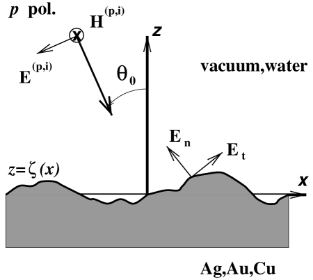
FIG. 1.: Schematic of the scattering geometry with the electromagnetic field vectors for $p$ linear polarization.

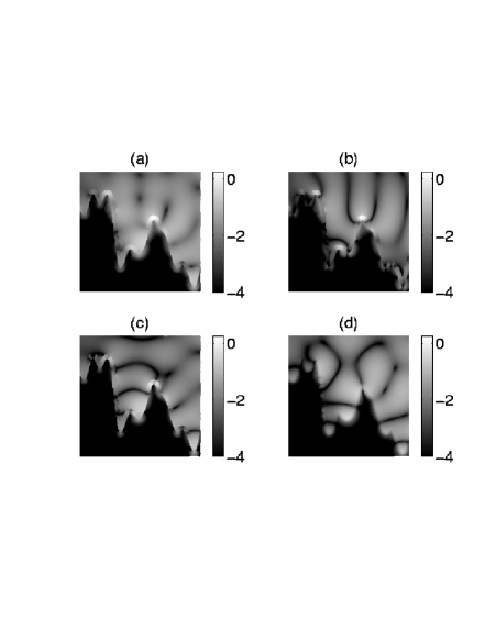
FIG. 2.: Near field intensity images (in a $\log_{10}$ scale) resulting from the $p$-polarized scattering with $\theta_{0}=0^{\circ}$, $\lambda=514.5$ nm, and $W=L/4\cos\theta_{0}$, from a Ag fractal surface with $D=1.9$, $\delta=514.5$ nm, $L=10.29\mu$m, and $N_{p}=2000$. The area shown is 1$\times 1\mu$m². (a) Electric field; (b) Electric field, $z$ component (vertical); (c) Electric field, $x$ component (horizontal); (d) Magnetic field.

FIG. 3.: Surface EM field intensity for the region of the Ag fractal profile (also depicted) shown in Fig. 2. Solid curve: Electric field; dashed curve: Electric field, normal component; long-dashed curve: Electric field, tangential component; dot-dashed curve: Magnetic field. The inset zooms in the largest hot spot.

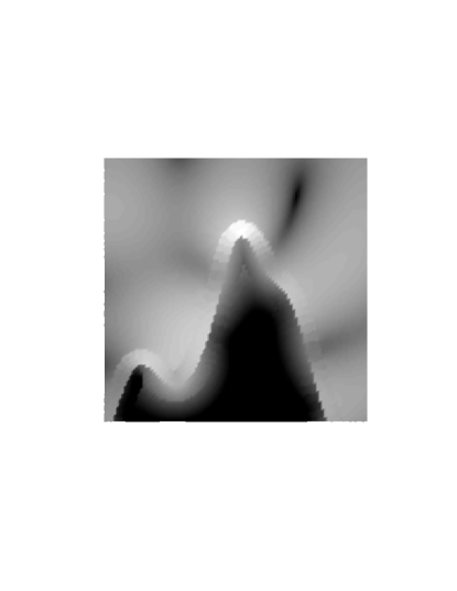
FIG. 4.: Near electric field intensity image (in a $\log_{10}$ scale) for the hot spot area shown in Fig. 2 for a Ag fractal surface with $\theta_{0}=0^{\circ}$, $D=1.9$, $\delta=514.5$ nm, $\lambda=514.5$ nm, $L=10.29\mu$m, $W=L/4\cos\theta_{0}$, and $N_{p}=2000$. The area shown is 500$\times 500$ nm².

FIG. 5.: Surface electric field intensity at the hot spot shown in Fig. 3 but for additional, slightly shifted incoming wavelengths $\lambda=$476.9, 495.9, 539.1, and 563.6 nm.

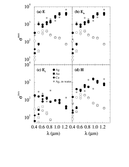
FIG. 6.: Spectral dependence of the maximum local FE $\sigma^{max}$ resulting from the $p$-polarized scattering with $\theta_{0}=0^{\circ},5^{\circ},10^{\circ},\ldots,50^{\circ}$, and $W=L/4\cos\theta_{0}$, from fractal metal surfaces with $D=1.9$, consisting of $N_{r}=60$ realizations of $L=10.29\mu$m and $N_{p}=1600$. (a) Electric field; (b) Electric field, normal component; (c) Electric field, tangential component; (d) Magnetic field. Circles, Ag; Squares, Au; Triangles, Cu. Filled symbols: $\delta=514.5$ nm; Hollow symbols: $\delta=102.9$ nm. Stars: water/Ag, $\delta=514.5$ nm.

FIG. 7.: PDF of the $p$-polarized FE factor $p(\sigma)$ for the electric (including both normal and tangential components) and magnetic fields resulting from the $p$-polarized scattering with $\theta_{0}=0^{\circ},5^{\circ},10^{\circ},\ldots,50^{\circ}$, and $W=L/4\cos\theta_{0}$, from fractal metal surfaces consisting of $N_{r}=60$ realizations of $L=10.29\mu$m and $N_{p}=1600$. Solid curve: $D=1.9$ and $\delta=514.5$ nm; dashed curve: $D=1.9$ and $\delta=102.9$ nm; and dotted curve: $D=1.2$ and $\delta=102.9$ nm. (a) $\lambda=514.5$ nm and (b) $\lambda=1064$ nm.

FIG. 8.: Spectral dependence of the average surface FE $\langle\sigma\rangle$ (excitation spectra) resulting from the $p$-polarized scattering with $\theta_{0}=0^{\circ},5^{\circ},10^{\circ},\ldots,50^{\circ}$, and $W=L/4\cos\theta_{0}$, from fractal metal surfaces with $D=1.9$, consisting of $N_{r}=60$ realizations of $L=10.29\mu$m and $N_{p}=1600$. (a) Electric field; (b) Electric field, normal component; (c) Electric field, tangential component; (d) Magnetic field. Circles, Ag; Squares, Au; Triangles, Cu. Filled symbols: $\delta=514.5$ nm; Hollow symbols: $\delta=102.9$ nm. Stars: water/Ag, $\delta=514.5$ nm.

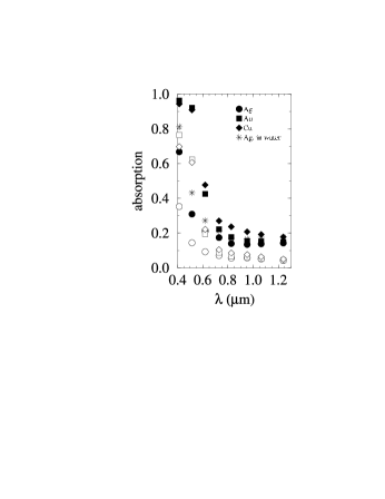
FIG. 9.: Same as in Fig. 8 but for the absorption spectra at normal incidence.

FIG. 10.: Same as in Fig. 8 but for the FE standard deviations $\Delta(\sigma)$.

- [1] S. Nie and S. R. Emory, Science 275, 1102 (1997).
- [2] K. Kneipp, Y. Wang, H. Kneipp, L. T. Perlman, I. Itzkan, R. R. Dasari, and M. S. Feld, Phys. Rev. Lett.78, 1667 (1997).
- [3] K. Kneipp, Y. Wang, H. Kneipp, L. T. Perlman, I. Itzkan, R. R. Dasari, and M. S. Feld, Phys. Rev. Lett.76, 2444 (1996).
- [4] M. Moskovits, Rev. Mod. Phys. 57, 783 (1985).
- [5] A. Wokaun, Molecular Phys. 53, 1 (1985).
- [6] A. Otto, J. Raman Spectrosc. 22, 743 (1991); A. Otto, I. Mrozek, H. Grabhorn, and W. Akemann, J. Phys. Condens. Matter 4, 1143 (1992).
- [7] R. Aroca and G. Kovacs, in Vibrational Spectra and Structure, edited by J. R. Durig (Elsevier, Amsterdam, 1991), Vol. 19, p. 55.
- [8] V. M. Shalaev, Phys. Rep. 272, 61 (1996).
- [9] H. Raether, Surface Polaritons on Smooth and Rough Surfaces and on Gratings (Springer-Verlag, Berlin, 1988).
- [10] D. P. Tsai, J. Kovacs, Z. Wang, M. Moskovits, V. M. Shalaev, J. S. Suh, and R. Botet, Phys. Rev. Lett.72, 4149 (1994).
- [11] S. Bozhevolnyi, B. Vohnsen, I. I. Smolyaninov, and A. V. Zyats, Opt. Commun. 117, 417 (1995); S. Bozhevolnyi, I. I. Smolyaninov, and A. V. Zyats, Phys. Rev. B51, 17 916 (1995).
- [12] P. Zhang, T. L. Haslett, C. Douketis, and M. Moskovits, Phys. Rev. B57 15 513 (1998).
- [13] S. Grésillon, L. Aigouy, A. C. Boccara, J. C. Rivoal, X. Quelin, C. Desmaret, P. Gadenne, V. A. Shubin, A. K. Sarychev, and V. M. Shalaev, Phys. Rev. Lett.82, 4520 (1999).
- [14] R. Jullien and R. Botet, Aggregation and Fractal Aggregates (World Scientific, Singapore, 1987).
- [15] D. Fornasiero and F. Grieser, J. Chem. Phys. 87, 3213 (1987).
- [16] O. Siiman and H. Feilchenfeld, J. Phys. Chem. 92, 453 (1988).
- [17] M. I. Stockman, V. M. Shalaev, M. Moskovits, R. Botet, and T. F. George, Phys. Rev. B46, 2821 (1992).
- [18] S. Sánchez-Cortés, J. V. García-Ramos, and G. Morcillo, J. Colloid Interface Sci. 167, 428 (1994).
- [19] M. C. Chen, S. P. Tsai, M. R. Chen, S. Y. Ou, W.-H. Li, and K. C. Lee, Phys. Rev. B51, 4507 (1995).
- [20] C. Douketis, Z. Wang, T. L. Haslett, and M. Moskovits, Phys. Rev. B51, 11022 (1995).
- [21] A.-L. Barabási and H. E. Stanley, Fractal Concepts in Surface Growth (University Press, Cambridge, 1995).
- [22] M. Xu and M. J. Dignam, J. Chem. Phys. 96, 7758 (1992); 99, 2307 (1993); 100, 197 (1994).
- [23] V. M. Shalaev, R. Botet, J. Mercer, and E. B. Stechel, Phys. Rev. B54, 8235 (1996); E. Y. Poliakov, V. M. Shalaev, V. A. Markel, and R. Botet, Opt. Lett. 21, 1628 (1996).
- [24] E. Y. Poliakov, V. A. Markel, V. M. Shalaev, and R. Botet, Phys. Rev. B57, 14 901 (1998).
- [25] F. J. García-Vidal and J. B. Pendry, Phys. Rev. Lett.77, 1163 (1996).
- [26] J. A. Sánchez-Gil and J. V. García-Ramos, Opt. Commun. 134, 11 (1997).
- [27] J. A. Sánchez-Gil and J. V. García-Ramos, J. Chem. Phys. 108, 317 (1998).
- [28] A. A. Maradudin, T. Michel, A. R. McGurn, and E. R. Méndez, Ann. Phys. NY 203, 255 (1990).
- [29] M. Nieto-Vesperinas, Scattering and Diffraction in Physical Optics (Wiley, New York, 1991).
- [30] J. A. Sánchez-Gil and M. Nieto-Vesperinas, J. Opt. Soc. Am. A 8, 1270 (1991); Phys. Rev. B45, 8623 (1992).
- [31] K. A. O’Donnell, R. Torre, and C. S. West, Opt. Lett. 21, 1738 (1996); M. Leyva-Lucero, E. R. Méndez, T. A. Leskova, A. A. Maradudin, and J. Q. Lu, Opt. Lett. 21, 1809 (1996).
- [32] J. Feder, Fractals (Plenum, New York, 1988).
- [33] R. F. Voss, in: The Science of Fractal Images, edited by H.-O. Peitgen and D. Saupe (Springer, Berlin, 1988); R. F. Voss, Physica D 38, 362 (1989).
- [34] J. A. Sánchez-Gil, J. V. García-Ramos, and E. R. Méndez, to be published.
- [35] A. Mendoza-Suárez and E. R. Méndez, Appl. Opt.36, 3521 (1997).
- [36] D. W. Lynch and W. R. Hunter, in: Handbook of Optical Constants of Solids, edited by E. D. Palik (Academic Press, New York, 1985), p. 356.
- [37] J. A. Sánchez-Gil and A. A. Maradudin, Phys. Rev. B56, 1103 (1997).