Statistical physics of adaptive correlation of agents in a market
Abstract
Recent results and interpretations are presented for the thermal minority game, concentrating on deriving and justifying the fundamental stochastic differential equation for the microdynamics.
Market economics poses several problems of potential interest and challenge to statistical physics, involving the co-operative behaviour of many agents whose actions involve mutual frustration and disorder, both quenched and stochastic. In a nutshell, speculators in an idealized stock market are made up of buyers and sellers, each having personal gain as their objectives, trying to buy low and sell high, making their decisions based on commonly available information using individual strategies, with their collective actions determining the (time-varying) ‘right choices’ and learning from experience. From the point of view of the market regulator, however, preference is for low volatility and market efficiency.
The minority game (MG) is a simple encapsulation of some of the ingredients and issues of a market. It consists of agents each of whom at each step of a parallel dynamical process makes either of two choices, with the objective of being in the minority overall. The agents have no direct knowledge of one another and make their decisions based on purely global information , available equally to all. Their decisions are determined through the application to of individual strategy functions, each agent having a small number of such strategies, drawn randomly and independently from a large distribution at the outset and fixed throughout the game. At each time-step each agent employs (just) one of his or her strategies. Adaptation occurs through the development of functions which determine their choices of strategy.
In the original formulation Challet97 the information was the minority choice over the last time-steps and the adaptation was achieved through the cumulative award of points at each time-step to the strategies which would have yielded the actual minority choice at that step. The strategy played by any agent at any time-step was that of his/her strategies which currently had the largest point-score.
A remarkable observation in simulations Savit99 was that the variance in the minority choice became smaller than that of random choice for large enough , indicating correlation of the agents’ actions. A critical memory length was observed for minimum variance, with agents appearing to be frozen in their choices for , non-frozen for . Moreover, it was shown that the dependence on was through the scaling variable , where was the dimension of the space of strategies Savit99 . Further simulations showed (i) these results are unaffected by replacing the true history by a random Cavagna99 , indicating that as far as macroscopic observables are concerned the ‘information’ merely effectuates the correlation; (ii) replacing the deterministic strategy-choices by stochastic ones can significantly reduce the volatility for information vectors of less than the critical length CGGS99 .
Here we consider the determination of a fundamental analytic theory and report the derivation of the underlying stochastic differential equation for the microdynamics Garrahan00 . We concentrate on a continuous formulation in which is a stochastically randomly chosen unit-length vector on a -dimensional hypersphere, the strategies are quenched random vectors of length in the same space, labeling the agents and the their strategies. The analogues of the binary choices above are bids . The strategies which are actually used are indicated by . The total bid at time is . The point update rule is
| (1) |
For simplicity we specialize to and define
| (2) |
In a generalized thermal minority game (TMG) the probability of strategy use is
| (3) |
and it is useful to define a ‘spin’
| (4) |
In CGGS99 the choice was employed, but here we consider Garrahan00 .
We are interested in coarse-grained average behaviour on a time-scale greater than the step-length in order to pass to a continuum-time theory. Equivalently, we take a time-scale with a differential random noise with zero mean and variance . In the limit a Kramers-Moyal expansion yields Garrahan00
| (5) |
so that to the information noise has been eliminated in favour of an effective interaction between the agents and the averaged variance becomes
| (6) |
where the refer to a temporal average and the bar to an average over the quenched disorder of the strategies.
At Eqs. (2) are deterministic and to leading order in reduce to
| (7) |
| (8) |
| (9) |
At finite temperature correlations between the fluctuations of the right hand sides of Eqs. (5) are of the same order as the mean and Eq. (7) must be replaced by a set of stochastic differential equations Garrahan00
| (10) |
where is the covariance matrix
| (11) |
and is an -dimensional Wiener process of unit scale; for so the Wiener term has no weight. Correspondingly, the Fokker-Planck equation for the probability distribution of the is
| (12) |
The average volatility is given by
| (13) |
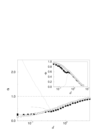
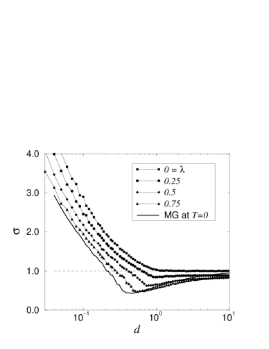
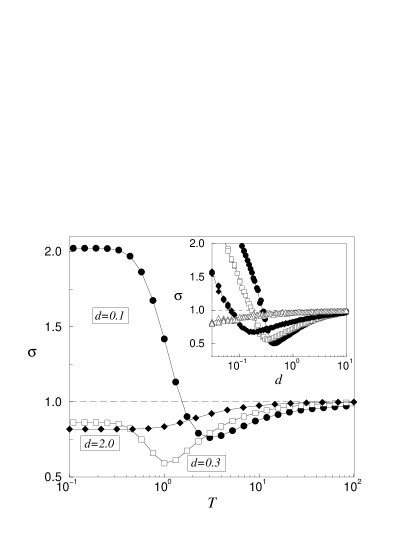
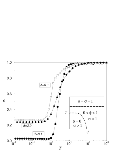
Eq. (10) is thus the fundamental microscopic equation from which the macrodynamics should be calculable. To check this we have compared numerical evaluations of the volatility and the density of frozen agents (those for whom does not change sign after initial transient) from Eqs. (7) and (10) with corresponding direct simulations from Eqs. (1) and (3). They are in perfect accord. This is shown explicitly in Fig. 1 for . Figs. 2a and 2b show the effect of temperature as given by Eq. (10); direct simulation gave results identical within statistical error.
In CMZ00 was evaluated for on the assumption that the system equilibrated and hence was equivalent to minimizing . The result is also exhibited in Fig. 1 and can be seen to be good (and probably correct) for but in error for . In fact, however, Eq. (7) does not describe a simple descent dynamics since the variables on the right and left hand sides are different and a metric is needed to relate and . Substitution shows that the dynamics in non-Markovian in . An explicit demonstration of non-equilibration for follows from a simulation starting with , where is the time-step. This is illustrated in Fig. 3a Garrahan00 .
It is also tempting to compare with a Hopfield neural network which is characterizable by an effective Hamiltonian
| (14) |
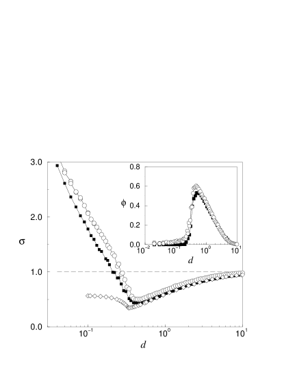
where the are quenched random patterns; indeed it was by the application of techniques devised for (14) that CMZ00 minimized . Clearly there is a difference of sign between Eqs. (8) and (14) but one might be tempted to anticipate that this will merely suppress the retrieval attractors while maintaining the spin glass state, in analogy with the SK model, and then attribute the reduction in energy compared with the random state to spin-glass binding. However, this is false; the Hopfield spin-glass solution is not symmetric under change of sign of . Rather, the random-field term of Eq. (8) is crucial in reducing the ground state energy of and the volatility below their random-state values. This is demonstrated explicitly in Fig. 3b which shows the effect of choosing randomly but as
| (15) |
where is also chosen randomly CMZc00 ; prepa . For and the volatility never falls below random, although again there appears a (different) critical separating regimes (worse-than-random and random).
As noted, above we have used in the simulations. If instead is employed, then for the system iterates over a long time to its zero-temperature behaviour CMZb00 since the mean grows quasi-continuously and saturates to its zero-temperature value, which being eliminates the effects of the second term of Eq. (10). However, for there continues to be an improvement with temperature, to an optimal value which is better than random and is reached at a temperature of CGGS00 , but without any further rise to the random value; in this case fluctuates around .
Finally we remark on the relationship with the crowd-anticrowd concept of HJJH00 , where a crowd is a group of agents playing the same strategy and the corresponding anticrowd play the opposite strategy. From Eq. (6)
| (16) |
where is a unit vector in the Cartesian direction of the D-dimensional space. then formalizes the notion of the number of agents in crowd minus the number in the corresponding anti-crowd. The qualitative difference of and then follows from the recognition that for the vectors are densely distributed on the D-sphere permitting , while for they are sparsely distributed so all .
Acknowledgments
We are grateful to Andrea Cavagna, Irene Giardina and Matteo Marsili for useful comments and discussions. We acknowledge financial support from EPSRC Grant No. GR/M04426 and EC Grant No. ARG/B7-3011/94/27.
References
- (1) Challet, D. and Zhang, Y-C., Physica A 246, 407 (1997).
- (2) Savit, R., Manuca, R. and Riolo, R., Phys. Rev. Lett. 82, 2203 (1999).
- (3) Cavagna, A., Phys. Rev. E 59, R3783 (1999)
- (4) Cavagna, A., Garrahan, J.P., Giardina, I. and Sherrington D., Phys. Rev. Lett. 83, 4429 (1999).
- (5) Garrahan, J.P., Moro, E. and Sherrington, D., Phys. Rev. E85, R9 (2000).
- (6) Challet, D., Marsili, M. and Zecchina, R., Phys. Rev. Lett. 84, 1824 (2000).
- (7) Challet, D. Marsili, M. and Zecchina, R., cond-mat/0004308.
- (8) Cavagna, A., Garrahan, J.P., Giardina, I. and Sherrington, D., cond-mat/0005134.
- (9) Hart, M., Jeffries, P., Johnson, N.F. and Hui, P.M., cond-mat/0003486.
- (10) Challet, D., Marsili, M. and Zhang, Y-C., Physica A 276, 284 (2000).
- (11) Garrahan, J.P., Moro, E. and Sherrington, D., in preparation.