Coexistence of Superconductivity and Spin Density Wave orderings in the organic superconductor (TMTSF)₂PF₆

Abstract

The phase diagram of the organic superconductor (TMTSF)₂PF₆ has been revisited using transport measurements with an improved control of the applied pressure. We have found a 0.8 kbar wide pressure domain below the critical point (9.43 kbar, 1.2 K) for the stabilisation of the superconducting ground state featuring a coexistence regime between spin density wave (SDW) and superconductivity (SC). The inhomogeneous character of the said pressure domain is supported by the analysis of the resistivity between $T_{\text{SDW}}$ and $T_{\text{SC}}$ and the superconducting critical current. The onset temperature $T_{\text{SC}}$ is practically constant ($1.20\pm 0.01$ K) in this region where only the SC/SDW domain proportion below $T_{\text{SC}}$ is increasing under pressure. An homogeneous superconducting state is recovered above the critical pressure with $T_{\text{SC}}$ falling at increasing pressure. We propose a model comparing the free energy of a phase exhibiting a segregation between SDW and SC domains and the free energy of homogeneous phases which explains fairly well our experimental findings.

1 Introduction

The question of competition between a magnetic state and a superconducting (or even only metallic) state is one of the key actual features in the domain of strongly correlated electrons. This point is extensively studied in lamellar superconductors such as the high-T_c copper oxide superconductors orenstein00 and heavy fermion compounds mathur98 . Such a competition is also common in organic materials and an antiferromagnetism(AF)-superconductivity(SC) coexistence region has been observed recently in the $\kappa$-(BEDT-TTF)₂X compounds under well controlled pressure lefebvre00 ; Ito96 . An even better characterised systems featuring the competition of AF(or SDW) and metal or superconductivity is formed by the quasi-one dimensional organic superconductors of the (TM)₂X family, i.e. the Bechgaard-Fabre salts. Even after 25 years of investigation this competition and the exact transition from magnetism to superconductivity remains unclear jerome91 ; ishiguro98 ; bourbonnais99 ; bourbonnais99a . In particular, the prototype and most studied compound, (TMTSF)₂PF₆, has an ideal position in the pressure-temperature phase diagram and an improved experimental setup allows now for investigation of this transition.

In the framework of the Fermi liquid picture, which is expected to be valid in this low temperature part of the phase diagram, it is well known that the formation of a SDW phase in the Bechgaard salts is due to a large Kohn anomaly, associated to an almost perfect nesting of the metallic Fermi surface. When a pressure is applied, the nesting properties are spoiled, which causes a decrease of the ordering temperature $T_{\text{SDW}}$, up to a critical pressure $p_{c},$ at which $T_{\text{SDW}}$ vanishes as observed in the title compound where $T_{\text{S}DW}=12$ K at ambient pressure and becomes a superconductor under high pressures with a critical temperature in the Kelvin range jerome80 . However, it has been noticed in the first experimental reproduction of organic superconductivity under pressure greene80 that both SC and a metal-insulator transition appear to coexist in a narrow pressure domain upon cooling. Such investigation of the phase diagram of the parent compound (TMTSF)₂AsF₆ by Brusetti et al. brus82 has led to similar observations. Then we may add that such competition is also observed in (TMTSF)₂ClO₄ tomic82 where anion disorder is now the driving parameter. Using EPR at low field with helium gas pressure techniques in (TMTSF)₂PF₆ under pressure, Azevedo et al. azevedo84 have reported the existence of a transition between a SDW phase and a superconducting one on cooling in a narrow pressure domain (5.5-5.7 kbar). However, they claimed to be able to rule out the possibility that some parts of the sample are in the SDW state and other in the superconducting state.

On a theoretical point of view, the merging of SDW into the SC state around a critical pressure has been extensively studied. The precursor work of Schulz et al. schulz81 studying the border between SDW and SC states in (TMTSF)₂PF₆ has suggested two possible scenarios, namely, the existence of a quantum critical point between SDW and SC or a first order transition line between the insulating and superconducting states. On the other hand, it is well known that, at a pressure lower than the critical pressure, but close to it, a “semi-metallic” SDW phase is formed, with small pockets of unpaired charge carriers, because the SDW gap is not opened on the whole Fermi surfaceYamaji0 . In some sense, there is a coexistence of metallic and magnetic phases coming from different parts of the reciprocal space. The possibility of a microscopic coexistence of superconducting and SDW phases, at lower temperature, has been studied in detailsYamaji2 , Hasegawa , Yamaji3 . The conclusion was negative, because the density of states of the unpaired carrier pockets, left by the SDW ordering, is strongly reduced compared to that of the metallic phase. Such a reduction drastically decreases the effective superconducting coupling $gN\left(0\right)$, leading to an exponentially small critical temperature.For the sake of completeness we can recall that Machida has proposed a model of microscopically competing orders coming from the different parts of the Fermi surface leading in turn to a coexistence of both orders at low temperature Machida81 .

In this article, using an optimised pressure control, we reinvestigate the critical region of the phase diagram of (TMTSF)₂PF₆, which features the phase boundary between the spin density wave and the superconducting state. Studying the temperature dependence of the resistance and the superconducting critical current, we can obtain some evidence for the existence of an inhomogeneous phase forming in the vicinity of the border. We also propose a simple model which demonstrates that a phase segregation SDW/SC, with formation of macroscopic domains, is always favourable compared to the homogeneous phases.

2 Experimental

We worked with a nominally pure (TMTSF)₂PF₆ single crystal originating from the same batch of high quality crystals used in a previous study vuletic01 . The crystal had standard needle shape and dimensions $3\times 0.2\times 0.1\;mm^{3}$.The four annular contact geometry was used: gold was evaporated on the sample and the leads were attached with silver paste. The contact resistances were just 2-3 Ohms. The high quality of the crystal was confirmed by the resistivity ratio ($\rho_{300K}/\rho_{T_{\text{S}DW}}$) of the order of 1000. All electrical measurements were performed along the needle a-axis. Linear resistance measurements were performed using a standard AC low frequency technique. High critical currents measurements were performed using a DC pulsed technique described elsewhere vuletic01 with 10 $\mu$s short pulses and amplitudes up to 100 mA. The pulse repetition period was 40 ms, i.e. 4000 times longer than the pulse. This is enough to avoid Joule heating of the sample even at the highest amplitudes of 100 mA. Non-heating was also checked by the shape of the pulse displayed on the osciloscope. If heating effects were present at the highest currents (0.3, 1 mA) then the SDW resistance just above $T_{sc}$ should get lower at increasing current. Of course, as one can find in the Fig.5, there is no difference in resistances measured in the SDW phase using currents from 0.001 to 1 mA.

The pressure cell was then plugged on a Helium3 cryostat capable of reaching 0.35 K.

The pressure was applied in a regular beryllium-copper cell, with silicon oil inside a Teflon cup as the pressure transmitting medium. This liquid does not freeze abruptly but solidifies continuously thus reducing mechanical stresses and pressure shifts which are common effects at the freezing points of other liquids. This allowed numerous thermal cyclings of the same sample without noticeable cracks.

However, the drawback of such a technique is the requirement to change pressure only when the cell is warmed up to room temperature. For an accurate pressure determination, we used an InSb pressure gaugekoncz78 , located inside the cell close to the sample. The informations from the pressure gauge can be also cross-checked by the known phase diagram of (TMTSF)₂PF₆ cha12 . The InSb gauge was calibrated at ambient temperature against a manganine gauge establishing a linear pressure dependence of the resistance at a rate of 2.5%/kbar in the 6–12 kbar range.

The measurements were conducted in 19 consecutive runs, as follows (see Table 1). For all runs, after application of the pressure at room temperature, the cell was then immediately cooled down to 0.35 K. The electrical measurements done, the sample was warmed back to room temperature and a subsequent increase or decrease of pressure was immediately applied before cooling again. The temperature sweep rates in cooling and warming did not exceed $\pm$60 K/h. The change of pressure was checked by the resistance of the InSb gauge: for instance, a 0.8% increase in resistance determined a 300 bar increment in pressure (the simultaneous decrease of the resistance at room temperature was also used as a secondary pressure gauge). Additionally, the pressure coefficient of the InSb resistance measured at ambient temperature was equal to that measured at 6 K. Thus, we confirmed that all pressure steps we made were measured by the InSb gauge with an accuracy of $\pm$30 bar.

Starting in run #1, at a pressure $p_{1}=6.8$ kbar, we were able to sweep a 4 kbar wide region with increments ranging from 300 to 100 bar. From run #1 to run #16, pressure was always increased in this manner except a 1400 bar increment for the last run. Then from run #16 to run #17, we made a large pressure drop of 2350$\pm$50 bar. This value was calculated from the InSb resistance and also later confirmed by the phase diagram of (TMTSF)₂PF₆. That is, the R vs. T curve for this run #17 was almost identical to the curve of the run #10 (both SDW and SC critical temperatures were found identical within experimental errors). Small pressure increments for run #18 and #19 were again performed in the usual manner. This procedure allowed us to investigate the pressure domain 8.65–9.3 kbar with a control of the pressure which could not be achieved in the early studies.

RUN	pressure	$T_{\text{SDW}}$	$T_{\text{SC}}$	$\Delta$	$R_{\infty}$	$c$
	(kbar)	(K)	(K)	(K)	(m$\Omega$)	vol%
1	6.8	7.9		9.38	12.1	0.03
2	7.1	7.1
3	7.3	6.6
4	7.5	6.2
5	7.7	5.9
6	7.85	5.6
7	8.15	5.3		6.35	12.0	0.09
8	8.35	4.7
9	8.45	4.4		5.74	11.30	0.2
10	8.65	3.8	1.18	5.56	10.60	0.3
17	8.65	3.8	1.18
11	8.75	3.5	1.19	5.58	8.772	0.36
18	8.9	2.85	1.21	6.90	2.473	1.25
12	8.95	2.85	1.21	6.70	2.146	1.4
13	9.1	2.45	1.21	6.90	0.320	5
19	9.2	1.8	1.21	6.30	0.0452	17
14	9.3	1.4	1.21	6.80	0.0022	89
15	9.6		1.195
16	11		1.106			100

Table 1: The complete range of pressures applied on the single crystal of (TMTSF)₂PF₆ studied in this work. Number of the run gives the chronological order of the experiment. Observed spin-density wave, $T_{\text{SDW}}$ and superconducting, $T_{\text{SC}}$, transition temperatures are given. The activation energy, $\Delta$, asymptotic resistances, $R_{\infty}$ and the volume proportion $c$ (vol%) of the metallic phase when the sample is in the coexistence regime are obtained from the fits of $R$ vs.  $T$ data to the recalculated Arrhenius law, Eq. 3.

3 Experimental observations

3.1 The metallic state : $T>T_{\text{SDW}}$, $T>T_{\text{SC}}$

In Fig. 1a, we show the resistance vs. temperature below 20 K for a set of characteristic pressures from 6.8 to 9.2 kbar together with the data at 11 kbar where a direct metal-SC transition is observed. The temperature dependence of the resistance in the metallic state (we concentrate on temperatures below 20 K) is quadratic, as expected when the electron scattering is dominated by electron-electron interactionsgorkov96 .

We have noticed a shift of the $R$ vs.  $T$ curves by a temperature independent resistance value after each pressure run, without any change of the actual temperature dependence. The resistance curves are usually shifted 0.1–0.2 m$\Omega$ upwards after each run (see caption of Fig 1a). This effect is most clearly seen in the metallic state below 20 K since the absolute values of the resistance (1–2 m$\Omega$) become then comparable to the offset. An example of this offset is shown in Fig 1a. The two resistance curves are for run #10 and #17, i.e. they were measured at equal pressures, but with 7 runs performed in-between. The behaviour of run#17 can be made equal to the run #10 provided an offset of 2.5 m$\Omega$ is subtracted from the resistance values of the earlier run #10. We tend to relate this effect to an increase of the residual resistance due to the cumulative creation of defects after each temperature cycle. We will show later that such defects are not cracks as they would add junctions in the sample, which will be easy to detect in the superconducting state. The added defects, then, could be of point disorder nature of unknown origin. It should be noted that such phenomenon was previously unreported. Still, it can not be excluded in all previous studies, since this extensive thermal cyclings were not performed before.

However, the metallic state resistance was the only aspect influenced by the extensive thermal cycling of the sample. The values of resistance in the SDW state which are orders of magnitude higher were not influenced by the thermal cycling and we could not notice any influence on the determination of the transition temperatures. Since a plot of the resistance vs. $T^{2}$ (see Fig. 1b) reveals the existence of a quadratic temperature dependence below about 12 K with a residual resistance increasing slightly after each pressure run, we have decided to use the value of the residual resistance obtained in run #1 as the reference value, assuming that the sample was the least damaged in the first run, as compared to all subsequent runs. So doing, we noticed that the resistance is weakly pressure dependent at 20 K and becomes insensitive to pressure below 10 K in the pressure domain investigated.

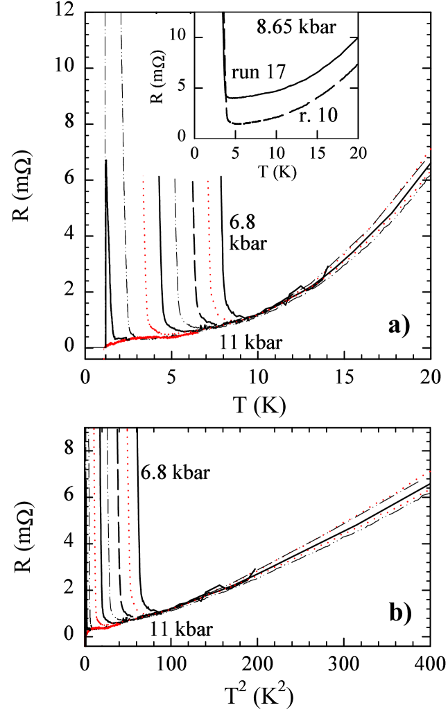
Figure 1: (a) Resistance vs. temperature curves for the usual set of pressures (see legend in Fig. 2), the sharpness of the transitions may be fully appreciated. The behaviour above M - SDW transition is characterised by the unexpected positive pressure coefficient. This is due to the residual resistance, which increases for consecutive pressure runs. In the inset: A detail of the minimum in the $R$ vs.  $T$ curves. For runs 10 and 17, both measured at 8.65 kbar, resistance shift amounted to 2.5 m$\Omega$. (b) Resistance vs. temperature squared curves for the given list of pressures. Low temperature behaviour approaches the $T^{2}$ law of 3D metals.

Figure 2: (a) Logarithm of resistance vs. temperature in cooling, at different pressures. Above the SDW transition (step-like features) the resistance decreases as expected for a metal. (b) $T_{\text{SDW}}$ is defined as the peak in the derivative of logarithm of resistance over inverse temperature, $\partial(\ln R)/\partial(1/T)$ vs. temperature, $T$. Peaks are shown for the pressures denoted in the figure above.

3.2 The SDW regime: $p<8.6$ kbar, $T<T_{\text{SDW}}$

As the SDW regime, we denote the low pressure, low temperature region where the transition to the SDW state is observed as a sharp increase of the resistance (Fig. 2a) without any hysteretic behaviour when sweeping temperature up and down. The exact point of the transition is defined as the temperature of the maximum of the logarithmic derivative of the resistance with respect to the inverse temperature, $\partial(\ln R)/\partial(1/T)$ vs.  $T$. In Fig. 2b, we show these maxima corresponding to the $R$ vs.  $T$ curves above. Activation energy values, $\Delta$, are well defined inside broad temperature spans, especially for the pressures in this regime, 6.8–8.45 kbar (Fig. 3). We note here that the asymptotic resistance at infinite temperature, $R_{\infty}$, remains constant in this pressure range as expected in a standard semiconducting model.

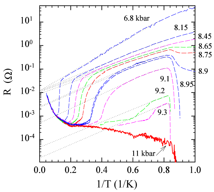
Figure 3: Logarithm of the resistance vs. inverse temperature for the given range of pressures, depicting behaviour in the SDW phase. Fits to the recalculated Arrhenius law (dotted straight lines, Eq. 3) give the same asymptotic resistances, $R_{\infty}$ for the curves inside the pure SDW region. Inside the SDW/M region asymptotic resistances decrease by several orders of magnitude.

3.3 The SC regime: $p>9.43$ kbar, $T<T_{\text{SC}}$

This pressure domain has been briefly investigated at two subsequently applied pressures (9.6 and 11 kbar). A direct transition from a metallic to a superconducting state was observed. $T_{\text{SC}}$ was defined as the onset of the resistance drop. These two pressures differ only in $T_{\text{SC}}$, which are $1.195\pm 0.005$ K and $1.106\pm 0.005$ K respectively. The transitions are very narrow (30-40 mK) and no hysteresis has been observed at $T_{\text{SC}}$. The remaining shift of less than 3 mK observed between cooling and warming curves can be attributed to the finite speed of the temperature sweep, $\pm 1$ mK/s and the thermal inertia of the pressure cell. The mean pressure dependence $\partial T_{\text{SC}}/\partial p\approx-0.07$ K/kbar is in agreement with the value already reported by Schulz et al.  schulz81 .

3.4 The inhomogeneous SDW regime: $8.6<p<9.43$ kbar

We denote as the inhomogeneous regime phase space where both SDW and M (eventually SC) states clearly manifest. Taking advantage of the good pressure control, we managed to investigate eight pressure points with the same sample in this narrow pressure range. They were measured in two groups of five and of three consecutive runs (see Table 1). The second group was measured after a large pressure decrease. This decrease was precisely targeted to reproduce a point (8.65 kbar) in the lower end of the pressure range of interest. This provided a check for our capability of controlling accurately the pressure and an opportunity to investigate in more detail this pressure range in the usual manner by small pressure increments. As already noted, runs #10 and #17 gave almost identical $R$ vs.  $T$ curves except for the residual resistance offset.

3.4.1 $8.6<p<9.43$ kbar, $T_{\text{SC}}<T<T_{\text{SDW}}$: SDW/Metal

As shown in Fig. 4, a strong hysteretic behaviour is observed in this pressure and temperature range between cooling and warming resistance curves leading to the suggestion of an inhomogeneous electronic structure. One possibility is the observation of the famous SDW2 state awaited just below the critical pressure (see the discussion below), but hysteretic behaviour vide-infra is not reasonably compatible with this image. The second possibility is a phase segregation with the existence of metallic domains in a SDW background whose characteristics (size and relative disposition) is strongly temperature dependent.

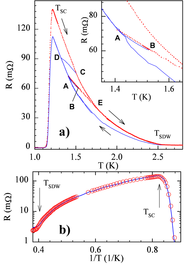
Figure 4: a)Resistance vs. temperature at 9.1 kbar, inside the coexistence range. Solid and dotted lines denote cooling and warming, respectively. The extremal hysteretic loop is recorded when the temperature sweep starts from above $T_{\text{SDW}}$, then cooling continues through points A, D, through $T_{\text{SC}}$, and into superconducting state. Below at least 1 K the sweep may be reversed and warming proceeds through $T_{\text{SC}}$, C, E and back above $T_{\text{SDW}}$ into the SDW phase. Different hysteretic loops appear when temperature sweep is reversed between $T_{\text{SC}}$ and $T_{\text{SDW}}$. Loop 1: cooled from above $T_{\text{SDW}}$ to A, reversed, warmed to E and further to above $T_{\text{SDW}}$. Loop 2: warmed from below $T_{\text{SC}}$ to C, reversed, cooled to D and further to below $T_{\text{SC}}$. Loop 3: cooled from above $T_{\text{SDW}}$ to A, reversed, warmed to B, reversed, warmed to A and further to below $T_{\text{SC}}$. Inset: The position of point B is shown. b) Corresponding $\log R$ vs. $1/T$ plot of normalised extremal curves in cooling (solid line) and in warming (open points).

The extremal hysteretic resistance loop is recorded when the temperature sweep starts above $T_{\text{SDW}}$, reverses below $T_{\text{SC}}$ and ends above $T_{\text{SDW}}$ again. Different hysteretic loops appear when temperature sweep is reversed between $T_{\text{S}C}$ and $T_{\text{S}DW}$ (see Fig.4a for a representative situation at 9.1 kbar). $T_{\text{S}C}$ values determined from either cooling or warming curves are equal (Fig. 4b), within a few mK, as for the direct metal-SC transitions described above. It is quite interesting to note that a highly similar hysteretic behaviour of the thermopower was observed in the CDW state of (NbSe₄)₁₀I₃ Smont92 .

3.4.2 $8.6<p<9.43$ kbar, $T<T_{\text{SC}}$: SDW/SC

In this pressure range, while SDW transitions are still well defined, $R$ vs.  $T$ curves are characterised by a sharp resistance drop at $T=1.2\pm 0.01$ K. We consider this feature to be the manifestation of the condensation of the free-electron domains into superconducting domains. The SC domains either could percolate and form large domains for higher pressures, either, they could link, thanks to sufficiently narrow weak-links allowing for Josephson effect between them at lower pressures. Both mechanisms lead to the zero resistance state.

Initially, at $p=8.65$ kbar, the resistance drops to about 30% of the resistance which would be observed if an Arrhenius behaviour of the SDW state was extended below 1.2 K. This drop is only observed if small (1 to 10 $\mu$A) measuring currents are used. For higher currents (100 $\mu$A), the resistance drop disappears and the usual Arrhenius behaviour is recovered. Then at 8.9 kbar, for the lowest currents, the resistance drops in fact to zero (below our measurable limit of 0.001 m$\Omega$ ). At 8.9 kbar the resistance drop is suppressed concomitantly with the increase of current as shown in Fig. 5. Still, for an current of 1 mA, the resistance drop is far from being completely suppressed (it was not possible to use higher current in order to avoid Joule heating of the sample). Generally, detection of zero resistance at the lowest pressures inside the SDW/SC region requires the lowest measuring current and/or the lowest possible temperatures.

Figure 5: Resistance vs. current at 8.9 kbar. The zero resistance is reached for currents as high as 123 $\mu$A and it was not possible to completely suppress the resistance drop even with a 1 mA measurement current.

As pressure is further increased to 9.1–9.3 kbar, a sharp drop of the resistance to zero within 30–40 mK below the onset temperature is obtained regardless the weak amplitude of the current. In this high pressure regime, we used the pulse technique to determine the critical current, $I_{c}$ without heating effects: at 9.1 kbar, $I_{c}=7$ mA, but at 9.3 kbar, $I_{c}$ raised up to 30–40 mA as shown in Fig. 6. At 11 kbar, the critical current is of the same order of magnitude.

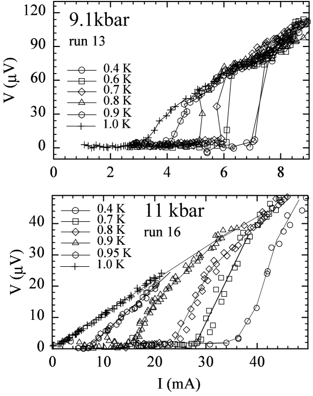
Figure 6: Voltage–current, $V$-$I$ characteristics of the sample at various pressures. (a) At 9.1 kbar, at lowest temperature 0.4 K, the critical current ($I_{c}=7$ mA) is order(s) of magnitude higher than at only 0.2 kbar lower pressure. (b) At 11 kbar the SC state is considered to be homogeneous and $I_{c}$ reaches the maximum value of 40mA.

4 Discussion

4.1 Detailed $p,T$ phase diagram of (TMTSF)₂PF₆

An accurate determination of both transition temperature and pressure enables us to provide a precise $T_{\text{SDW}}$ vs. pressure line, up to the critical point ($p_{c}$=9.43 kbar, 1.2 K) where the suppression of the SDW instability occurs and the SC phase is fully established. That is, for all runs below $p_{c}$, we have observed well defined and narrow metal-SDW transitions. For pressures close to the critical point, the transitions are becoming broader as reported in references brus82 and biskup95 . However, thanks to the good quality of our sample, this effect did not prevent the determination of the transition temperatures even at pressures close to the critical point. This is a salient result of this work because Brusetti et al.  brus82 and Biškup et al.  biskup95 claimed that the SDW transition broadens with pressure approaching the critical pressure. Consequently, they were unable to perform an accurate study of the $T_{\text{SDW}}$ vs. pressure phase boundary at pressures close to $p_{c}$.

Our data combined with the study of Biškup et al. which have determined normal state-to-SDW transition temperatures in the range 1 bar to 7.5 kbar, allow to present a $p,T$ phase diagram of (TMTSF)₂PF₆ displayed in Fig. 7. The fit to an empirical formula which takes into account the fact that $p_{c}$ is found at $T_{\text{SC}}=1.2$ K, and not at $T=0$ K leads to

$$T_{\text{SDW}}(p)=T_{1}-[(T_{1}-T_{\text{SC}})*(p/p_{c})^{3}]$$ (1)

Here $T_{\text{SC}}$ is the experimental value whereas $T_{1}=T_{\text{SDW}}(1bar)$ and $p_{c}$ are free parameters. Best parameter values are $T_{1}=12.0\pm 0.15$ K and $p_{c}=9.43\pm 0.04$ kbar. Obviously, $T_{1}$ and $p_{c}$ values correspond excellently to the experimental ones despite the fact that they were obtained as the only free parameters in the fit. It is also interesting to note that the $T_{\text{SDW}}$ pressure dependence seems to be a pure cubic one.

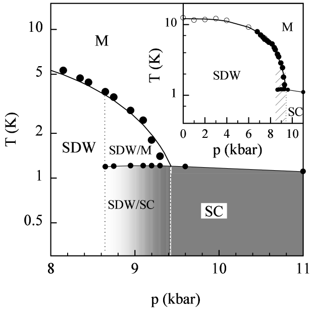
Figure 7: High pressure–low temperature phase diagram of (TMTSF)₂PF₆ material. SDW/M denotes the region where metallic, M, and SDW phases coexist inhomogeneously, below $T_{\text{SDW}}$ line (large full points). Below $T_{\text{S}C}=1.20\pm 0.01$ K line (small full points), this coexistence switches into a coexistence of SC and SDW phases, due to M-SC phase transition. A gradient in shading (SDW/SC region) below $T_{\text{SC}}$ denotes the increase in volume proportion of SC phase in the bulk sample. In inset: Our diagram is completed with data taken from Biškup et al. (open points). Solid curve is the fit to our empirical formula for $T_{\text{SDW}}$ vs. $p$ dependence (Eq. 1).

4.2 Quantification of the domain fraction in the inhomogeneous SDW regime

There are several features in our experimental data substantiating the coexistence of phases, SDW/M above 1.2 K and SDW/SC below 1.2 K. Hysteresis presented in the Fig. 4 is the primary, still only qualitative one. But the other two features (besides evidencing for the coexistence) lead us to the possibility of quantification of the phases volume fraction in the bulk. Indeed, we consider the orders of magnitude change in the critical current, as presented in Figs. 5 and 6 directly proportional to the change in the effective cross-section taken up by superconducting domains for SDW/SC coexistence situation. For the SDW/M situation we intend to show that the change in the effective cross-section taken up by metallic domains may be incurred from the orders of magnitude change in the resistance of the sample for pressures inside the 8.65 – 9.43 kbar region.

In the following we make the assumption that the sample in the inhomogeneous regime behaves as a composite made of two materials. The two materials having the properties of the sample at 11 kbar (pure SC ground state) and 6.8 kbar (pure SDW ground state) respectively.

4.2.1 $T<T_{\text{SC}}$: Quantification of the SDW/SC domain fraction

At 11 kbar, the pressure is sufficiently far above the critical pressure to have a fully homogeneous state, either metallic or SC. Measurements of the critical current from 0.4 to 1.0 K, at this pressure, emphasize this (Fig. 6b). That is, one may divide U/I for the highest currents, which completely suppress SC state, and will recover a resistance which is comparable to the resistances measured above $T_{\text{SC}}$ at this same pressure (values of order of m$\Omega$). Obviously, high currents take the sample from purely superconducting state to a purely metallic state. We conclude then that superconductivity is here homogeneous through the whole cross-section of the sample with a critical current density of $J_{c}=200$ A/cm². Since $T_{\text{SC}}$ is nearly constant in the whole pressure range of the inhomogeneous regime, so should the critical current density.

In the inhomogeneous regime, we can model the sample as alternating insulating (SDW) channels and free electrons (eventually superconducting) channels. For simplicity, the channels are assumed to extend longitudinally from one end of the sample to the other. A change of pressure is equivalent to a change of the cross-section of the metallic (or SC) channels and of the SDW channels. We use the crude approximation that c is temperature independent. In the inhomogeneous regime, in the absence of any weak links along the conducting channels, the SC fraction of the sample cross-section is given by the respective $I_{c}$ value divided by $I_{cMAX}$ measured at 11 kbar, in the pure SC state. Accordingly, at pressures in the inhomogeneous regime, the critical current is lowered, e.g.  at 9.1 kbar, $I_{c}=7$ mA (Fig. 6a). The respective values for other pressures are given in the Table 1.

The resistance recovered for currents above the critical value at 9.1 kbar is only 12 m$\Omega$, i.e.  about 25 times smaller than the resistance of the sample just above $T_{\text{SC}}$ at this same pressure (see Fig. 3). This feature can be ascribed to an electric field overcoming the field required for the depinning of the SDW state. Actually, we calculate the electric field to be of the order of 20 mV/cm at a measuring current of 7 mA ($T=$1 K) using the data for the 9.1 kbar pressure run. This electric field is about four times the value of the depinning field measured in (TMTSF)₂PF₆ tomic91 or (TMTSF)₂AsF₆, traetteberg94 at ambient pressure. The conductance at high currents is therefore the sum of the sliding SDW conductance (which still depends weakly on current) and the conductance of the decondensated free electrons in the suppressed SC, now metallic domains.

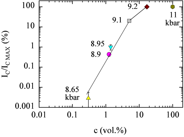
Figure 8: Correlation between the critical current $I_{c}$ (at 0.4 K) and the volume fraction $c$ (vol.%) of the metallic phase in the bulk sample which is present between $T_{\text{SC}}$ and $T_{\text{SDW}}$ in the coexistence regime. Values of both variables are given in Table 1.

4.2.2 $T_{\text{SC}}<T<T_{\text{SDW}}$: Quantification of the SDW/M domain fraction

The principle of additive conductances leads us to a second, independent procedure, for quantification of the SDW/non-SDW domain fraction. We come back to the resistance curves and extract the non-SDW fraction, c, and SDW fraction, 1-c, from the resistance data in the $T_{\text{SC}}<T<T_{\text{SDW}}$ temperature range. Again, we model the sample as alternating insulating (SDW) channels and free electrons (eventually superconducting) channels. Thus, the fraction parameter c is related to effective cross-sections, not the volume of domains. Using this ”rigid model”, the Arrhenius law conductivity can be recalculated as:

$$\sigma(T)=c\sigma_{m}+(1-c)\sigma_{\text{S}DW}$$ (2)

In terms of the resistance we get:

$$1/R(T)=c/R_{m}+(1-c)/R_{\text{S}DW}$$ (3)

where $R_{m}$ is the resistance of a 100% metallic sample and $R_{\text{SDW}}=R_{\infty}exp(\Delta/T)$. Fitting the experimental data $\log R$ vs. $1/T$ to Eq. 3 gave quite good fits as presented in Fig. 3 with the series of dotted lines. The fit parameters c, $\Delta$ and $R_{\infty}$ are given in the Table 1. The observed decrease of $R_{\infty}$ with pressure is the clear demonstration of the increase of the metallic fraction of the sample. The observed evolution of $\Delta$ with pressure is less clear. In pure SDW regime it decreases with pressure, scaled with the transition temperature. Indeed $2\Delta=2.4T_{\text{SDW}}$, although the BCS factor would be 3.52. Further, in the inhomogeneous SDW regime $\Delta$ assumes more or less constant value. We attribute such a result to the fact that the fitting procedure was performed in rather narrow temperature spans, $T_{\text{SC}}<T<T_{\text{SDW}}$.

4.2.3 Correlation of the two quantification procedures

Our study shows that the coexistence regime extends over the 8.65 kbar–9.43 kbar range ($\Delta p=0.78$ kbar). Fig. 8 shows the correlation between the two independent quantifications of the non-SDW fraction c. These were obtained either by critical current measurements in the SC state (y-axis, $I_{cMAX}=$35 mA), or by resistance measurements (x-axis, c from the recalculated Arrhenius law) for $T_{\text{SC}}<T<T_{\text{SDW}}$ range. We therefore plausibly demonstrate the existence of two regimes: a higher inhomogeneous regime (9.1–9.43 kbar) where SC domains extend from one end of the sample to the other, and a lower inhomogeneous regime (8.65–9.1 kbar) where Josephson junctions (or phase slip centers Tinkham ) are present along the conducting channels and further reduce the critical current to lower values.

4.3 The phase segregation scenario

The problem of the metal-insulator transition under pressure has been extensively studied in the context of the canonical Mott transition Mott . The picture proposed by Mott relies on the existence of a first order phase transition between homogenous metallic and insulating phases. According to Mott there exists a critical pressure at which the specific volume jumps discontinuously from its value in the insulating state to the value in the metallic one. The model proposed by Mott did not require a phase segregation regime but only a volume discontinuity from one homogenous state to the other. The situation for (TMTSF)₂PF₆is quite different as experimental data presented above show the existence of a rather broad pressure domain in which the two different orders coexist therefore ruling out the picture of the canonical Mott model. Hence it is the experimental data which have imposed the search of an other approach based on a variational theory leading to an inhomogeneous phase with an energy lower than the energy of homogenous states (SDW or Metal). In the following, we propose a discussion of the experimental data in the framework of the Fermi liquid picture, which is expected to be valid in this low temperature part of the phase diagram. We have to study the relative stabilities of different phases: the metal, the spin density wave, the superconducting phase, but also, of course, possible phases where coexist either a SDW phase and a metallic phase, or, at lower temperature, a SDW phase and a superconducting one.

In order to discuss the stability of the SDW phase, it is therefore essential to model the Fermi surface geometry, i.e. the non interacting electrons dispersion relation. We shall describe the non interacting electron gas by the following two-dimensional dispersion relation :

$$\varepsilon\left(\mathbf{k}\right)=v_{F}\left(\left|k_{x}\right|-k_{F}\right)+t_{\bot}\left(k_{y}b\right)$$ (4)

This dispersion has been linearised around the Fermi level, along the direction $\mathbf{a}$ , corresponding to the highest conductivity, $v_{F}$ is the Fermi velocity and $t_{\bot}\left(k_{y}b\right)$ describes the periodic warping of the Fermi surface along $\mathbf{b}$ the second direction of high conductivity. The third direction, which does not play a major role in this problem, has been ignored. In general, $t_{\bot}\left(k_{y}b\right)$ is responsible for a nearly perfect Fermi surface nesting, which means that there exist a nesting wave vector $\mathbf{Q}$ obeying :

$$\varepsilon\left(\mathbf{k}\right)\simeq-\varepsilon\left(\mathbf{k}+\mathbf{Q}\right)$$

for any wave vector $\mathbf{k}$ of the Fermi surface. The simplest model is given by the following choice GorkovLebed Montambaux2 :

$$t_{\bot}\left(p\right)=-2t_{b}\cos p-2t_{b}^{{}^{\prime}}\cos 2p$$ (5)

For $t_{b}^{{}^{\prime}}=0,$ the Fermi surface is perfectly nested, with wave vector $\mathbf{Q}_{1}=\left(2k_{F},\pi/b\right).\;$Deviations from perfect nesting, which destabilize the SDW phase, are described by a unique parameter $t_{b}^{{}^{\prime}}$. This is an oversimplified description of the Fermi surface geometry, which can be improved by taking into account multiple site transverse transfer integralsYamaji1 . However, we limit, here, our discussion to this simple one-parameter model, which gives the essential physical features. The straightforward extension to a multiple transverse transfer integral model will be given in a forthcoming paper. The critical temperature for the formation of the SDW phase, $T_{\text{SDW}}$ is given by

$$\chi^{0}\left(\mathbf{Q},t_{b}^{{}^{\prime}},T_{\text{S}DW}\right)=1/\lambda$$ (6)

where $\chi^{0}$ is the susceptibility of the non interacting electrons and $\lambda$ is a phenomenological parameter describing the strength of the electron interaction. The wave vector of the magnetic order $\mathbf{Q=}\left(Q_{x},Q_{y}\right)$ should correspond to the maximum of $\chi^{0}\left(\mathbf{Q},t_{b}^{{}^{\prime}},T_{c}\right).\;$In our simple model, we obtain the well known result :

$$\chi^{0}\left(\mathbf{Q},t_{b}^{{}^{\prime}},T\right) = N\left(0\right)\times$$ (7)

$$\times \left[\ln\frac{E_{0}}{T}+\psi(\frac{1}{2})-Re\left\langle\psi(\frac{1}{2}+iB)\right\rangle\right]$$

where $B=A/4\pi T,N\left(0\right)=1/\left(2\pi v_{F}b\right)$ is the density of states at the Fermi level,  $\left\langle\cdots\right\rangle$ means averaging over the transverse momentum $p$, $E_{0}$ is a cutoff proportional to the bandwidth, $\psi$ is the digamma function and :

$$A\left(p\right)=Q_{x}-2k_{F}+\left(1/v_{F}\right)\left[t_{\bot}\left(p\right)+t_{\bot}\left(p-Q_{y}b\right)\right]$$ (8)

Several authorsYamaji2 Hasegawa have considered two different SDW wave vectors. At zero temperature, the best nesting wave vector, denoted $\mathbf{Q}_{2}$ in the literature, connects the inflexion points of the Fermi surface. It is given by :

$$A\left(p,\mathbf{Q}_{2}\right)=\frac{\partial}{\partial p}A\left(p,\mathbf{Q}_{2}\right)=\frac{\partial^{2}}{\partial p^{2}}A\left(p,\mathbf{Q}_{2}\right)=0$$ (9)

At high temperature, when $T$ becomes of the order of $t_{b}^{{}^{\prime}}$ , deviation from perfect nesting becomes irrelevant and the best nesting wave vector is $\mathbf{Q}_{1}=\left(2k_{F},\pi/b\right).\;$According to Hasegawa and FukuyamaHasegawa , $\mathbf{Q}_{2}\left(T\right)$ varies with temperature and jumps to $\mathbf{Q}_{1}$ at a critical temperature $T^{*}=0.232t_{b}^{{}^{\prime}}$ (for $t_{b}/t_{b}^{{}^{\prime}}=20\sqrt{2}$ ). However, as far as we know, no clear experimental evidence of this first order transition has been given.

We first discuss the stability of the homogeneous SDW₁ phase with non varying wave vector $\mathbf{Q}_{1}$. When applying a pressure, the essential feature for this stability is the increase of $t_{b}^{{}^{\prime}}.$ The critical line for the homogeneous order is given by the Stoner criterion (Eq. 6). For a given interaction $\lambda,$ there is a critical line value $t_{b}^{{}^{\prime}*}\left(T\right),$ which means a critical pressure $p_{c}\left(T\right)$ at which the magnetic order disappears. The ratio $T_{SDW}/t_{b}^{{}^{\prime}*},$ where $T_{SDW}$ is the magnetic critical temperature, is a universal function of $\beta=t_{b}^{{}^{\prime}}/t_{b}^{{}^{\prime}*}$ Yamaji2 Hasegawa .

What is revealed, in fact, by the experimental data described above, is the simultaneous formation of two different phases SDW/Metal or SDW/SC, according to the temperature. However, this coexistence corresponds to a segregation in the direct space, not in the reciprocal space. It is quite plausible that such a segregation is not produced on a microscopic scale ($l\ll\xi$ , where $\xi$ is the correlation length) or a mesoscopic scale( $l\sim\xi),$ but rather on a macroscopic scale ( $l\gg\xi$ ), which is much more favorable to the carrier localisation energy necessary to spatially confine the electrons, but also to the interface energy necessary to create domain walls between regions of different orders.

We give very simple and general arguments proving that, near enough to the critical line for the formation of an homogeneous SDW phase, a spatially heterogeneous phase has a lower free energy than the homogeneous SDW phase. The origin of such a phenomenon is due to the following essential physical features :

• The relevant quantity on which depends the SDW order stability is $t_{b}^{{}^{\prime}}$. Applying a pressure increases $t_{b}^{{}^{\prime}}$ and, therefore, the SDW free energy $F_{m}\left(t_{b}^{{}^{\prime}}\right)$, up to a critical value $t_{b}^{{}^{\prime}*}$ at which the homogeneous SDW phase disappears.

• The SDW stability decreases very strongly near $t_{b}^{{}^{\prime}*}.\;$The slope of the critical line is very large.

• The relevant quantity to stabilize the SDW phase near $t_{b}^{{}^{\prime}*}$ is $b,$ the unit cell parameter along the $y-$direction$.\;$Indeed, increasing $b$ strongly decreases $t_{b}^{{}^{\prime}},$ and, therefore, strongly lowers $F_{m}\left(t_{b}^{{}^{\prime}}\right).$

• It is always favorable to create a heterogeneous phase : one part, the volume of which is $\left(1-c\right)\Omega,$ has a cell parameter $b+\delta b_{1}$ and is magnetic, with a lower magnetic free energy because of the lower $b$ parameter ; the other part, the volume of which is $c\Omega$, is metallic and has a cell parameter $b-\delta b_{2}$,($\Omega$ is the total volume), which imposes $\delta b_{2}/\delta b_{1}=\left(1-c\right)/c$. The latter relation implies the constant volume assumption which is considered in the present model (see also Sec.5 for additional arguments). The elastic energy cost for such a deformation is, indeed, proportional to $\left(\delta b\right)^{2}$ and, therefore of second order, while the deformation allows to gain a magnetic free energy proportional to the first order quantity $\left(\frac{\partial F_{m}}{\partial t_{b}^{{}^{\prime}}}\right)\left(\frac{\partial t_{b}^{{}^{\prime}}}{\partial b}\right)\delta b.\;$The larger the slope$\left(\frac{\partial F_{m}}{\partial t_{b}^{{}^{\prime}}}\right),$ the larger the free energy lowering.

The physical picture is clear : near enough to the “homogeneous critical line”, for a pressure lower than the critical pressure, the formation of macroscopic metallic domains or “ribbons”(in this 2D model), with a lower $b$ parameter, parallel to the direction of highest conductivity, allows the formation of SDW “ribbons”, which on the contrary have a larger $b$ parameter. The elastic energy cost is

$$\Delta E_{elastic} = \left(1-c\right)K\left(\delta b_{1}\right)^{2}+cK\left(\delta b_{2}\right)^{2}$$ (10)

$$= \frac{1-c}{c}K\left(\delta b_{1}\right)^{2}$$

where $K$ is an elastic constant. The magnetic free energy lowering, compared to the homogeneous phase free energy, is given by

$$\Delta F_{m}=\left(1-c\right)\left(\frac{\partial F_{m}}{\partial t_{b}^{{}^{\prime}}}\right)\left(\frac{\partial t_{b}^{{}^{\prime}}}{\partial b}\right)\delta b_{1}-cF_{m}\left(t_{b}^{{}^{\prime}}\right)$$ (11)

This linear approximation is quite satisfactory because the derivative is quite large. Minimizing the total free energy $\Delta F_{total}=\Delta E_{elastic}+\Delta F_{m}$ with respect to $\delta b_{1}$ and c , we find that the stable phase is heterogeneous, with a fraction c of metallic phase forming macroscopic metallic domains parallel to $\mathbf{a}$ :

$$c=\frac{1}{2}-\frac{2K\;sgn\left(t_{b}^{{}^{\prime}}-t_{b}^{{}^{\prime}*}\right)\left|F_{m}\left(t_{b}^{{}^{\prime}}\right)\right|}{\left(\frac{\partial F_{m}}{\partial t_{b}^{{}^{\prime}}}\right)^{2}\left(\frac{\partial t_{b}^{{}^{\prime}}}{\partial b}\right)^{2}}$$ (12)

The free energy of the heterogeneous phase is given by

$$\Delta F_{total}=-\frac{1}{4}\frac{\left[\frac{1}{4K}\left(\frac{\partial F_{m}}{\partial t_{b}^{{}^{\prime}}}\right)^{2}\left(\frac{\partial t_{b}^{{}^{\prime}}}{\partial b}\right)^{2}-F_{m}\left(t_{b}^{{}^{\prime}}\right)\right]^{2}}{\frac{1}{4K}\left(\frac{\partial F_{m}}{\partial t_{b}^{{}^{\prime}}}\right)^{2}\left(\frac{\partial t_{b}^{{}^{\prime}}}{\partial b}\right)^{2}}<0$$ (13)

On the “homogeneous critical line”, the fraction of metallic phase is $c=1/2.$ It decreases as $t_{b}^{{}^{\prime}}$ or the applied pressure decreases and vanishes when :

$$\left|F_{m}\left(t_{b}^{{}^{\prime}}=t_{b1}^{{}^{\prime}}\right)\right|=\frac{1}{4K}\left(\frac{\partial F_{m}}{\partial t_{b}^{{}^{\prime}}}\right)^{2}\left(\frac{\partial t_{b}^{{}^{\prime}}}{\partial b}\right)^{2}$$ (14)

which defines $t_{b1}^{{}^{\prime}}$ , the lower critical pressure for the formation of the heterogeneous phase. For $t_{b}^{{}^{\prime}}<t_{b1}^{{}^{\prime}}$ , the stable phase is an homogeneous SDW phase.

In a symmetrical way, for $t_{b}^{{}^{\prime}}$ larger than the critical value, i.e. when the homogeneous phase is metallic, the total free energy is lowered by the formation of SDW macroscopic domains, forming magnetic “ribbons” along the $\mathbf{a}$ direction. An expression quite similar to the case $t_{b}^{{}^{\prime}}<$ $t_{b}^{{}^{\prime}*}$ can be obtained. We find again that $c=1/2$ on the “homogeneous critical line” and increases with $t_{b}^{{}^{\prime}},$ i.e. with the applied pressure and goes to $1$ when :

$$F_{m}\left(t_{b}^{{}^{\prime}}=t_{b2}^{{}^{\prime}}\right)=\frac{1}{4K}\left(\frac{\partial F_{m}}{\partial t_{b}^{{}^{\prime}}}\right)^{2}\left(\frac{\partial t_{b}^{{}^{\prime}}}{\partial b}\right)^{2}$$ (15)

which defines $t_{b2}^{{}^{\prime}}$ , the upper critical pressure for the formation of an heterogeneous phase. For $t_{b}^{{}^{\prime}}>t_{b2}^{{}^{\prime}}$ , the stable phase is an homogeneous metal.

In Fig. 9 we have displayed schematically the pressure dependence of the magnetic condensation energy and the stability domain of the spatially modulated phase with the energy of the inhomogenous phase (continuous line) which is lower than that of the unstable homogenous phase (dashed line).

Figure 9: Schematic behaviour of the energy in the instability domain. The x-axis is $t_{b}^{{}^{\prime}}$ but can be the applied pressure as well.

It should be stressed that we did not take into account the energy necessary to form domain walls between the metallic and magnetic domains. We did not take into account either the energy necessary to localize the carriers within a domain. Since the domains are believed to be macroscopic, the corresponding corrections should be quite small.

Clearly, at lower temperatures, the macroscopic metallic domains should undergoe a transition to a superconducting order, since the phase diagram exhibits a competition between magnetic and superconducting orders. We have, therefore, to investigate the formation of an heterogeneous phase, with coexisting SDW and superconducting domains. Similar calculations can be done by including the superconducting phase free energy, $F_{s},$ which will be assumed to be independent of $t_{b}^{{}^{\prime}}.$ Such an approximation is certainly valid in the narrow pressure range considered here. We shall not make any assumption, neither on the physical mechanism inducing the superconductivity, nor on the symmetry of the order parameter. We shall only suppose that $F_{s}$ is given by the usual mean field expression. As above, we find that the total free energy is lowered by the formation of an heterogeneous phase, on both sides of the “homogeneous critical line”, with a volume $c$ of superconducting domains and a volume $\left(1-c\right)$ of SDW domains. $c$ vanishes for $t_{b}^{{}^{\prime}}\leq$ $t_{b3,}^{{}^{\prime}}$ where the lower critical value $t_{b3}^{{}^{\prime}}$ is given by :

$$-F_{m}\left(t_{b3}^{{}^{\prime}}\right)=\frac{1}{4K}\left(\frac{\partial F_{m}}{\partial t_{b}^{{}^{\prime}}}\right)^{2}\left(\frac{\partial t_{b}^{{}^{\prime}}}{\partial b}\right)^{2}-F_{s}$$ (16)

Since $F_{s}<0,$ the coexistence region gets broader when the superconducting order grows as $T\rightarrow 0.\;$In the same way, in the superconducting region of the homogeneous phase diagram, the total free energy is lowered by the formation of a fraction$\left(1-c\right)$ of SDW domains. On the “homogeneous critical line”, $c=1/2$ and increases when $t_{b}^{{}^{\prime}}$ increases, up to an upper critical value $t_{b4}^{{}^{\prime}}$ , given by ;

$$F_{m}\left(t_{b4}^{{}^{\prime}}\right)=\frac{1}{4K}\left(\frac{\partial F_{m}}{\partial t_{b}^{{}^{\prime}}}\right)^{2}\left(\frac{\partial t_{b}^{{}^{\prime}}}{\partial b}\right)^{2}+F_{s}$$ (17)

In order to calculate explicitly the critical lines, it is necessary to evaluate the magnetic free energy $F_{m}\left(t_{b}^{{}^{\prime}}\right).$ Its expression can be found in the literature. Near the critical line, a Landau expansion can be writtenMontamb40 :

$$F_{m}=\frac{8\pi T_{SDW}^{2}N\left(0\right)}{Re\left\langle\psi"\left(\frac{1}{2}+iB\right)\right\rangle}\left[\frac{\partial\chi^{0}}{\partial T}dT+\frac{\partial\chi^{0}}{\partial t_{b}^{{}^{\prime}}}dt_{b}^{{}^{\prime}}\right]$$ (18)

The quantities $t_{b}^{{}^{\prime}*}\frac{\partial\chi^{0}}{\partial T}$ and $t_{b}^{{}^{\prime}*}\frac{\partial\chi^{0}}{\partial t_{b}^{{}^{\prime}}}$ are well known universal functions of $\beta=t_{b}^{{}^{\prime}}/t_{b}^{{}^{\prime}*},$ given in the literatureMontamb40 ,

$$t_{b}^{{}^{\prime}*}\frac{\partial\chi^{0}}{\partial T} = -N\left(0\right)\frac{t_{b}^{{}^{\prime}*}}{T_{SDW}}\times$$ (19)

$$\times \left[1+Im\left\langle B\psi^{\prime}\left(\frac{1}{2}+iB\right)\right\rangle\right]$$

$$t_{b}^{{}^{\prime}*}\frac{\partial\chi^{0}}{\partial t_{b}^{{}^{\prime}*}} = -N\left(0\right)\frac{t_{b}^{{}^{\prime}*}}{T_{SDW}}\times$$ (20)

$$\times Im\left\langle\pi^{-1}\cos\left(2p\right)\psi^{\prime}\left(\frac{1}{2}+iB\right)\right\rangle$$

where $\psi^{\prime}$ is the trigamma function. These expressions allow a complete determination of $F_{m}$ close to the critical line.

In the limit of vanishing temperature, the magnetic free energy becomes the SDW energy :

$$F_{m}\left(t_{b}^{{}^{\prime}}\right)\rightarrow N\left(0\right)\left[\left(t_{b}^{{}^{\prime}}\right)^{2}-\left(M_{0}\right)^{2}\right]$$ (21)

where $M_{0\text{ }}$is the magnetic order parameter at zero temperature. Expressions (18-21), together with the standard mean field expression for $F_{s}$ allow a complete determination of the critical lines $c=0$ and $c=1$, which give the limits of stability of the heterogeneous phase in the $(T,t_{b}^{{}^{\prime}})$ plane, or, equivalently in the $(T,p)$ plane. A schematic illustration of the theoretical phase diagram is displayed on Fig. 10.

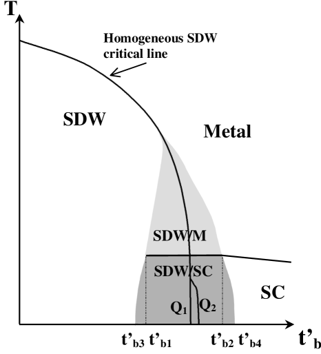
Figure 10: Schematic phase diagram showing the inhomogeneous SDW/M and SDW/SC phases in the vicinity of the critical border. The x-axis can be the applied pressure as well. The heavy lines in the homogenous phase region correspond to $\mathbf{Q}_{1}$ and $\mathbf{Q}_{2}$ SDW states.

We would like to emphasise that, within our model, we do not expect any pressure variation of the superconducting critical temperature $T_{c}$, as experimentally observed, in the heterogeneous phase. It is possible to interpret $T_{c}$ as the ordering temperature of the metallic domains. Nevertheless, we expect the superconducting ordering increases the width of the pressure range in which the heterogeneous phase is stable, because it lowers the total free energy.

The maximum width of the stability region of the heterogeneous phase is obtained at zero temperature. We consider the following numerical values of the parameters entering the model : $E_{0}=3000K,$ $t_{b}^{{}^{\prime}}=10K$ Montambaux2 Montambaux3 , $\frac{\partial t_{b}^{{}^{\prime}}}{\partial p}=1$K/kbar Grant Ducasse , $\frac{1}{b}\frac{\partial b}{\partial p}=3$ $10^{-3}$ kbar^-1these . These values can be considered as typical. We obtain a pressure range of stability of the heterogeneous phase of the order of 1 kbar. The agreement with experiments can be considered as extremely good, if we consider the crudeness of the model.

We discuss now the case of the SDW₂ phase corresponding to the wave vector $\mathbf{Q}_{2}$ Near to the transition between SDW₁ and SDW₂ studied by Hasegawa and FukuyamaHasegawa , a Landau expansion of the magnetic free energy similar to equation (18) can be given, but with different values of $\frac{\partial\chi^{0}}{\partial T}$ and $\frac{\partial\chi^{0}}{\partial t_{b}^{{}^{\prime}}}.$ It is known that the absolute value of the critical line slope is smaller for the SDW₂ phaseMontamb40 Hasegawa . For that reason, the free energy lowering associated to the formation of an heterogeneous phase is larger when the magnetic phase is the SDW₁ phase. We therefore expect that the formation of the heterogeneous phase SDW${}_{1}+$ Metal precludes the formation of the SDW₂ phase, at least near the region of transition between SDW₁ and SDW₂

It is also possible to discuss the stability of the SDW₂ phase in the limit of zero temperature. Hasegawa and FukuyamaHasegawa , as well as YamajiYamaji2 , have studied theoretically the stability of an homogeneous SDW phase. As a result, they predict the stability of an homogeneous SDW₂ phase in a narrow pressure range, for $p$ larger than the critical value $p_{c1}$ at which SDW₁ disappears, but below a second critical pressure $p_{c2.}$ However, in this pressure range, while the magnetic free energy $F_{m}\left(t_{b}^{\prime}\right)$ is slightly lower for the SDW₂ phase, the absolute value of the slope $\left|\frac{\partial F_{m}}{\partial t_{b}^{{}^{\prime}}}\right|$ is much smaller than in the SDW₁ phase and almost vanishes at $p=p_{c2}.$ The lower slope leads to an energy decrease associated to an heterogeneous phase which is lower than in the case of the SDW₁ phase and vanishes as $p\rightarrow p_{c2}$. Using the same model of non interacting Fermi surface as ours, Hasegawa and Fukuyama calculated that the SDW₂ phase is stable up to $t_{b}^{{}^{\prime}}=1.03t_{b}^{{}^{\prime}*}$ Hasegawa , which leads to a pressure range for the SDW₂ stability certainly smaller than 0.3 kbar. Yamaji obtained a similar result for the same Fermi surfaceYamaji4 . If this result is correct, within this pressure range, the heterogeneous phase SDW${}_{1}+$ SC phase ($Het_{1}$ phase) is quite probably more stable than the homogeneous SDW${}_{2}(Hom_{2}$ phase). In such a case, the latter magnetic phase could not be observed, which might explain why no experimental signature of a transition between different magnetic phases has been seen in this part of the phase diagram. However, it should be stressed that Yamaji has studied the stability of the SDW${}_{2\text{ }}$phase using a more realistic Fermi surface model, which seems more favourable to the SDW₂ stabilityYamaji2 . Further work is necessary to determine the relative stability of $Het_{1}$ and $Hom_{2}$ phases, when a realistic Fermi surface is taken into account.

5 Conclusion

In summary, this new visit to the $p,T$ phase diagram of (TMTSF)₂PF₆ enables us to reach a better understanding of the cross-over between SDW and SC ground states. The experimental results suggest that a picture of coexisting SDW and SC macroscopic domains prevails in a narrow pressure domain of $\approx 0.8$ kbar below the critical pressure marking the establishment of an homogeneous SC ground state. In spite of a volume fraction of a SC phase strongly depressed at decreasing pressure in the coexistence regime we could not detect any significant change of $T_{\text{SC}}$.The early claim for the absence of SDW/SC coexistence in the vicinity of the critical pressure azevedo84 based on the observation of an EPR response typical for the superconducting instability, can now be understood by the impossibility of the EPR technique to observe the very broad signal coming from the SDW domains.

We have proposed a very simple model which, on the basis of quite general arguments, leads to the formation of a heterogeneous phase, near the critical line of the homogeneous magnetic phase, on both sides of it, where coexist metallic and magnetic domains and, at lower $T$, magnetic and superconducting domains. This result provides a quite plausible interpretation of the data reported here. Obviously, the same kind of arguments might apply to other competing instabilities. What we are proposing is a variational theory which says that it is possible to find an inhomogenous phase with a free energy which is lower than the energy of the homogenous states (SDW or metal). We took for simplicity the assumption that the total volume of the sample is kept constant. In any variational calculation some constraints are, of course, necessarily imposed on the trial wave functions or trial states. Here, we have choosen, as a variational constraint, the constraint of a constant total volume, for the sake of simplicity. Our variational calculation shows that a state exhibiting a ”coexistence” (or phase segragation) has a lower free energy than the homogenous phase. However, such a free energy lowering is not due to the constraint. If we relax the constraint, the free energy of the inhomogenous state could still decrease and be even more stable than that of the homogenous state. But then, the model should rely very much on the detailed pressure dependence of the SDW condensation energy versus pressure.

As far as organics are concerned, it is interesting to mention that similar phenomena have been reported to arise in the recently discovered superconductor of the TM₂X family, (TMTTF)₂PF₆, under very high pressure wilhelm01 but the extreme pressure conditions of the latter compound made a detailed study impossible. An other situation may be encountered with the coexistence of two possible anion orderings namely (1/2,1/2,1/2) and (0,1/2,1/2) in the salt (TMTSF)₂ReO₄ under pressure detected by x-ray scattering moret86 . We may anticipate that the coexistence domain will also be characterised by a segregation between metallic regions (associated to the (0,1/2,1/2) order) and (1/2,1/2,1/2) anion-ordered insulating regions tomic89 . A coexistence between SDW and SC orders has also been mentioned in this latter compound in the narrow pressure domain $8\pm 0.25$ kbar tomic89 .

Furthermore, an immediate consequence of the existence of magnetic macroscopic domains in the superconducting phase is a large increase of the upper critical field $H_{c2}$ which had been reported long time ago by Greene and Engler in (TMTSF)₂PF₆greene80 and by Brusetti et al. in (TMTSF)₂AsF₆brus82 . Finally, Duprat and Bourbonnais duprat01 have recently performed a calculation of the interference between SDW and SC channels using the formalism of the renormalisation group at temperatures below the 1D cross-over in the presence of strong deviations to the perfect nesting. This calculation shows the possibility of reentrant superconductivity in the neighbourhood of the critical pressure and can explain the deviations of the $\Delta/T_{\text{SDW}}$ ratio from the BCS ratio in the vicinity of the critical pressure due to the non-uniform character of the SDW gap over the Fermi surface (although similar deviations are also obtained, for the same physical reason, in a simple mean field treatment gorkov83 ). Very likely, merging the results of reference duprat01 with the present coexistence model could improve the overall theoretical description.

- (1) J.Orenstein and A.J.Millis. Science, 288:468, 2000.
- (2) N.D.Mathur et al. . Nature, 394:39, 1998.
- (3) S. Lefebvre, P. Wzietek, S. Brown, C. Bourbonnais, D. Jérome, C. Méziere, M. Fourmigué, and P. Batail. Phys. Rev. Lett., 85:5420, 2000.
- (4) H.Ito et al. . J.Phys.Soc.Jpn., 65:2987, 1996.
- (5) D.Jérome. Science, 252:1509, 1991.
- (6) T.Ishiguro, K.Yamaji, and G.Saito. Organic Superconductors. Springer Berlin, 1998.
- (7) C.Bourbonnais and D.Jérome. Advances in Synthetic Metals, page 206. eds. P.Bernier and S.Lefrant and G.Bidan Elsevier, 1999.
- (8) see also C.Bourbonnais and D.Jérome. in cond-mat/9903101.
- (9) D.Jérome, A.Mazaud, M.Ribault, and K.Bechgaard. J.Physique.Lett, 1980.
- (10) R. L. Greene and E. M. Engler. Phys.Rev.Lett., 45:1587, 1980.
- (11) R. Brusetti, M. Ribault, D. Jérome, and K. Bechgaard. J.Physique, 43:801, 1982.
- (12) S.Tomić, D.Jérome, P.Monod, and K.Bechgaard. J.Physique-Lett, 43:L839, 1982.
- (13) L.J.Azevedo, J.E.Schirber, J.M.Williams, M.Beno, and D.Stephens. Phys.Rev.B, 30:1570, 1984.
- (14) H. J. Schulz, D. Jérome, M. Ribault, A. Mazaud, and K. Bechgaard. J.Physique-Lett, 279:L–51, 1981.
- (15) K.Yamaji. J. Phys. Soc. Jpn, 51:2787, 1982.
- (16) K.Yamaji. J Phys.Soc.Jpn, 56:1841, 1987.
- (17) Y Hasegawa and H.Fukuyama. J.Phys.Soc. Jpn, 55:3978, 1986.
- (18) K. Yamaji. J.Phys.Soc.Jpn, 52:1361, 1983.
- (19) K.Machida and T.Matsubara. J.Phys.Soc.Jpn, 50:3231, 1981.
- (20) T. Vuletić, C. Pasquier, P. Auban-Senzier, S. Tomić, D. Jérome, K. Maki, and K. Bechgaard. Eur.Phys.J. B, 21:53, 2001.
- (21) M. Kończykowski, M. Baj, E. Szafarkiewicz, L. Kończewicz, and S. Porowski. High Pressure and Low Temperature Physics, page 523. eds. C. W. Chu and I. A. Woollam Plenum Press New York, 1978.
- (22) P.M.Chaikin. J.Phys.I France, 6:1875, 1996.
- (23) L.P.Gorkov. J.Phys.I France, 6:1697, 1996.
- (24) A.Smontara, K.Biljaković, J.Mazuer, P.Monceau, and F.Lévy. J.Phys.Cond.Matt., 4:3273, 1992.
- (25) N.Biškup, S.Tomić, and D.Jérome. Phys.Rev.B, 51:17972, 1995.
- (26) S.Tomić, J.R.Cooper, W.Kang, D.Jérome, and K.Maki. J.Physique I France, 1:1603, 1991.
- (27) O.Traetteberg et al. . Phys.Rev.B, 49:409, 1994.
- (28) M.Tinkham. Introduction to superconductivity. McGraw-Hill Eds, Chap.11, 1996.
- (29) N.F.Mott. Metal-Insulator Transitions. Taylor and Francis, London,1990.
- (30) L. P. Gor’kov and A. Lebed. J.Physique Lett, 45:433, 1984.
- (31) M Héritier, G. Montambaux, and P. Lederer. J.Physique Lett, 45:943, 1984.
- (32) K.Yamaji. J Phys Soc.Jpn, 55:860, 1986.
- (33) G.Montambaux. Phys.Rev.B, 38:4788, 1988.
- (34) G.Montambaux, M.Héritier, and P.Lederer. J.Phys.Cond.Matt, 19:L293, 1986.
- (35) P.M. Grant. J.Physique C3 France, 44:847, 1983.
- (36) L. Ducasse, M. Abderrabba, J. Hoarau, M. Pesquer, B. Gallois, and J. Gaultier. J. Physique C 19 France, 19:3805, 1986.
- (37) B.Gallois et al. . Mol.Cryst.Liq.Cryst, 148:279, 1987.
- (38) K.Yamaji. J.Phys.Soc.Jpn, 53:2189, 1984.
- (39) H.Wilhelm et al. . Eur.Phys.J. B, 21:175, 2001.
- (40) R.Moret et al. . Phys.Rev.Lett, 57:1915, 1986.
- (41) S.Tomić and D.Jérome. J.Phys.Cond.Matt, 1:4451, 1989.
- (42) R.Duprat and C.Bourbonnais. Eur.Phys.J. B, 21:219, 2001.
- (43) L.P.Gor‘kov and A.G Lebed. J.Physique,Suppl, 44:C3-1531,1983.