Antiferromagnetic Heisenberg model on anisotropic triangular lattice in the presence of magnetic field

Abstract

We use Schwinger boson mean field theory to study the antiferromagnetic spin-1/2 Heisenberg model on an anisotropic triangular lattice in the presence of a uniform external magnetic field. We calculate the field dependence of the spin incommensurability in the ordered spin spiral phase, and compare the results to the recent experiments in Cs₂CuCl₄ by Coldea et al. (Phys. Rev. Lett. 86, 1335 (2001)).

The ground states of two-dimensional (2D) Heisenberg models continue to be of great interest.chakravarty ; auerbach In this paper, we study the antiferromagnetic (AF) Heisenberg model on an anisotropic triangular-lattice in the presence of an external magnetic field along the z-axis,

$$H_{S}=\frac{1}{2}\sum_{i,\delta}J_{\delta}\mathbf{S}_{i}\cdot\mathbf{S}_{i+\delta}-\mu B\sum_{i}\mathbf{S}_{i}^{z}.$$ (1)

In the above equation, the summation runs over all the lattice sites $i$ and their neighboring sites $(i+\delta)$. We consider AF nearest neighbor spin-spin couplings, represented by $J$ and $J^{\prime}$ as shown in Fig. 1, with both $J$ and $J^{\prime}\geq 0$. In the absence of the field, this model is equivalent to a class of models recently considered by a number of authors.Zheng99 ; Merino99 ; Manuel99 ; Chung01 The model includes several well known limiting cases. At $J=0$, it is equivalent to 2D square lattice model, whose ground state is a two-sublattice Néel phase. At $J^{\prime}=0$, it becomes a set of decoupled spin chains. At $J^{\prime}=J$ , it is reduced to the isotropic triangular-lattice model, where the ground state is a three-sublattice antiferromagnet. Experimentally, this model may be relevant to the insulating phase of the layered molecular crystals, $\kappa$-(BEDT-TTF)${}_{2}X$,Mckenzie and $\theta$-(BEDT-TTF)₂ RbZn(SCN)₄,Schmalian Our interest on this model is largely motivated by recent experiments on Cs₂CuCl₄. That system is a quasi 2D $S$ =1/2 frustrated Heisenberg antiferromagnet.Coldea97 Coldea et al.Coldea01 have used the neutron scattering to study the ground state and the dynamics of the system in high magnetic fields. Among the observations, these authors found that the incommensurate wave vector changes as the magnetic field increases, and the spiral spin density wave evolves into a fully saturated state.

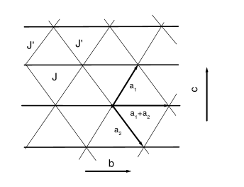
Figure 1: The anisotropic triangle lattice: the bond along the b axis is J and the bond along the a axis is J’.

In this paper we apply the Schwinger boson mean field theory (MFT) to study the effect of magnetic field in the frustrated Heisenberg models. This method enables us to study incommensurate magnetic ordering in the quantum spin systems. The magnetic ordering is identified as the Bose condensation of the Schwinger bosons, and the incommensuration of the ordering is determined by the wave vector of the condensed Schwinger bosons. In the absence of the magnetic field, the MFT predicts three possible ground state: a two-sublattice Neel phase, a spiral spin state, and a spin liquid phase, similar to the results obtained in the high temperature series expansions. Zheng99 In the presence of the field, we calculate the field dependence of the incommensuration in the spiral phase, and compare the results with the experimental observation in Cs₂CuCl₄ with good qualitative agreements.

In terms of Schwinger bosons $a_{i1}$ and $a_{i2}$, the spin operators are expressed as

$$\mathbf{S}_{i}^{+}=a_{i1}^{\dagger}a_{i2};\mathbf{S}_{i}^{-}=a_{i2}^{\dagger}a_{i1};\mathbf{S}_{i}^{z}=\frac{1}{2}(a_{i1}^{\dagger}a_{i1}-a_{i2}^{\dagger}a_{i2})$$ (2)

with a local constraint at every site $i$ given by $a_{i1}^{\dagger}a_{i1}+a_{i2}^{\dagger}a_{i2}=1.$ As a standard method, we introduce a Lagrangian multiplier field $\lambda_{i}$ to describe the constraint. The Hamiltonian of the system then becomes

$$H =-\frac{1}{8}\sum_{i,\delta,\mu,\nu}J_{\delta}A_{ij,\mu\nu}^{\dagger}A_{ij,\mu\nu}-\frac{h}{2}\left(a_{i1}^{\dagger}a_{i1}-a_{i2}^{\dagger}a_{i2}\right)$$

$$+\sum_{i}\lambda_{i}(a_{i1}^{\dagger}a_{i1}+a_{i2}^{\dagger}a_{i2}-1)+\frac{1}{8}\sum_{i,\delta}J_{\delta}$$ (3)

where $h=\mu B;$ $\mu,\nu=1,2$, $j=i+\delta$, and $A_{ij,\mu\nu}=a_{i\mu}a_{j\nu}-a_{i\nu}a_{j\mu}$ is the spin singlet operator of bond $(ij)$. We note that operator $A_{ij,\mu\nu}$ is antisymmetric with respect to either the position $(ij)$ or the indices $(\mu\nu).$ On a bipartite lattice, a spin rotation by $\pi$ on one of the sublattices transforms the spin-singlet bond operators into a symmetric operator with respect to the bond indices $(ij)$. A mean field theory based on that transformation has been developed by Auerbach and Arovas.Auerbach88 The method was extended to study the frustrated lattices by many authors. Yoshioka91 (For an overview of Schwinger boson theory, see Ref. [2] and references therein.) We introduce two types of mean fields: $\Delta_{\mu\nu}(\delta)\equiv\frac{1}{2i}\left\langle A_{jj+\delta,\mu\nu}\right\rangle$ and $\lambda=\left\langle\lambda_{j}\right\rangle$ where $\left\langle\cdots\right\rangle$ represents the thermodynamic average. The mean field Hamiltonian may be solved using the conventional bosonic Bogliubov transformation as well as the Green function’s method.

The mean field Hamiltonian in Eq. (3) is diagonalized as

$$H_{MF}=\sum_{k,\mu=\pm}\omega_{\mu}(k)(\alpha_{k\mu}^{\dagger}\alpha_{k\mu}+\frac{1}{2})+\mathcal{E}_{0},$$ (4)

where the single boson spectra $\omega_{\mu}(k)=\omega(k)\pm h/2$ with $\omega(k)=\sqrt{\lambda^{2}-\left|\gamma(k)\right|^{2}}$ and $\gamma(k)=\sum_{\delta}J_{\delta}\Delta_{12}(\delta)\sin(k\cdot\delta).$ ($\mu=\pm$). $\alpha_{k\mu}$ is a boson annihilation operator related to the original Schwinger bosons. $\mathcal{E}_{0}/N_{\Lambda}=\sum_{\delta,\mu\nu}J_{\delta}(\left|\Delta_{\mu\nu}(\delta)\right|^{2}+1/4)/2-2\lambda.$ The free energy is given by ($\beta=1/k_{B}T$, with $T$ the temperature)

$$F=\frac{1}{\beta}\sum_{k,\mu=\pm}\ln[1-\exp[-\beta\omega_{\mu}(k)]+\frac{1}{2}\sum_{k,\mu=\pm}\omega_{\mu}(k)+\mathcal{E}_{0}.$$ (5)

The mean field Hamiltonian is solved together with the self-consistent equations for the two types of mean fields, which are given by

$$\frac{1}{N_{\Lambda}}\sum_{k,\mu=\pm}\frac{\lambda}{\omega(k)}\left[n_{B}(\omega_{\mu}(k))+1/2\right] =2;$$ (6a)

$$\frac{1}{N_{\Lambda}}\sum_{k,\mu=\pm}\frac{\gamma(k)}{\omega(k)}\sin(k\cdot\delta)\left[n_{B}(\omega_{\mu}(k))+1/2\right] =2\Delta(\delta).$$ (6b)

In the MFT, the magnetic ordering may be identified as the Schwinger boson condensation.Sarker89 Below we examine the possible Schwinger boson condensation at the wave vector $$k=\pm k^{\ast}, \tilde{\omega}_{\mu}(\pm k^{\ast})\rightarrow 0$$ corresponding to the lowest energy of . We introduce a non-negative quantity,

$$b_{0}=\frac{2\lambda}{N_{\Lambda}\omega_{-}(k^{\ast})}\left[n_{B}(\omega_{-}(+k^{\ast}))+n_{B}(\omega_{-}(-k^{\ast}))\right],$$ (7)

such that the points $k=\pm k^{\ast}$ in the integrals in Eqs.(6a) and (6b) are taken into account separately,

$$\sum_{\mu=\pm}\int\frac{dk^{\prime}}{(2\pi)^{2}}\frac{\lambda}{\omega(k)}\left[n_{B}(\omega_{\mu}(k))+1/2\right]$$

$$=2-b_{0};$$ (8a)

$$\sum_{\mu=\pm}\int\frac{dk^{\prime}}{(2\pi)^{2}}\frac{\gamma(k)}{\omega(k)}\sin(k\cdot\delta)\left[n_{B}(\omega_{\mu}(k))+1/2\right]$$

$$=\frac{2J_{\delta}\Delta(\delta)}{J_{\delta}}-b_{0}\gamma(k^{\ast})\sin(k^{\star}\cdot\delta)/\lambda.$$ (8b)

The general features of the mean field solutions in 2D lattices are qualitatively given as below. At any finite $$T b_{0}=0 T=0 \min[\omega(k)]\neq 0 b_{0}=0 \omega(k) \min[\omega(k)]=0 b_{0} Q \omega(k^{\ast})=0$$, . At , if and , the ground state is a spin liquid, whose gap depends on the minimal value of the spectra . If and  is finite, the Schwinger bosons are condensed to the lowest energy state, and the system possesses the magnetic long-range order. The ordering wave vector is determined by . From the spin-spin correlations,

$$\chi_{\alpha\alpha}(q)=-\lim_{\tau\rightarrow 0^{-}}\left\langle T_{\tau}\mathbf{S}_{q}^{\alpha}(\tau)\mathbf{S}_{-q}^{\alpha}(0)\right\rangle\text{ (}\alpha\text{=x,y,z)},$$

we have

$$\chi_{xx}(q) =\chi_{yy}(q)=\chi_{zz}(q)$$

$$=\frac{1}{4N_{\Lambda}}\sum_{k}\left(\frac{n_{B}[\omega(k)]+\frac{1}{2}}{\omega(k)}\right)\left(\frac{n_{B}[\omega(k+q)]+\frac{1}{2}}{\omega(k+q)}\right)$$

$$\times[\lambda^{2}-\gamma(k)\gamma(k+q)]-\frac{1}{16}$$ (9)

for $h=0,$ which indicates the mean field theory does not break SU(2) symmetry. In the thermodynamic limit, ($N_{\Lambda}\rightarrow+\infty$), the correlation functions are convergent except for $Q=2k^{\ast},$

$$\frac{\chi_{\alpha\alpha}(Q)}{N_{\Lambda}}=\frac{b_{0}^{2}}{8}$$ (10)

which indicates that there exists long-range correlations with $Q=2k^{\ast}$ whence $b_{0}\neq 0.$

On the triangular-lattice (see Fig. 1), each site has six neighbors: $\pm\mathbf{a}_{1},\pm\mathbf{a}_{2},\pm(\mathbf{a}_{1}+\mathbf{a}_{2})$. It is convenient to write the wave vector $k=(k_{1},$ $k_{2})$, with $k_{1}$ and $k_{2}$ the components of the vector along the directions of $a_{1}$and $a_{2},$ respectively. The lattice constant $a$ is set to be $1$.

We now consider the mean field solutions at $T=0$. Let me first discuss the solutions in the absence of the field. At $J^{\prime}/J=1$ (the isotropic triangular lattice), $k_{0}^{\ast}=\pi/3$ and $\omega(k^{\ast})=0$, $b_{0}$ is finite indicating a magnetic long range order with the ordering wave vector $Q(2\pi/3,2\pi/3)$. At $J=0$ (the square lattice), $k_{0}^{\ast}=\pi/2$ and $\omega(k^{\ast})=0$, and $b_{0}>0$ implying a Neel ordering at $Q(\pi,\pi)$. The MFT in these two limiting cases is consistent with the known results. At $J^{\prime}=0$ (decoupled one-dimensional chains), the MFT gives $k_{0}^{\ast}=\pi/4$, ($2k^{\ast}$ along the chains), $\omega(k^{\ast})>0$, and $b_{0}=0$, suggesting a spin gap state. The 1D model is exactly soluable, and the ground state is a gapless spin liquid Bethe31 , although the static sin-spin correlation becomes strongest at $Q_{b}=\pi$. Shen98 . The discrepancy between the MFT and the exact solutions is primarily due to the neglect of the topological term in the MFT. For the general values of $J^{\prime}/J$, the MFT predicts three phases at $h=0$: (1). a spin liquid phase at $J^{\prime}/J<0.136$; (2). a spin spiral state at $0.136<J^{\prime}/J<1.70,$ with the ordering wave vector bewteen $(\pi/2,\pi/2)$ and $(\pi,\pi)$; (3). an antiferromagnet with the ordering wave vector $Q=(\pi,\pi)$ at $J^{\prime}/J>1.70$. We note that the phase diagram of the model was studied previously by using a series expansion technique, linear spin density wave and SP(N) mean field theory etc. Zheng99 ; Manuel99 ; Chung01 ; Yoshioka91 In the method of series expansion, they found a Néel state persisting down to $J^{\prime}/J>1.43$, and predicts a spiral phase at small ratio of $J^{\prime}/J$. These are consistent with our MFT. These authors also found a dimer phase between the Néel and spiral states. The dimer phase breaks translational invariance and is not included in the present MFT.

We now consider the soltuions at $h\neq 0$. In this case, the SU(2) rotational symmetry is broken, and $\omega_{-}(k)<\omega_{+}(k)$. The Bose condensation criterion is given by $\omega_{-}(k^{\ast})=\omega(k^{\ast})-h/2=0.$ We use the MFT to study the field dependent incommensurability in the spin spiral phase. The results are shown in Fig. 2, where the vector $k^{\ast}$ are plotted as a function of $J^{\prime}/J$ at several values of $h$. The main feature is as follows. 1) $J^{\prime}/J=1$ is a stable fixed point, around which the external magnetic field does not change the ordering wave vector; 2) At $0.136<J^{\prime}/J<1$, the ordering wave vector increases slightly as the field increases; 3) At $J^{\prime}/J>1$, the ordering wave vector decreases as the field increases; 4) At $J^{\prime}/J<0.136,$ the spin liquid may evolve into a spiral state, and becomes fully saturated as the field further increases.

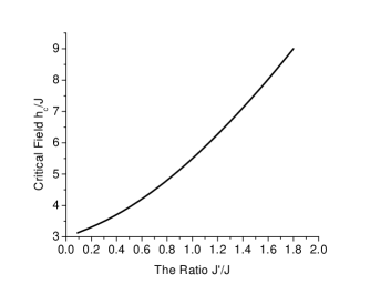
Figure 2: The critical field in unit J versus the ratio $J^{\prime}/J.$

In the presence of the magnetic field, the spin z-component $<S_{z}>\neq 0$, and the ground state breaks the SU(2) invariance. At $T=0$, the expectation value of $S_{z}$ is given by

$$\left\langle\mathbf{S}_{i}^{z}\right\rangle=\frac{1}{2}h^{\ast}b_{0}(k^{\ast},h^{\ast}),$$ (11)

where $h^{\ast}=h/\left(2\lambda\right)$ is the dimensionless field. At $h\neq 0$, $\left\langle\mathbf{S}_{i}^{z}\right\rangle$ is finite, which indicates a polarized component along the field orientation z-axis. The static transverse susceptibilities at $Q=2k^{\ast}$ are given by

$$\frac{\chi_{\alpha\alpha}(Q)}{N_{\Lambda}}=\frac{b_{0}^{2}(k^{\ast},h^{\ast})}{8}\left[1-\left(h^{\ast}\right)^{2}\right]$$ (12)

for $\alpha=x$ and $y$. $\chi_{\alpha\alpha}(Q)/N_{\Lambda}$ decreases as the field increases, and approaches to zero at $h^{\ast}=1$. $b_{0}(k^{\ast},h^{\ast})$ can be calculated within the MFT. A special case is $b_{0}(k^{\ast},h^{\ast}=1)=1$ corresponding to $\left\langle\mathbf{S}_{i}^{z}\right\rangle=1/2$, or the spin full polarization. We have calculated the critical field $\mu B_{c}$ (defined as the lowest field to induce the full spin polarization) as a function of $J^{\prime}/J$. The results are plotted in Fig. 3. As we can see, $\mu B_{c}$ increases as $J^{\prime}$ increases for the fixed $J$. As $J^{\prime}$ increases, the spin couplings are strengthened, and it requires a higher field to polarize the spin.

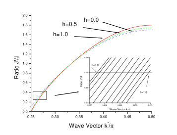
Figure 3: The ratio versus the wave vector $k^{\ast}$ at different fields are ploted. Inset: The wave vector near $J^{\prime}/J=0.33$ at ten different fields are ploted. From left to right, $h^{\ast}=0.0,0.1,\cdots,1.0$.

Very recently, Coldea et al.Coldea01 have reported the neutron scattering experiments on the antiferromagnet Cs₂CuCl₄ in the high magnetic field. That system is a quasi-2D spin-1/2 quantum system in a triangular-lattice as shown in Fig.1. The spin-spin couplings are anisotropic with $J^{\prime}/J\approx 0.33$. In the absence of the external magnetic field, the spins are incommensurately ordered and are aligned within the plane of the triangular-lattice. The latter may indicate a weak deviation from the Heisenberg model. Coldea et al. have studied the low temperature states of the system in the presence of in-plane as well as perperndicular magnetic fields. In the presence of the perpendicular fields, the states are found magnetically ordered with the varying incommensuration below a critical field, above which the system becomes fully spin polarized ferromagnet. In the presence of the in-plane field, they have observed additional spin liquid phase between the incommensurate states and the ferromagnetic phase. There have been theoretical efforts to understand their experimental results.Bocquet01  In the present paper, we have only considered the Heisenberg model in a uniform magnetic field. The predicted spin structure breaks SU(2) symmetry, and shows the spin polarization along the field-direction. Such a spin structure is compatible with the experiments in the perpendicular field, but incompatible with the in-plane field. Therefore, our MFT may be of relevance to the perpendicular field case in their experiments.

Figure 4: The incommensuration $\epsilon$ versus the external field at $J^{\prime}/J=0.33$.

To compare with the experiments, we define a quantity to describe the incommensuration, which is proportional to the wave vector deviation from the Néel state, $\epsilon=1/2-Q_{1}/\pi$, with $Q_{1}$ the component of the spiral wave vector along $a_{1}$ direction. In Table I, we list the experimental Coldea01 and theoretical values of $\epsilon$ at field $h^{\ast}=0$ and at the critical field $h^{\ast}=1$ for the two values of $J^{\prime}/J$. Also listed are the values of $\epsilon$ at $h^{\ast}=0$ calculated from the series expansion method Zheng99 . The agreements between the present MFT and the series expansion at $h^{\ast}=0$ are very good. In Fig. 4, we plot the incommensuration relative to the Néel state as a function of the external field for $J^{\prime}/J=0.33$. Our mean field results are in qualitative agreement with the experiments: as field increases, $\epsilon$ also increases in the parameter space of interest. Quantitatively, the theory predicts a weaker variation in the incommensuration than in the experiments. This discrepancy could be partly due to the neglect of the deviation of the physical system from the Heisenberg model in the theory.

$h^{\ast}$	Exp.Coldea01	$J^{\prime}/J=0.404$	$J^{\prime}/J=0.33$	SEZheng99
$0.0$ ($\epsilon_{0}$)	$0.03$	$0.047$	$0.035$	$0.028$
$1.0$ ($\epsilon_{c}$)	$0.053$	$0.053$	$0.0422$	–

Table I: The incommensuration to the Néel state along the b axis is listed. $h^{\ast}=0$ means the absence the magnetic field, and $h^{\ast}=1$ means the state is saturated fully. SE means the series expansion method, and the data is estimated from the work by Zheng et al.Zheng99 , which was also predicted by Manuel and Ceccatto.Manuel99

In summary, we have used a Schwinger boson mean field theory to study the antiferromagnetic Heisenberg model on an anisotropic triangular lattice in the presence of an external magnetic field. We calculate the magnetic field dependence of the incommensurability of the spin spiral phase. The theoretical results are compared well with the recent neutron scattering experiments.

We would like to thank stimulating discussions with D. A. Tennant and R. Coldea on their experiments. This work was supported by a RGC grant of Hong Kong and a CRCG grant of the University of Hong Kong, and by the US DOE grant No. FG03-01ER45687, and by the Chinese Academy of Sciences. The authors also acknowledge ICTP at Trieste, Italy for its support and hospitality, where part of the work was initiated.

References

- (1) S. Chakravarty, B. I. Halperin, and D. R. Nelson, Phys. Rev. B 39, 2344 (1989).
- (2) A. Auerbach, Interacting Electrons and Quantum Magnetism (Springer-Verlag, New York, 1994).
- (3) Zheng Weihong, R. H. McKenzie, and R. R. P. Singh, Phys. Rev. B 59, 14367 (1999).
- (4) J. Merino, R. H. McKenzie, J. B. Marston, and C. H. Chung, J. Phys.: Condens. Matter 11, 2965 (1999).
- (5) L. O. Manuel and H. A. Ceccatto, Phys. Rev. B60, 9489 (1999).
- (6) C. H. Chung, J. B. Marston, and R. H. Mckenzie, J. Phys. Condens. Mater. 13, 5159 (2001).
- (7) R. H. McKenzie, Comments Condens. Matter Phys. 18, 309 (1998).
- (8) J. Schmalian, Phys. Rev. Lett. 81, 4232 (1998); H. Kino and H. Kontani, J. Phys. Soc. Jpn. 67, 3691 (1998); H. Kino and T. Moriya, J. Phys. Soc. Jpn. 67, 3695 (1998); M. Votja and E. Dagotta, Phys. Rev. B59, 713 (1999).
- (9) R. Coldea, D. A. Tennant, R. A. Cowley, D. F. McMorrow, B. Dorner, and Z. Tylczynski, Phys. Rev. Lett. 79, 151 (1997).
- (10) R. Coldea, D. A. Tennant, A. M. Tsvelik, and Z. Tylczynski, Phys. Rev. Rev. Lett. 86, 1335 (2001).
- (11) A. Auerbach and D. P. Arovas, Phys. Rev. Lett. 61 , 617 (1988); D. P. Arovas and A. Auerbach, Phys. Rev. B 38, 316(1988).
- (12) I. Richey and P. Coleman, J. Phys. Condens. Mater. 2, 9227 (1990); D. Yoshioka and J. Miyazaki, J. Phys. Soc. Jpn. 60, 614 (1991); A. Mattsson, Phys. Rev. B 51, 11574 (1995).
- (13) S. Sarker, C. Jayaprakash, H. R. Krishnamurthy, M. Ma, Phys. Rev. B 40, 5028 (1989).
- (14) H. Bethe, Z. Phys. 71, 205 (1931).
- (15) S. Q. Shen, Inter. J. Mod. Phys. 12, 709 (1998).
- (16) M. Bocquet et al., Phys. Rev. B 64, 094425 (2001).