Thermodynamics and phase behavior of the lamellar Zwanzig model

Abstract

Binary mixtures of lamellar colloids represented by hard platelets are studied within a generalization of the Zwanzig model for rods, whereby the square cuboids can take only three orientations along the $x$, $y$ or $z$ axes. The free energy is calculated within Rosenfeld’s ”Fundamental Measure Theory” (FMT) adapted to the present model. In the one-component limit, the model exhibits the expected isotropic to nematic phase transition, which narrows as the aspect ratio $\zeta=L/D$ ($D$ is the width and $L$ the thickness of the platelets) increases. In the binary case the competition between nematic ordering and depletion-induced segregation leads to rich phase behaviour.

I Introduction

Suspensions of lamellar colloids, like clay dispersions, have received renewed experimental and theoretical attention lately, because of the expected rich phase behaviour, and the obvious geophysical and technological implications, in particular for oil drilling mait:00 . With increasing concentration most natural and synthetic clay dispersions undergo gelation mour:95 which impedes the isotropic to nematic (I-N) transition expected from theoretical considerations onsa:49 and computer simulations eppe:84 ; veer:92 on entropic grounds. It came hence as a relief when a novel system of hard lamellar colloids, namely a dispersion of gibbsite platelets sterically stabilized by a grafted polymer layer, in toluene, was shown to exhibit the expected I-N transition kooi:98 . The difference in behaviour between the gel-forming clays and the novel gibbsite system may lie in the long-range Coulomb interactions present in the aqueous clay dispersions dijk:97 . Subsequently it was shown experimentally kooi:01 , theoretically wens:01 , and by simulation bate:99 , that polydispersity in the size of the platelets strongly affects the phase behaviour. In particular binary mixtures of thin and thick platelets lead to an unexpected isotropic-nematic density inversion kooi:01 ; wens:01 . Moreover, even for monodisperse systems, the phase diagram was shown to be quantitatively, and even qualitatively, sensitive to the aspect ratio (i.e., the thickness over diameter of platelets modeled as ”cut spheres”) veer:92 .

In this paper we address the problem of the phase behaviour of monodisperse and bidisperse systems of hard platelets using a highly simplified model introduced some time ago by Zwanzig to study the I-N transition in systems of hard rods zwan:63 . In this model platelets or rods are represented by square parallelepipeds (or cuboids) of thickness (length) $L$ and width $D$, which can take only three orientations, along the $x$, $y$ or $z$ directions, rather than a continuous range of orientations in space (cf. Fig. 1). The aspect ratio $\zeta=L/D>1$ for rods, while $\zeta<1$ for platelets. The case $\zeta=1$ corresponds to a system of parallel cubes, for which analytic expressions of the first seven virial coefficients are known zwan:56 . Zwanzig’s model may be considered as a highly coarse-grained version of the Onsager long-rod system with continuously varying orientation. The advantage is that virial coefficients beyond the second coefficient $B_{2}$ can be calculated in the limit $\zeta\gg 1$ thus providing a quantitative test of Onsager’s classical theory, which includes only $B_{2}$ onsa:49 . In this paper we adapt Zwanzig’s model to the platelet case ($\zeta<1$) to investigate the equation of state, the I-N transition, as well as binary mixtures of platelets of different size in the search of a possible, depletion-driven demixing transition rowa:02 .

II Model and virial expansion

Following up on Zwanzig’s original idea for rods, we consider a system of $N$ hard square cuboids, of dimension $D\times D\times L$, as shown in Fig. 1, with $L<D$ ($\zeta<1$).

Figure 1: In the model under consideration platelets are represented by square parallelepipeds of thickness $L$ and width $D$, which can take only three orientations, along the $x$, $y$ or $z$ directions. The number density of the centre of mass of the platelet displayed in the figure is denoted by $\rho_{y}$.

The normals to these platelets are restricted to point along one of the Cartesian axes, and platelets of a given orientation are considered as belonging to one of three “species”; the numbers of platelets belonging to each species are denoted by $N_{x}$, $N_{y}$ and $N_{z}$, with the total number of platelets equal to $N=N_{x}+N_{y}+N_{z}$. $N$ is fixed, but the $N_{\alpha}$ fluctuate due to thermal reorientations of the platelets. The mean numbers of platelets per unit volume will be denoted by $\rho_{\beta}=<N_{\beta}>/V$. In an isotropic phase, $\rho_{x}=\rho_{y}=\rho_{z}=\rho/3$, where $\rho=N/V$.

The virial expansion of the excess free energy per unit volume, in powers of the partial densities $\rho_{\beta}$, is:

$$f^{ex}(\{\rho_{\beta}\})=\frac{F^{ex}}{Vk_{B}T}=\sum\limits_{i=2}^{\infty}\frac{1}{i-1}B_{i}(\beta_{1},...,\beta_{i})\rho_{\beta_{1}}\cdot\cdot\cdot\rho_{\beta_{i}}\,,$$ (1)

where the indices $\beta_{1}$, $\beta_{2}$, … sum over $x$, $y$, and $z$. $B_{2}(\beta_{1},\beta_{2})$ is the second virial coefficient between platelets of species $\beta_{1}$ and $\beta_{2}$:

$$B_{2}(\beta_{1},\beta_{2})=-\frac{1}{2}\int d{\bf r}\,f_{\beta_{1},\beta_{2}}({\bf r})$$ (2)

where for cuboids, the Mayer functions reduce to products of Heaviside step functions:

$$f_{\beta_{1},\beta_{2}}({\bf r}) = -\prod_{\alpha=1}^{3}\Theta\left(\frac{1}{2}\left(S_{\alpha,\beta_{1}}+S_{\alpha,\beta_{2}}\right)-|r_{\alpha}|\right)\,.$$ (3)

In Eq. (3), $S_{\alpha,\beta}$ is the spatial extent of plates of species (orientation) $\beta$ in the direction $\alpha=x,y,z$:

$$S_{\alpha,\beta}=D+(L-D)\delta_{\alpha,\beta}\,,$$ (4)

while $|r_{\alpha}|$ is the absolute value of the $\alpha$-component of the vector ${\bf r}_{\alpha}$. For obvious symmetry reasons, there are only two independent $B_{2}(\beta_{1},\beta_{2})$, namely $B_{2}(x,x)=B_{2}(y,y)=B_{2}(z,z)$ (parallel platelets) and $B_{2}(x,y)=B_{2}(x,z)=B_{2}(y,z)$ (orthogonal platelets). The corresponding integrals (2) are easily calculated, to yield:

$$B_{2}(x,x)=4LD^{2}\,;\hskip 5.69046ptB_{2}(x,y)=D(L+D)^{2}\,.$$ (5)

Similarly, there are 3 independent third virial coefficients, namely $B_{3}(x,x,x)$, $B_{3}(x,x,y)$ and $B_{3}(x,y,z)$. These are calculated in Appendix A, together with independent fourth virial coefficients (the latter only in the limits $L\to 0$, $D\to 0$, and $D=L$). Gathering results, the reduced excess free energy density may be cast in the form:

$$f^{ex}=$$ (6)

$$B_{2}(x,x)\left(\rho_{x}^{2}+\rho_{y}^{2}+\rho_{z}^{2}\right)$$

$$+B_{2}(x,y)\left(\rho_{x}\rho_{y}+\rho_{x}\rho_{z}+\rho_{y}\rho_{z}\right)$$

$$+\frac{1}{2}B_{3}(x,x,x)\left(\rho_{x}^{3}+\rho_{y}^{3}+\rho_{z}^{3}\right)+\frac{1}{2}B_{3}(x,y,z)\rho_{x}\rho_{y}\rho_{z}$$

$$+\frac{1}{2}B_{3}(x,x,y)\left[\rho_{x}^{2}(\rho_{y}+\rho_{z})+\rho_{y}^{2}(\rho_{x}+\rho_{z})+\rho_{z}^{2}(\rho_{x}+\rho_{y})\right]$$

$$+O(\rho^{4})\,,$$

and the resulting equation of state reads:

$$\frac{P}{k_{B}T}=$$ (7)

$$\rho+B_{2}(x,x)\left(\rho_{x}^{2}+\rho_{y}^{2}+\rho_{z}^{2}\right)$$

$$+B_{2}(x,y)\left(\rho_{x}\rho_{y}+\rho_{x}\rho_{z}+\rho_{y}\rho_{z}\right)$$

$$+B_{3}(x,x,x)\left(\rho_{x}^{3}+\rho_{y}^{3}+\rho_{z}^{3}\right)+B_{3}(x,y,z)\rho_{x}\rho_{y}\rho_{z}$$

$$+B_{3}(x,x,y)\left[\rho_{x}^{2}(\rho_{y}+\rho_{z})+\rho_{y}^{2}(\rho_{x}+\rho_{z})+\rho_{z}^{2}(\rho_{x}+\rho_{y})\right]$$

$$+O(\rho^{4})\,.$$

It is instructive to consider the isotropic (low density) phase first, where $\rho_{x}=\rho_{y}=\rho_{z}=\rho/3$. Introducing the total (or orientation-averaged) virial coefficients:

$$B_{2} = \frac{1}{3}\left[B_{2}(x,x)+2B_{2}(x,y)\right]\,,$$ (8)

$$B_{3} = \frac{1}{9}\left[B_{3}(x,x,x)+6B_{3}(x,x,y)+2B_{3}(x,y,z)\right]\,,$$ (9)

the equation of state of the isotropic phase reduces to the usual form:

$$\frac{P}{k_{B}T}=\rho+B_{2}\rho^{2}+B_{3}\rho^{3}+O(\rho^{4})\,.$$ (10)

The two important dimensionless parameters in the problem are the size ratio $\zeta=L/D$, and the reduced density (or packing fraction) $\rho^{\star}=\rho D^{2}L$. Substituting the results from Appendix A, the dimensionless equation of state $P/(k_{B}T\rho)$ may be expressed in terms of these two variables as:

$$\frac{P}{k_{B}T\rho}=1+\frac{2}{3}\left(\frac{1}{\zeta}+4+\zeta\right)\rho^{\star}$$

$$+\frac{1}{27}\left(\frac{2}{\zeta^{2}}+\frac{48}{\zeta}+141+52\zeta\right)\rho^{\star 2}+O(\rho^{\star 3})\,.$$ (11)

It is worthwhile to examine three limiting cases, including contributions up to the fourth virial coefficient.

a) Long rods, corresponding to the limit $\zeta\to\infty$; in that case the relevant variable is the Onsager parameter, or effective packing fraction $\eta=\rho^{\star}\zeta=\rho DL^{2}$, in terms of which:

$$\frac{P^{(\rm rods)}}{k_{B}T\rho} = 1+\frac{2}{3}\eta-\frac{16}{243}\eta^{3}+O(\eta^{4})\,,$$ (12)

i.e., the third virial contribution $\sim\eta^{2}$ is identically zero, in agreement with Onsager’s conjecture for rods with continuous orientations onsa:49 , and with Zwanzig’s result zwan:63 .

b) Thin platelets, corresponding to the limit $\zeta\to 0$; in that case the relevant variable is the effective packing fraction $\eta=\rho^{\star}/\zeta=\rho D^{3}$,

$$\frac{P^{(\rm platelets)}}{k_{B}T\rho} = 1+\frac{2}{3}\eta+\frac{2}{27}\eta^{2}-\frac{32}{243}\eta^{3}+O(\eta^{4})\,,$$ (13)

In this case the third virial coefficient $B_{3}$ is non-zero, nor is $B_{4}$, in agreement with numerical findings for continuously rotating disc-shaped platelets eppe:84 . At this stage there is no indication of convergence of the virial series at high packing fraction, but some plausibility arguments will be put forward in the following section to justify truncation of the virial series (13) after the $O(\eta^{2})$ (third virial) term for infinitely thin platelets.

c) Parallel cubes, corresponding to $\zeta=1$; the relevant dimensionless variable is the packing fraction $\eta=\rho^{\star}$, and the first few terms in the virial series read zwan:56 :

$$\frac{P^{(\rm cubes)}}{k_{B}T\rho} = 1+4\eta+9\eta^{2}+\frac{34}{3}\eta^{3}+O(\eta^{4})\,.$$ (14)

In Figure 2 the low density equation of state is shown for several aspect ratios $0\leq\zeta\leq 1$, and compared to available simulation data for hard cubes swol:87 and for infinitely thin discs of the same area ($\pi R^{2}=D^{2}$), but, with continuously varying orientations eppe:84 ; dijk:97 . As expected, the pressure increases rapidly with $\zeta$ for any reduced density $\rho D^{3}$. The results for continuously rotating discs and for squares with discrete orientations are surprisingly close.

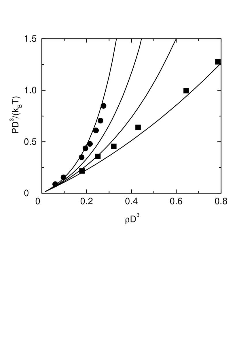
Figure 2: Low density equation of state of a monodisperse, isotropic fluid consisting of rectangular platelets of surface size $D\times D$ and thickness $L$ for various aspect ratios: $\zeta=L/D=0,0.3,0.6,1$ (solid lines from bottom to top). The symbols represent computer simulation data for parallel hard cubes (circles, $D=L$) swol:87 and thin circular platelets (squares, $L\to 0$) eppe:84 ; dijk:97 with continuous allowed orientations.

III Fundamental measure theory for hard platelets

In view of the uncertain convergence of the virial series of the equation of state of hard platelets at high densities ($\eta\geq 1$), it is important to seek an approximate resummation of the series, similar to scaled particle theory for hard spheres reis:59 . This is most conveniently achieved within the framework of Rosenfeld’s FMT rose:88 , by generalizing Cuesta’s work for hard parallel cubes cues:96 to the case of Zwanzig’s model for hard platelets. The second and third virial coefficients calculated in the preceding section provide key input into the theory. Since the free energy of bidisperse platelets will be required to construct complete phase diagrams in section V, the FMT is formulated here for a binary mixture of platelets of size $D_{i}\times D_{i}\times L_{i}$ ($i=1,2$). It is convenient to consider the more general case of inhomogeneous mixtures, characterized by the local densities $\rho^{(i)}_{\beta}({\bf r})$ of the centres of mass of platelets of species $i$, with orientations along $\beta=x,y,z$.

Under the influence of external potentials $V^{(i)}_{\beta}({\bf r})$, the equilibrium density profile of the mixture minimize the grand potential functional:

$$\Omega[\rho^{(i)}_{\beta}({\bf r})] = \sum_{i=1}^{2}\sum_{\beta}\int d{\bf r}\,\rho^{(i)}_{\beta}({\bf r})\left[k_{B}T\left(\ln[\Lambda_{i}^{3}\rho^{(i)}_{\beta}({\bf r})]-1\right)\right.$$ (15)

$$-\left.\mu_{i}+V^{(i)}_{\beta}({\bf r})\right]+F_{ex}[\rho^{(i)}_{\beta}({\bf r})]\,,$$

where the $\mu_{i}$ are the chemical potentials of the two species (irrespective of their orientation), while the $\Lambda_{i}$ are the thermal de Broglie wavelengths. The basic assumption of FMT is to postulate the following form of the excess free energy functional:

$$F_{ex}[\rho^{(i)}_{\beta}({\bf r})]=k_{B}T\int d{\bf r}\,\Phi[n_{l}({\bf r})]\,,$$ (16)

where the reduced excess free energy density $\Phi$ is a function of a set of weighted densities

$$n_{l}({\bf r})=\sum_{i=1}^{2}\sum_{\beta}\int d{\bf r}_{1}\rho^{(i)}_{\beta}({\bf r}_{1})\omega_{l,\beta}^{(i)}({\bf r}-{\bf r}_{1})\,.$$ (17)

The weight functions $\omega_{l,\beta}^{(i)}({\bf r})$ are determined by expressing the Fourier transforms of the Mayer functions $f^{(i,j)}_{\beta_{1},\beta_{2}}$ as sums of products of functions associated with single platelets. In the case of mixtures, equation (3) is generalized as:

$$f^{(i,j)}_{\beta_{1},\beta_{2}}({\bf r}_{1},{\bf r}_{2})=$$ (18)

$$-\prod_{\alpha=1}^{3}\Theta\left(\frac{1}{2}\left(S_{\alpha,\beta_{1}}^{(i)}+S_{\alpha,\beta_{2}}^{(j)}\right)-|r_{\alpha,1}-r_{\alpha,2}|\right)\,,$$

where $S_{\alpha,\beta}^{(i)}=D_{i}+(L_{i}-D_{i})\delta_{\alpha,\beta}$. The Fourier transform of the Mayer function (18) may be decomposed according to:

$$f^{(i,j)}_{\beta_{1},\beta_{2}}({\bf q})=\int\limits^{\infty}_{-\infty}d{\bf r}\,e^{i{\bf q}\cdot{\bf r}}f^{(i,j)}_{\beta_{1},\beta_{2}}({\bf r})$$ (19)

$$= \omega^{(i)}_{0,\beta_{1}}({\bf q})\omega^{(j)}_{3,\beta_{2}}({\bf q})+\omega^{(i)}_{3,\beta_{1}}({\bf q})\omega^{(j)}_{0,\beta_{2}}({\bf q})$$

$$+\mbox{\boldmath$\omega$}^{(i)}_{1,\beta_{1}}({\bf q})\cdot\mbox{\boldmath$\omega$}^{(j)}_{2,\beta_{2}}({\bf q})+\mbox{\boldmath$\omega$}^{(i)}_{2,\beta_{1}}({\bf q})\cdot\mbox{\boldmath$\omega$}^{(j)}_{1,\beta_{2}}({\bf q})\,,$$

where the scalar and vectorial weights ($0\leq l\leq 3$) are defined by:

$$\omega^{(i)}_{0,\beta}({\bf q}) = b^{(i)}_{x,\beta}(q_{x})b^{(i)}_{y,\beta}(q_{y})b^{(i)}_{z,\beta}(q_{z})\,,$$ (20)

$$\mbox{\boldmath$\omega$}^{(i)}_{1,\beta}({\bf q}) = \left(\begin{array}[]{l}a^{(i)}_{x,\beta}(q_{x})b^{(i)}_{y,\beta}(q_{y})b^{(i)}_{z,\beta}(q_{z})\\ \\ b^{(i)}_{x,\beta}(q_{x})a^{(i)}_{y,\beta}(q_{y})b^{(i)}_{z,\beta}(q_{z})\\ \\ b^{(i)}_{x,\beta}(q_{x})b^{(i)}_{y,\beta}(q_{y})a^{(i)}_{z,\beta}(q_{z})\end{array}\right)\,,$$ (26)

$$\mbox{\boldmath$\omega$}^{(i)}_{2,\beta}({\bf q}) = \left(\begin{array}[]{l}b^{(i)}_{x,\beta}(q_{x})a^{(i)}_{y,\beta}(q_{y})a^{(i)}_{z,\beta}(q_{z})\\ \\ a^{(i)}_{x,\beta}(q_{x})b^{(i)}_{y,\beta}(q_{y})a^{(i)}_{z,\beta}(q_{z})\\ \\ a^{(i)}_{x,\beta}(q_{x})a^{(i)}_{y,\beta}(q_{y})b^{(i)}_{z,\beta}(q_{z})\end{array}\right)\,,$$ (32)

$$\omega^{(i)}_{3,\beta}({\bf q}) = a^{(i)}_{x,\beta}(q_{x})a^{(i)}_{y,\beta}(q_{y})a^{(i)}_{z,\beta}(q_{z})\,,$$ (33)

and:

$$a^{(i)}_{\alpha,\beta}(q_{\alpha}) = \frac{2}{q_{\alpha}}\sin\left(\frac{S^{(i)}_{\alpha,\beta}q_{\alpha}}{2}\right)\,,$$ (34)

$$b^{(i)}_{\alpha,\beta}(q_{\alpha})=\cos\left(\frac{S^{(i)}_{\alpha,\beta}q_{\alpha}}{2}\right)\,.$$ (35)

Substitution of the Fourier transforms of the weight functions (20)-(33) into equation (17) yields two scalar and two vectorial weighted densities $n_{l}({\bf r})$. Letting $n_{l}({\bf r})={\bf n}_{l}({\bf r})\cdot{\bf u}$, $l=1,2$, with ${\bf u}=(1,1,1)$, one can construct the function $\Phi$ from the following linear combination of scalar terms, each of dimension (volume)^-1:

$$\Phi[n_{l}({\bf r})]=$$ (36)

$$c_{0}n_{0}({\bf r})+c_{1}n_{1}({\bf r})n_{2}({\bf r})+c_{2}{\bf n}_{1}({\bf r})\cdot{\bf n}_{2}({\bf r})+c_{3}n_{2}^{3}({\bf r})$$

$$+c_{4}n_{2}{\bf n}_{2}({\bf r})\cdot{\bf n}_{2}({\bf r})+c_{5}{\bf n}_{2}({\bf r})\cdot{\bf n}_{2}({\bf r})\cdot{\bf n}_{2}({\bf r})\,,$$

where ${\bf n}\cdot{\bf n}\cdot{\bf n}=n_{x}^{3}+n_{y}^{3}+n_{z}^{3}$. The 6 coefficients $c_{i}$ ($0\leq i\leq 5$) are analytical functions of the only dimensionless weighted density, namely $n_{3}$. These functions are determined, within integration constants, by the scaled particle condition reis:59 , which results in the following differential equation for $\Phi$ rose:88 :

$$-\Phi+\sum\limits_{\beta}\rho_{\beta}\frac{\partial\Phi}{\partial\rho_{\beta}}+n_{0}=\frac{\partial\Phi}{\partial n_{3}}\,.$$ (37)

Substitution of (36) into (37) yields, upon integration:

$$c_{0} = -\ln(1-n_{3})\,,c_{1}=\frac{d_{1}}{1-n_{3}}\,,c_{2}=\frac{d_{2}}{1-n_{3}}\,,$$

$$c_{3} = \frac{d_{3}}{(1-n_{3})^{2}}\,,c_{4}=\frac{d_{4}}{(1-n_{3})^{2}}\,,c_{5}=\frac{d_{5}}{(1-n_{3})^{2}}\,.$$ (38)

The remaining constants $d_{i}$ ($1\leq i\leq 5$) are determined by identifying the low density expansion of the excess free energy, defined by Eqs. (16), (36) and (III) for the homogeneous fluid (i.e., $\rho_{\beta}^{(i)}({\bf r})=\rho_{\beta}^{(i)}$) with the third order virial expansion (1) of the same free energy; this leads to

$$d_{1}=0\,,d_{2}=1\,,d_{3}=\frac{1}{6}\,,d_{4}=-\frac{1}{2}\,,d_{5}=\frac{1}{3}\,.$$ (39)

The final expression for the function $\Phi$ then reads:

$$\Phi=-n_{0}\ln(1-n_{3})+\frac{{\bf n}_{1}\cdot{\bf n}_{2}}{1-n_{3}}+\frac{n_{2,x}n_{2,y}n_{2,z}}{(1-n_{3})^{2}}\,,$$ (40)

where $n_{2,\alpha}$ is the projection of the vector ${\bf n}_{2}$ in the $\alpha$ direction. The FMT expression for the free energy functional is now completely specified. In the limit of parallel hard cubes ($L_{i}=D_{i}$) the excess free energy functional reduces to the result of Ref. cues:96 .

In the limit of a homogeneous bulk fluid the equilibrium density profiles are constant, and the weighted densities take the explicit expressions:

$$n_{0} = \sum_{i=1}^{2}\left(\rho^{(i)}_{x}+\rho^{(i)}_{y}+\rho^{(i)}_{z}\right)\,,$$ (41)

$${\bf n}_{1} = \sum_{i=1}^{2}\left(\begin{array}[]{l}L_{i}\rho^{(i)}_{x}+D_{i}\rho^{(i)}_{y}+D_{i}\rho^{(i)}_{z}\\ \\ D_{i}\rho^{(i)}_{x}+L_{i}\rho^{(i)}_{y}+D_{i}\rho^{(i)}_{z}\\ \\ D_{i}\rho^{(i)}_{x}+D_{i}\rho^{(i)}_{y}+L_{i}\rho^{(i)}_{z}\end{array}\right)\,,$$ (47)

$${\bf n}_{2} = \sum_{i=1}^{2}\left(\begin{array}[]{l}D_{i}\rho^{(i)}_{x}+L_{i}\rho^{(i)}_{y}+L_{i}\rho^{(i)}_{z}\\ \\ L_{i}\rho^{(i)}_{x}+D_{i}\rho^{(i)}_{y}+L_{i}\rho^{(i)}_{z}\\ \\ L_{i}\rho^{(i)}_{x}+L_{i}\rho^{(i)}_{y}+D_{i}\rho^{(i)}_{z}\end{array}\right)D_{i}\,,$$ (53)

$$n_{3} = \sum_{i=1}^{2}L_{i}D_{i}^{2}\left(\rho^{(i)}_{x}+\rho^{(i)}_{y}+\rho^{(i)}_{z}\right)\,,$$ (54)

The weight functions may be interpreted in terms of the following geometric characteristics of the particles: their mean diameter $(L_{i}+2D_{i})/3$, their surface $2D_{i}(D_{i}+2L_{i})$, and their volume $L_{i}D_{i}^{2}$.

In the limit of an isotropic ($\rho_{x}=\rho_{y}=\rho_{z}=\rho/3$) one-component system of platelets, the equation-of-state derived from the free energy density (40) takes the following form (with $\eta=\rho D^{3}$, the effective packing fraction, and $\zeta=L/D$):

$$P^{\star}=\frac{PD^{3}}{k_{B}T} = \eta+\frac{\zeta\eta^{2}}{1-\eta\zeta}+\frac{(2+5\zeta)\eta^{2}}{3(1-\eta\zeta)^{2}}$$ (55)

$$+\frac{2(1+2\zeta)^{3}\eta^{3}}{27(1-\eta\zeta)^{3}}\,.$$

Interestingly, in the $\zeta\to 0$ limit (infinitely thin platelets) the FMT equation-of-state reduces to the virial series (13), truncated after third order. This is reminiscent of the equation of state derived for circular platelets (discs), with continuously varying orientation, from PRISM (polymer reference interaction site model), which also reduces to a three term series (although the coefficients of $\eta^{2}$ and $\eta^{3}$ differ slightly from the exact virial coefficient for that case) harn:01 . These two observations prompt the conjecture that a three term virial series may be quantitatively accurate for infinitely thin platelets (with discrete or continuous orientations) beyond the low density regime.

For finite thickness, however ($\zeta>0$), the three-term virial series and the FMT equation-of-state (55) deviate increasingly as $\zeta$ and $\eta$ increase. Thus, for $\eta=1$, $P^{\star}_{1}$, as calculated from Eq. (II) and $P^{\star}_{2}$, derived from Eq. (55), take the values $P^{\star}_{1}=2.246$ and $P^{\star}_{2}=2.315$ for $\zeta=0.1$, while $P^{\star}_{1}=2.88$ and $P^{\star}_{2}=3.209$ for $\zeta=0.2$; for $\zeta=0.5$, the three-term virial series underestimates the pressure by more than a factor of $2$ ($P^{\star}_{1}=5.676$ and $P^{\star}_{2}=12.74$) for $\eta=1$.

IV Nematic ordering of platelets

As a direct application of the FMT free energy (40) derived in the preceding section, we now consider the possibility of an isotopic to nematic (I-N) transition in a monodisperse fluid of platelets, as a function of the the aspect ratio $\zeta=L/D$. The broken symmetry in the nematic phase may be characterized by the order parameter:

$$s=\frac{\rho_{z}-(\rho_{x}+\rho_{y})/2}{\rho}\,,$$ (56)

which varies between $0$ (isotropic phase) and $1$ (when all platelets are oriented along the $z$-axis). In the nematic phase $\rho_{x}=\rho_{y}$, and the independent variables are $\rho$ and $s$. For given values of $\rho$, the one-component version of the grand potential (15) (with $V_{\beta}({\bf r})=0$, and $\rho_{\beta}({\bf r})=\rho_{\beta}$ and $F_{ex}$ given by (16) and (40)) is minimized with respect to the order parameter $s$. If the FMT excess free energy (40) is replaced by the virial expansion (6), truncated after third order (which is a good approximation for thin platelets, $\zeta\ll 1$), the following Euler-Langrange equation determines $s$ as a function of $\rho$:

$$\ln\frac{1+2s}{1-s}=2D(L-D)^{2}\rho s$$

$$+\frac{D^{3}}{3}(D+8L)(L-D)^{2}\rho^{2}s+\frac{D^{3}}{3}(L-D)^{3}\rho^{2}s^{2}\,.$$ (57)

For low densities $\rho$, only the isotropic phase ($s=0$) is stable. At a critical density $\rho_{c}$, a second, non-zero solution of Eq. (57) emerges, which eventually will lead to a stable nematic phase, when the free energy associated with $s\neq 0$ drops below that of the isotropic phase. The non-zero root $s$ requires a numerical solution of Eq. (57). A simple estimate of the critical density required to obtain a non-zero value of $s$ is obtained from the small $s$ expansion of the l.h.s of Eq. (57). If only terms to linear order in $\rho$ and $s$ are retained, the bifurcation density is found to be:

$$\rho^{(c)} \approx \frac{3}{2D(L-D)^{2}}\,.$$ (58)

Including quadratic terms leads to $\rho_{c}D^{3}=1.243$ in the $\zeta\to 0$ limit. Because of the restricted number of allowed orientations, the I-N transition takes place at relatively low density compared to the predictions of simulations for thin circular platelets with continuous orientation eppe:84 ; dijk:97 . This point has already been discussed in the case of rod-like particles ($\zeta>1$) stra:72 . The estimate (58) predicts that $\rho_{c}$ increases upon increasing the aspect ratio $\zeta$ ($<1$), in agreement with recent experimental data kooi:01 and theoretical calculations wens:01 .

For $\zeta>0$, quantitatively more reliable phase diagrams may be derived by minimizing the grand potential (15), with the FMT excess free energy density (40), with respect to the order parameter $s$ for each density $\rho$. The resulting equations of state in the isotropic ($s=0$) and nematic ($s\neq 0$) phases are plotted versus $\rho$ in Fig. 3, together with the horizontal tie-lines connecting the two phases, for several aspect ratios $\zeta$. The value of the effective packing fraction $\eta_{I}=\rho_{I}D^{3}$ and $\eta_{N}=\rho_{N}D^{3}$ of the coexisting phase are seen to be rather insensitive to the aspect ratio $\zeta$, while the first order transition narrows as $\zeta$ increases, i.e., $\triangle\eta=\eta_{N}-\eta_{I}$ decreases with increasing $\zeta$.

Figure 3: Equation of state of a monodisperse fluid consisting of rectangular platelets of surface size $D\times D$ and thickness $L$ for various aspect ratios: $\zeta=L/D=0.01,0.1,0.2,0.3$ (from bottom to top). The horizontal lines are tie-lines illustrating isotopic-nematic coexistence.

The reduced pressure $P^{\star}=PD^{3}/(k_{B}T)$, however, increases rapidly with $\zeta$, as one might expect.

In order to study the possible onset of an uniaxial nematic phase ($\rho_{x}=\rho_{y}$), we rewrite the Euler-Lagrange equations in terms of $\rho$ and $s$:

$$\ln\frac{1+2s}{1-s} = \frac{2D(L-D)^{2}\rho s}{1-D^{2}L\rho}$$ (59)

$$+ \frac{D^{3}(L-D)^{2}\rho^{2}s}{3(1-D^{2}L\rho)^{2}}(D+2L+[L-D]s)\,.$$

If only terms to cubic order in $\rho$ are retained, Eq. (59) reduces to Eq. (57). The bifurcation density follows from a low-$s$ expansion of Eq. (59):

$$\rho^{(c)}\approx\frac{G}{1+GD^{2}L}\,,$$ (60)

with

$$G = -\frac{3}{D^{2}(D+2L)}$$ (61)

$$+\frac{3}{D^{2}}\sqrt{\frac{1}{(D+2L)^{2}}+\frac{D}{(D+2L)(L-D)^{2}}}\,.$$

Thus, for $\zeta=L/D=0.2,0.4,0.6,0.8$, $\rho^{(c)}$, as calculated from Eq. (61), takes the values $\rho^{(c)}D^{3}=1.259,1.229,1.165,1.085$, which are rather insensitive to the aspect ratio $\zeta$.

V Phase diagrams of binary platelet mixtures

We next consider the richer case of highly asymmetric binary mixtures of large and small platelets. Polydispersity, both in diameters and in thickness, is intrinsic to the experimental gibbsite samples which have been recently studied kooi:98 ; kooi:01 . In the case of mixtures of spherical colloidal particles large asymmetry may lead to depletion-induced phase separation dijk:99 . In the case of platelets depletion-induced segregation competes with nematic ordering, as is also the case for mixtures of long and short rods voer:92 , or of thin and thick rods roij:98 . Recent preliminary work on mixtures of continuously rotating thin circular platelets ($\zeta=0$) suggests that depletion-induced fractionation is strongest when the large platelets are nematically ordered rowa:02 . Fractionation was also predicted for thin and thick circular platelets wens:01 , on the basis of Parsons’ heuristic extension of Onsager’s theory onsa:49 ; pars:79 .

In this section we consider binary mixtures of square platelets, using the FMT excess free energy (40). Various phase diagrams constructed as function of the chemical potential $\mu_{2}$ of the small platelets and the number density $\rho_{1}$ of the large platelets ($D_{1}>D_{2}$) are shown in Figs. 4, 5. The tie-lines are horizontal because of equality of $\mu_{2}$ of the coexisting phases.

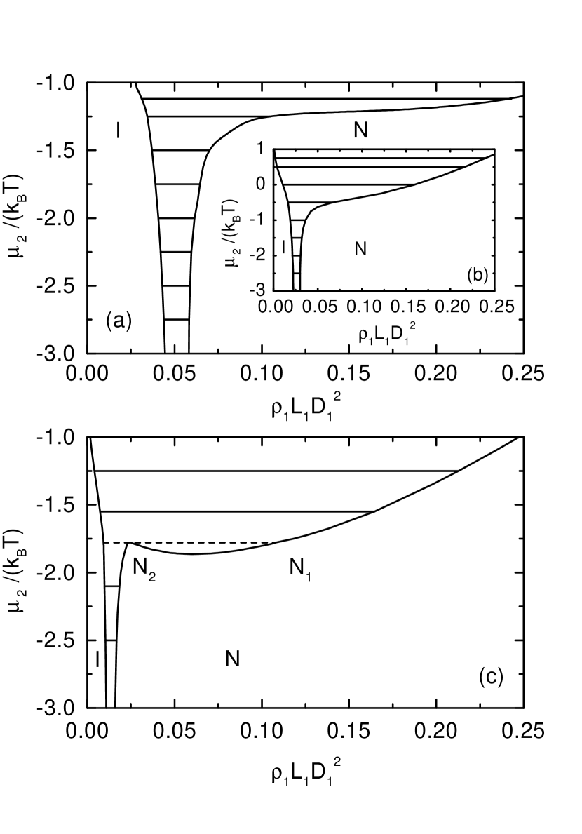
Figure 4: Phase diagram of a fluid consisting of a binary mixture of small platelets [$L_{2}/D_{2}=0.1$] and large platelets [(a): $D_{1}/D_{2}=10$, $L_{1}/D_{1}=0.04$; (b): $D_{1}/D_{2}=5$, $L_{1}/D_{1}=0.04$; (c): $D_{1}/D_{2}=10$, $L_{1}/D_{1}=0.01$] as a function of the chemical potential of the small platelets $\mu_{2}$ and the density of the large platelets $\rho_{1}$. The straight solid lines are tie-lines illustrating isotropic-nematic (I-N) coexistence. The dashed line in (c) marks coexistence of an isotropic phase (I) with two nematic phases (N₁ and N₂) of different compositions.

For large negative chemical potential $\mu_{2}$, the systems exhibit a first oder I-N transition and the density gap at the I-N transition broadens with increasing $\mu_{2}$ in agreement with our previous calculations for binary mixtures of infinitely thin platelets harn:02 . Upon increasing $\mu_{2}$, the phase diagrams presented in Figs. 4, 5 differ qualitatively, and it is worthwhile to distinguish the following cases.

Fig. 4 (a), (b): The width of the I-N transition broadens continuously with increasing $\mu_{2}$. At high densities in the nematic phase, the small platelets are nearly excluded and hence the large platelets are in equilibrium with a reservoir of small platelets. This implies that the pressure of the nematic phase is equal to that of a reservoir of small platelets at a chemical potential $\mu_{2}$.

Fig. 4 (c): Decreasing the aspect ratio $\zeta_{1}=L_{1}/D_{1}$ (as compared to Fig. 4 (a), (b)) at fixed $L_{2}$, $D_{2}$ leads to a smaller width of the I-N transition and a shift of the I-N transition density to smaller values of $\rho_{1}$ as already discussed in the case of monodisperse platelet fluids (see Eq. (58)).

Figure 5: Phase diagram of a fluid consisting of a binary mixture of large thin platelets [$L_{1}/D_{1}=0.01$] and small platelets [(a): $D_{1}/D_{2}=2$, $L_{2}/D_{2}=0.16$; (b): $D_{1}/D_{2}=1.66$, $L_{2}/D_{2}=0.13$; (c): $D_{1}/D_{2}=2$, $L_{2}/D_{2}=0.2$] as a function of the chemical potential of the small platelets $\mu_{2}$ and the density of the large platelets $\rho_{1}$. The straight solid lines are tie-lines illustrating isotropic-nematic (I-N) and nematic-nematic (N₁-N₂) coexistence, respectively. The dashed line in (c) marks coexistence of an isotropic phase (I) with two nematic phases (N₁ and N₂).

The I-N transition ends in an I-N₁-N₂ triple point, at which two nematic phases (N₁, N₂) coexist with an isotropic phase. Above the triple point there is coexistence between a low-density isotropic and a high-density nematic phase. The nematic-nematic (N₁-N₂) coexistence region is bounded by a lower critical point.

Fig. 5 (a), (b): The I-N coexistence regime is bounded by an upper critical point above which a single stable nematic phase is found. The nematic phase demixes into two nematic phases (N₁, N₂) at sufficiently large values of $\mu_{2}$.

Fig. 5 (c): The width of the I-N transition broadens with increasing aspect ratio $\zeta_{2}=L_{2}/D_{2}$ (as compared to Fig. 5 (a), (b)) at fixed $L_{1}$, $D_{1}$. Moreover, the lower critical point of the N₁-N₂ coexistence region shifts to smaller values of $\mu_{2}$, until the N₁-N₂ and I-N coexistence regions start to overlap, giving rise to a triple point.

A simple estimate of the critical aspect ratios required for a depletion-driven demixing transition is obtained from a second virial approximation of the excess free energy functional (16). A straightforward analysis shows that demixing at constant volume is possible, provided the following interaction parameter $\chi(s_{1},s_{2})>0$:

$$\!\!\!\!\!\chi(s_{1},s_{2}) = 2E_{12}(s_{1},s_{2})\!-\!E_{11}(s_{1},s_{1})\!-\!E_{22}(s_{2},s_{2}),\!$$ (62)

with

$$E_{ij}(s_{i},s_{j})=$$ (63)

$$\frac{1}{3}(D_{i}+D_{j})\left[2(D_{i}D_{j}+L_{i}L_{j})(1-s_{i}s_{j})\right.$$

$$+\left.(D_{i}L_{j}+D_{j}L_{i})(1+2s_{i}s_{j})+3(D_{i}L_{i}+D_{j}L_{j})\right],$$

where $i,j=1,2$. The values of the nematic order parameters $s_{1}$ and $s_{2}$ are obtained by a numerical minimization of the grand potential. In order study a possible nematic-nematic demixing transition one may investigate the interaction parameter $\chi(1,1)$:

$$\frac{\chi(1,1)}{D_{1}^{3}}=$$ (64)

$$\left(1+\frac{D_{2}}{D_{1}}\right)^{2}\left(\zeta_{1}+\zeta_{2}\frac{D_{2}}{D_{1}}\right)-8\zeta_{1}-8\zeta_{2}\left(\frac{D_{2}}{D_{1}}\right)^{3}\,,$$

where $\zeta_{1}=L_{1}/D_{1}$ and $\zeta_{2}=L_{2}/D_{2}$. For the model parameters used in Fig. 5, $\chi(1,1)>0$, in agreement with that fact that nematic-nematic demixing has been found by numerical minimization of the FMT grand potential.

Figure 6 displays an alternative representation of the phase diagram shown in Fig. 5 (a) in terms of the number densities of the large and the small platelets $\rho_{1}$ and $\rho_{2}$, respectively.

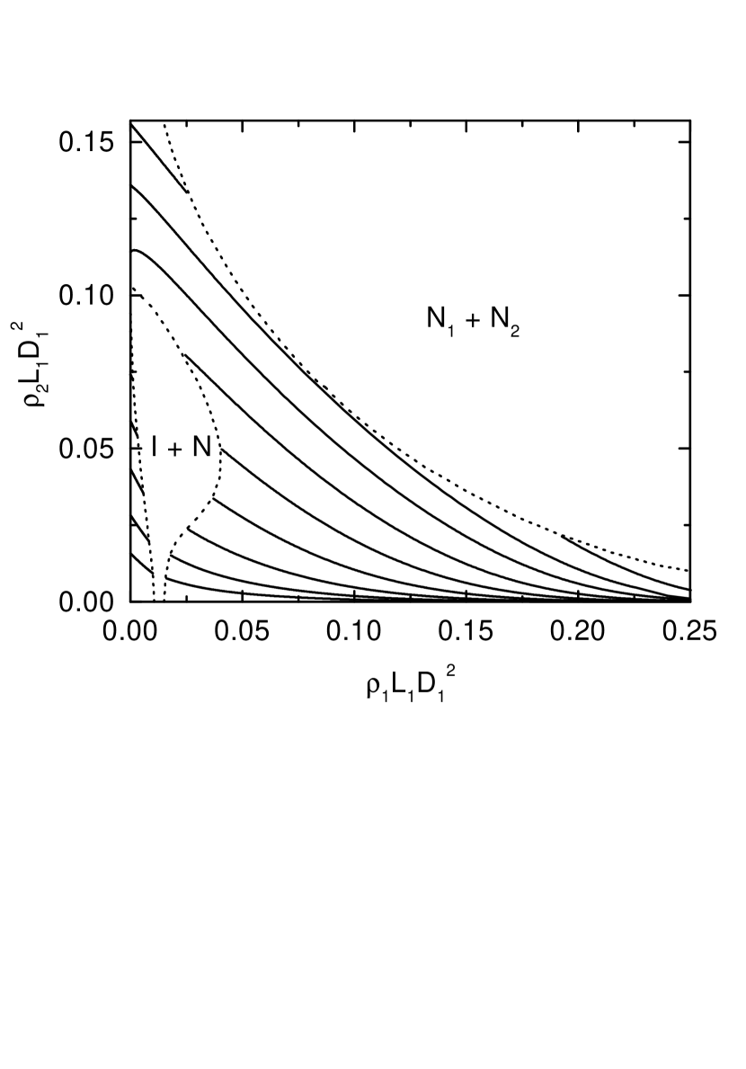
Figure 6: Phase diagram of a binary platelet fluid, corresponding to Fig. 5 (a), in the density-density, i.e., $\rho_{1}$-$\rho_{2}$ plane. The dotted lines indicate phase boundaries. The chemical potential of the small platelets is kept fixed for each solid line and increases from bottom to top: $\mu_{2}/(k_{B}T)=-5,-4,-3,-2,-1,0,1,1.9,3$.

The figure illustrates how the composition of the mixture varies upon increasing the chemical potential (and hence the reservoir density) of the small platelets.

VI Conclusions

We have generalized Zwanzig’s model of cuboids (or parallelepipeds) with only three allowed orientations to the case of monodisperse and bidisperse systems of platelets ($\zeta=L/D<1$). In view of the uncertainties concerning the convergence of the virial series, we have used Rosenfeld’s FMT, along the lines of Cuesta’s work on parallel hard cubes cues:96 to derive a free energy function of the density and the nematic order parameter, which on the basis of earlier experience with other hard core systems, is expected to be quantitatively accurate. In the monodisperse case, the isotropic to nematic transition narrows with increasing aspect ratio $\zeta$. Very rich phase diagrams, involving an isotropic and one or two nematic phases of different concentrations are found for bidisperse systems; the phase diagrams are very sensitive to the size and aspect ratios and although our results can only be considered to be of qualitative significance, due to the restricted number of allowed orientations, we believe that these results clearly point to the possibility of tuning the phase behaviour by appropriate choices of the relative diameters and thicknesses of real platelets. This is of genuine technological importance for the design of clay based drilling fluids mait:00 . Since clay platelets are highly charged, Coulombic interactions must be included in the model and this could lead to major changes in the predicted phase diagrams. Calculations of binary platelet phase diagrams, including Coulombic forces, along the lines of Ref. rowa:02 are under way.

Appendix A Third and fourth virial coefficients for the Zwanzig model of platelets

According to the standard definition of the third virial coefficient involving three particles of species $\beta_{1}$, $\beta_{2}$, $\beta_{3}$ (where here $\beta_{i}=x,y$ or $z$ denote one of of the three possible orientations of the platelets):

$$B_{3}(\beta_{1},\beta_{2},\beta_{3})=$$

$$-\frac{1}{3V}\int d{\bf r}_{1}\,d{\bf r}_{2}\,d{\bf r}_{3}\,f_{\beta_{1},\beta_{2}}({\bf r}_{12})f_{\beta_{1},\beta_{3}}({\bf r}_{13})f_{\beta_{2},\beta_{3}}({\bf r}_{23})$$

$$= -\frac{1}{3}\int d{\bf r}\,d{\bf r}^{\prime}\,f_{\beta_{1},\beta_{2}}({\bf r})f_{\beta_{1},\beta_{3}}({\bf r}^{\prime})f_{\beta_{2},\beta_{3}}({\bf r}-{\bf r}^{\prime})$$

$$= \frac{1}{3}\prod_{\alpha}\int\limits_{-\infty}^{\infty}dr_{\alpha}\,\int\limits_{-\infty}^{\infty}dr^{\prime}_{\alpha}\,\Theta(S_{\alpha;\beta_{1},\beta_{2}}-|r_{\alpha}|)$$ (65)

$$\times\Theta(S_{\alpha;\beta_{1},\beta_{3}}-|r^{\prime}_{\alpha}|)\Theta(S_{\alpha;\beta_{2},\beta_{3}}-|r_{\alpha}-r^{\prime}_{\alpha}|)\,.$$

where $S_{\alpha;\beta_{1},\beta_{2}}=(S_{\alpha;\beta_{1}}+S_{\alpha;\beta_{2}})/2$ and definitions (3) and (4) have been used. The two-dimensional integrals involving Heaviside step functions are easily calculated, and lead to the following results:

$$B_{3}(x,x,x) = 9L^{2}D^{4}\,,$$ (66)

$$B_{3}(x,x,y) = LD^{3}(L+2D)(D+2L)\,,$$ (67)

$$B_{3}(x,y,z) = \frac{1}{3}D^{3}(2L+D)^{3}\,,$$ (68)

while for the isotropic phase (where $\rho_{x}=\rho_{y}=\rho_{z}=\rho/3$), $B_{3}$, as given by (9), reduces to:

$$B_{3} = \frac{2}{27}D^{6}+\frac{16}{9}D^{5}L+\frac{47}{9}D^{4}L^{2}+\frac{52}{27}D^{3}L^{3}\,.$$ (69)

These expressions are easily generalized to the case of binary mixtures of platelets, with the added complication of species indices.

Similarly, there are 4 independent 4-th virial coefficients in the one-component case, corresponding to various orientations of the four particles, namely $B_{4}(x,x,x,x)$, $B_{4}(x,x,x,y)$, $B_{4}(x,x,y,y)$ and $B_{4}(x,x,y,z)$. Each of these has contributions from 4 irreducible diagrams (see Eq. (4.5.13) in hans:86 ) for each set of orientations. The calculations of the multiple integrals are tedious, and we have evaluated $B_{4}$ only for three limiting cases. We find for the isotropic phase:

(a) Long rods, corresponding to the limit $\zeta\to\infty$:

$$B_{4} = -\frac{32}{243}D^{3}L^{6}\,.$$ (70)

(b) Thin platelets, corresponding to the limit $\zeta\to 0$:

$$B_{4} = -\frac{16}{243}D^{9}\,.$$ (71)

(c) Parallel cubes, corresponding to $\zeta=1$:

$$B_{4} = \frac{34}{3}D^{9}\,.$$ (72)

In the case of long rods and thin platelets the fully connected diagram does not contribute to $B_{4}$, and the calculations of the other diagrams is considerably simplified.

References

- (1) See e.g., G. C. Maitland, Current Opinion in Colloid and Interface Science 5, 301, (2000).
- (2) A. Mourchid, A. Delville, J. Lambard, E. Lecolier and P. Levitz, Langmuir 11, 1942 (1995).
- (3) L. Onsager, Ann. (N.Y.) Acad. Sci. 51, 627 (1949).
- (4) R. Eppenga and D. Frenkel, Mol. Phys. 52, 1303 (1984).
- (5) J. A. C. Veerman and D. Frenkel, Phys. Rev. A 45, 5632 (1992).
- (6) F. M. van der Kooij and H. N. W. Lekkerkerker, J. Phys. Chem. B 102, 7829 (1998).
- (7) M. Dijkstra, J.-P. Hansen, and P. A. Madden, Phys. Rev. E 55, 3044 (1997); S. Kutter, J.-P. Hansen, M. Sprik and E. Boek, J. Chem. Phys. 112, 311 (2000).
- (8) F. M. van der Kooij, D. van der Beek, and H. N. W. Lekkerkerker, J. Phys. Chem. B, 105, 1696, (2001).
- (9) H. H. Wensink, G. J. Voerge, and H. N. W. Lekkerkerker, J. Phys. Chem. B, 105, 10610, (2001).
- (10) M. A. Bates and D. Frenkel, J. Chem. Phys., 110, 6553, (1999).
- (11) R. Zwanzig, J. Chem. Phys. 39, 1714 (1963).
- (12) R. Zwanzig, J. Chem. Phys. 24, 855 (1956); W. G. Hoover and A. G. De Rocco, J. Chem. Phys. 36, 3141 (1962); W. G. Hoover and J. C. Poirier, J. Chem. Phys. 38, 327 (1963).
- (13) D. Rowan and J.-P. Hansen, to appear in Phys. Chem. Chem. Phys. (2002).
- (14) F. van Swol and L. V. Woodcock, Mol. Simul. 1, 95, (1987).
- (15) E. Reiss, H. Frisch and J. L. Lebowitz, J. Chem. Phys. 31, 369 (1959).
- (16) Y. Rosenfeld, J. Chem. Phys. 89, 4272 (1988); Y. Rosenfeld, Phys. Rev. Lett. 63, 980 (1989).
- (17) J. A. Cuesta, Phys. Rev. Lett. 76, 3742 (1996); J. A. Cuesta and Y. Martinez-Raton, J. Chem. Phys. 107, 6379 (1997).
- (18) L. Harnau, D. Costa, and J.-P. Hansen, Europhys. Lett. 53, 729 (2001); L. Harnau and S. Dietrich, Phys. Rev. E. 65, 021505 (2002).
- (19) J. P. Straley, J. Chem. Phys. 57, 3694 (1972).
- (20) See e.g., M. Dijkstra, R. van Roij and R. Evans, Phys. Rev. E 59, 5744 (1999), and references therein.
- (21) G. J. Voerge and H. N. W. Lekkerkerker, Rep. Prog. Phys. 55, 1241 (1992); G. J. Voerge and H. N. W. Lekkerkerker, J. Phys. Chem. 97, 3601 (1993); R. van Roij and B. Mulder, J. Phys. Chem. 105, 11237 (1996).
- (22) R. van Roij, B. Mulder and M. Dijkstra, Physica A 261, 374 (1998) and references therein.
- (23) J.-P. Hansen and I. R. McDonald, Theory of Simple Liquids, 2d edition, (Academic Press), London, (1986).
- (24) L. Harnau and S. Dietrich, Phys. Rev. E. submitted.
- (25) J. D. Parsons, Phys. Rev. A 19, 1225 (1979).