Also at ]Institut für Theoretische Physik, Freie Universität Berlin, Arnimallee 14, D-14195 Berlin, Germany.

Anisotropic susceptibilities of thin ferromagnetic films within many-body Green’s function theory

Abstract

Transverse and parallel static susceptibilities of in-plane uniaxial anisotropic ferromagnetic films are calculated using a Heisenberg model within the framework of many-body Green’s function theory. The importance of collective magnetic excitations, in particular in the paramagnetic regime, is demonstrated by comparing with mean field calculations. The paper extends the work of Jensen et al. Jens03 on the monolayer with spin $1/2$ to the multilayer case with arbitrary spin.

1. Introduction

In a recent paper, Jensen et al. Jens03 reported on the measurement of the magnetic susceptibility of a bilayer Co film with an in-plane uniaxial anisotropy. On the basis of a Heisenberg model they determined the isotropic exchange interaction and the magnetic anisotropy within the framework of a Green’s function theory by fitting the interaction parameters of the theory to the measured susceptibilities along the easy and hard axes in the paramagnetic regime, assuming a spin $S=1/2$. In this paper, we generalize the theoretical treatment to the multilayer case and to spins S$>$1/2. We organize the paper as follows. In Section 2 we explain the model and the Green’s function formalism for its solution. Section 3 displays the numerical results. In the final Section 4 we summarize the results and present our conclusions.

2. The model and the Green’s function formalism

We consider a Hamiltonian consisting of a ferromagnetic isotropic Heisenberg exchange interaction with strength ($J_{kl}>0$) between nearest neighbour lattice sites, a uniaxial in-plane exchange anisotropy in the z-direction with strength ($D_{kl}>0$), and an external magnetic field ${\bf B}=(B^{x},0,B^{z})$ confined to the film plane:

$${\cal H}= - \frac{1}{2}\sum_{<kl>}J_{kl}(S_{k}^{-}S_{l}^{+}+S_{k}^{z}S_{l}^{z})-\frac{1}{2}\sum_{<kl>}D_{kl}S_{k}^{z}S_{l}^{z}$$ (1)

$$- \sum_{k}\Big{(}B^{x}\frac{1}{2}(S_{k}^{+}+S_{k}^{-})+B^{z}S_{k}^{z}\Big{)}.$$

Here the notation $S_{k}^{\pm}=S_{k}^{x}\pm iS_{k}^{y}$ is introduced, where $k$ and $l$ are lattice site indices and $<kl>$ indicates summation over nearest neighbours only. In keeping with reference Jens03 , we do not consider the dipole coupling, since it is almost isotropic for the in-plane situation. We note, however, that the formalism is capable of handling this coupling, if so desired, and we refer the reader to references FJKE00 ; FK03 , where we treated the reorientation of the magnetization of ferromagnetic films with anisotropies normal to the film plane. Also in keeping with reference Jens03 , we choose the exchange anisotropy over the single-ion anisotropy, which has the advantage of being simpler to handle in the Green’s function theory. Moreover, we have shown in FK03 that once the strength of the exchange anisotropy is fitted appropriately, the magnetization as a function of the temperature and film thickness behaves very similar to that calculated from the single-ion anisotropy, which may appear somewhat surprising, since the anisotropies originate from very different physical mechanisms. In this paper we shall restrict ourselves to a simple cubic lattice.

In order to generalize the treatment of Jens03 to general spin $S$, we need the following Green’s functions

$$G_{ij,\eta}^{\alpha,mn}(\omega)=\langle\langle S_{i}^{\alpha};(S_{j}^{z})^{m}(S_{j}^{-})^{n}\rangle\rangle_{\omega,\eta}\ ,$$ (2)

where $\alpha=(+,-,z)$ takes care of all directions in space, $\eta=\pm 1$ refers to the anticommutator or commutator Green’s functions, respectively, and $n\geq 1,m\geq 0$ are positive integers, necessary for dealing with higher spin values $S$. For $n=1$ and $m=0$ we will recover the equations of Jens03 .

The exact equations of motion for the Green’s functions are

$$\omega G_{ij,\eta}^{\alpha,mn}(\omega)=A_{ij,\eta}^{\alpha,mn}+\langle\langle[S_{i}^{\alpha},{\cal H}]_{-};(S_{j}^{z})^{m}(S_{j}^{-})^{n}\rangle\rangle_{\omega,\eta}$$ (3)

with the inhomogeneities

$$A_{ij,\eta}^{\alpha,mn}=\langle[S_{i}^{\alpha},(S_{j}^{z})^{m}(S_{j}^{-})^{n}]_{\eta}\rangle,$$ (4)

where $\langle...\rangle=Tr(...e^{-\beta{\cal H}})/Tr(e^{-\beta{\cal H}})$ denotes the thermodynamic expectation value.

After solving these equations, the components of the magnetization can be determined from the Green’s functions via the spectral theorem. A closed system of equations is achieved by decoupling the higher-order Green’s functions on the right hand sides. For the exchange-interaction and exchange-anisotropy terms, we use a generalized Tyablikov- ( RPA-) decoupling

$$\langle\langle S_{i}^{\alpha}S_{k}^{\beta};(S_{j}^{z})^{m}(S_{j}^{-})^{n}\rangle\rangle_{\eta}\simeq\langle S_{i}^{\alpha}\rangle G_{kj,\eta}^{\beta,mn}+\langle S_{k}^{\beta}\rangle G_{ij,\eta}^{\alpha,mn}.$$ (5)

We do not try to do better than RPA because we have shown in earlier workEFJK99 ; HFKTJ02 , by comparing RPA with “exact” Quantum Monte Carlo calculations that the former is quite a good approximation in simple cases.

We now proceed with the formulation of the theory for the multilayer case. After a Fourier transform to momentum space, we obtain, for a film with $N$ layers, $3N$ equations of motion for a $3N$-dimensional Green’s function vector ${\bf G}^{mn}$:

$$(\omega{\bf 1}-{\bf\Gamma}){\bf G}^{mn}_{\eta}={\bf A}^{mn}_{\eta},$$ (6)

where ${\bf 1}$ is the $3N\times 3N$ unit matrix. The Green’s function vectors and inhomogeneity vectors each consist of $N$ three-dimensional subvectors which are characterized by the layer indices $i$ and $j$

$${\bf G}_{ij,\eta}^{mn}({\bf{k},\omega})\ =\left(\begin{array}[]{c}G_{ij,\eta}^{+,mn}({\bf{k}},\omega)\\ G_{ij,\eta}^{-,mn}({\bf{k}},\omega)\\ G_{ij,\eta}^{z,mn}({\bf{k}},\omega)\end{array}\right),\hskip 14.22636pt{\bf A}_{ij,\eta}^{mn}{=}\left(\begin{array}[]{c}A_{ij,\eta}^{+,mn}\\ A_{ij,\eta}^{-,mn}\\ A_{ij,\eta}^{z,mn}\end{array}\right)\;.$$ (7)

The equations of motion are then expressed in terms of these layer vectors and the $3\times 3$ submatrices ${\bf\Gamma}_{ij}$ of the $3N\times 3N$ matrix ${\bf\Gamma}$

$$\left[\omega{\bf 1}-\left(\begin{array}[]{cccc}{\bf\Gamma}_{11}&{\bf\Gamma}_{12}&\ldots&{\bf\Gamma}_{1N}\\ {\bf\Gamma}_{21}&{\bf\Gamma}_{22}&\ldots&{\bf\Gamma}_{2N}\\ \ldots&\ldots&\ldots&\ldots\\ {\bf\Gamma}_{N1}&{\bf\Gamma}_{N2}&\ldots&{\bf\Gamma}_{NN}\end{array}\right)\right]\left[\begin{array}[]{c}{\bf G}_{1j,\eta}\\ {\bf G}_{2j,\eta}\\ \ldots\\ {\bf G}_{Nj,\eta}\end{array}\right]$$ (16)

$$= \left[\begin{array}[]{c}{\bf A}_{1j,\eta}\delta_{1j}\\ {\bf A}_{2j,\eta}\delta_{2j}\\ \ldots\\ {\bf A}_{Nj,\eta}\delta_{Nj}\end{array}\right]\;,\hskip 8.5359ptj=1,...,N\;.$$ (21)

When performing the decouplings according to equation (5), the ${\bf\Gamma}$-matrix reduces to a band matrix with zeros in the ${\bf\Gamma}_{ij}$ sub-matrices, when $j>i+1$ and $j<i-1$. The diagonal sub-matrices ${\bf\Gamma}_{ii}$ are of size $3\times 3$ and have the form

$${\bf\Gamma}_{ii}=\left(\begin{array}[]{@{\hspace*{3mm}}c@{\hspace*{5mm}}c@{\hspace*{5mm}}c@{\hspace*{3mm}}}\hskip 8.53581pt\lx@intercol\hfil\;\;\;H^{z}_{i}\hfil\hskip 14.22636pt&0\hfil\hskip 14.22636pt&-H^{x}_{i}\hfil\hskip 8.53581pt\\ \hskip 8.53581pt\lx@intercol\hfil 0\hfil\hskip 14.22636pt&-H^{z}_{i}\hfil\hskip 14.22636pt&\;\;\;H^{x}_{i}\hfil\hskip 8.53581pt\\ \hskip 8.53581pt\lx@intercol\hfil-\frac{1}{2}\tilde{H}^{x}_{i}\hfil\hskip 14.22636pt&\;\frac{1}{2}\tilde{H}^{x}_{i}\hfil\hskip 14.22636pt&0\hfil\hskip 8.53581pt\end{array}\right)\ .$$ (22)

where

$$H^{z}_{i} = Z_{i}+\langle S_{i}^{z}\rangle J_{ii}(q-\gamma_{\bf k})\ ,$$

$$Z_{i} = B^{z}+D_{ii}q\langle S^{z}_{i}\rangle+(J_{i,i+1}+D_{i,i+1})\langle S_{i+1}^{z}\rangle$$ (23)

$$+(J_{i,i-1}+D_{i,i-1})\langle S_{i-1}^{z}\rangle\ ,$$

$$\tilde{H}^{x}_{i} = B^{x}+\langle S_{i}^{x}\rangle J_{ii}(q-\gamma_{\bf k})+J_{i,i+1}\langle S_{i+1}^{x}\rangle+J_{i,i-1}\langle S_{i-1}^{x}\rangle\ ,$$

$$H^{x}_{i} = \tilde{H}^{x}_{i}-\langle S_{i}^{x}\rangle D_{ii}\gamma_{\bf k}\ .$$

For a square lattice and a lattice constant taken to be unity, $\gamma_{\bf k}=2(\cos k_{x}+\cos k_{z})$, and $q=4$ is the number of intra-layer nearest neighbours. The mean field (MFT) results, which we use later for comparison with Green’s function theory, are obtained by putting $\gamma_{\bf k}=0$; i.e. only the number of nearest neighbour counts, whereas RPA introduces a momentum dependence on the lattice under consideration.

Note that because the momentum dependence in $H_{i}^{x}$ stems from the exchange anisotropy, $\tilde{H}_{i}^{x}\neq H_{i}^{x}$, which prevents a naive extension of the formalism of reference FJKE00 .

The $3\times 3$ off-diagonal sub-matrices ${\bf\Gamma}_{ij}$ for $j=i\pm 1$ are of the form

$${\bf\Gamma}_{ij}=\left(\begin{array}[]{@{\hspace*{3mm}}c@{\hspace*{5mm}}c@{\hspace*{5mm}}c@{\hspace*{3mm}}}\hskip 8.53581pt\lx@intercol\hfil-J_{ij}\langle S_{i}^{z}\rangle\hfil\hskip 14.22636pt&0\hfil\hskip 14.22636pt&\;\;\;(J_{ij}+D_{ij})\langle S_{i}^{x}\rangle\hfil\hskip 8.53581pt\\ \hskip 8.53581pt\lx@intercol\hfil 0\hfil\hskip 14.22636pt&\;\;J_{ij}\langle S_{i}^{z}\rangle\hfil\hskip 14.22636pt&-(J_{ij}+D_{ij)}\langle S_{i}^{x}\rangle\hfil\hskip 8.53581pt\\ \hskip 8.53581pt\lx@intercol\hfil\frac{1}{2}J_{ij}\langle S_{i}^{x}\rangle\hfil\hskip 14.22636pt&-\frac{1}{2}J_{ij}\langle S_{i}^{x}\rangle\hfil\hskip 14.22636pt&0\hfil\hskip 8.53581pt\end{array}\right)\;.$$ (24)

The treatment of multilayers is only practicable when using the eigenvector method developed in reference FJKE00 . The essential features are as follows. One starts with a transformation, which diagonalizes the ${\bf\Gamma}$-matrix of equation (6)

$${\bf L\Gamma R}={\bf\Omega},$$ (25)

where ${\bf\Omega}$ is a diagonal matrix with eigenvalues $\omega_{\tau}$ ($\tau=1,...,3N$), and the transformation matrix R and its inverse ${\bf R}^{-1}={\bf L}$ are obtained from the right eigenvectors of ${\bf\Gamma}$ as columns and from the left eigenvectors as rows, respectively. These matrices are normalized to unity: RL=LR=1.

Multiplying the equation of motion (6) from the left by L and inserting 1=RL one finds

$$(\omega{\bf 1}-{\bf\Omega}){\bf L}{\bf G}_{\eta}^{mn}={\bf LA}_{\eta}^{mn}.$$ (26)

Defining ${\cal G}_{\eta}^{mn}={\bf LG}_{\eta}^{mn}$ and ${\cal A}_{\eta}^{mn}={\bf LA}_{\eta}^{mn}$ one obtains

$$(\omega{\bf 1}-{\bf\Omega}){\cal G}_{\eta}^{mn}={\cal A}_{\eta}^{mn}.$$ (27)

${\cal G}_{\eta}^{mn}$ is a vector of new Green’s functions, each component $\tau$ of which has but a single pole

$${\cal G}_{\eta}^{mn,\tau}=\frac{{\cal A}_{\eta}^{mn,\tau}}{\omega-\omega_{\tau}}\ .$$ (28)

This is the important point because it allows application of the spectral theorem, e.g. GHE01 , to each component separately. We obtain for the component $\tau$ of correlation vector ${\cal C}^{mn}={\bf L}{\bf C}^{mn}$ ( where ${\bf C}^{mn}=\langle(S^{z})^{m}(S^{-})^{n}S^{\alpha}\rangle$ with $(\alpha=+,-,z)$)

$${\cal C}^{mn,\tau}=\frac{{\cal A}_{\eta}^{mn,\tau}}{e^{\beta\omega_{\tau}}+\eta}+\frac{1}{2}(1-\eta)\frac{1}{2}\lim_{\omega\rightarrow 0}\omega\frac{{\cal A}_{\eta=+1}^{mn,\tau}}{\omega-\omega_{\tau}}.$$ (29)

We emphasize that when ($\eta=-1$), the second term of this equation, which is due to the anticommutator Green’s function, has to be taken into account. This term occurs for $\omega_{\tau}=0$ and can be simplified by using the relation between anticommutator and commutator

$${\cal A}_{\eta=+1}^{mn,0}={\cal A}^{mn,0}_{\eta=-1}+2{\cal C}^{mn,0}={\bf L}_{0}(A_{\eta=-1}^{mn}+2{\bf C}^{mn}),$$ (30)

where the index $\tau=0$ refers to the eigenvector with $\omega_{\tau}=0$.

The term ${\bf L}_{0}A_{\eta=-1}^{mn}=0$ vanishes due to the fact that the commutator Green’s function has to be regular at the origin

$$\lim_{\omega\rightarrow 0}\omega G_{\eta=-1}^{\alpha,mn}=0,$$ (31)

which leads to the regularity conditions:

$$\tilde{H}^{x}A_{\eta=-1}^{+,mn}+\tilde{H}^{x}A_{\eta=-1}^{-,mn}+2H^{z}A_{\eta=-1}^{z,mn}=0.$$ (32)

For details, see reference FJKE00 .

This is equivalent to

$${\bf L}_{0}A_{\eta=-1}^{mn}=0,$$ (33)

because the left eigenvector of the ${\bf\Gamma}$-matrix with eigenvector zero has the structure (see also equation (40) below)

$${\bf L}_{0}\propto(\tilde{H}^{x},\tilde{H}^{x},2H^{z}).$$ (34)

For more details concerning the use of the regularity conditions, see refs. FJKE00 ; FK03 .

The equations for the correlations are then obtained by multiplying equation (29) from the left with ${\bf R}$ and using equation (33); i.e.

$${\bf C}={\bf R}{\bf{\cal E}}{\bf L}{\bf A}+{\bf R}_{0}{\bf L}_{0}{\bf C},$$ (35)

where ${\bf{\cal E}}$ is a diagonal matrix with matrix elements ${\cal E}_{ij}=\delta_{ij}(e^{\beta\omega_{i}}-1)^{-1}$ for eigenvalues $\omega_{i}\neq 0$, and $0$ for eigenvalues $\omega_{i}=0$.

A problem associated with this equation is that the exchange anisotropy introduces a momentum dependence into the projection operator ${\bf R}_{0}{\bf L}_{0}$. Consequently, when the Fourier transform to real space is performed, the projector cannot be taken out of the integral as is possible in the case of the Anderson Callen decoupling of the single-ion anisotropy FJKE00 , where the projector turns out to be momentum independent. The solution is to eliminate one component of the projector by a transformation of equation (35), which is sufficient to establish the integral equations of the eigenvector method.

The adequate transformation is found to be

$${\bf T}^{-1}=\frac{1}{2}\left(\begin{array}[]{ccc}1&1&0\\ -1&1&0\\ 0&0&2\end{array}\right)\ \ \ \ \ \ \ {\bf T}=\left(\begin{array}[]{ccc}1&-1&0\\ 1&1&0\\ 0&0&1\end{array}\right)$$ (36)

with ${\bf T}^{-1}{\bf T}={\bf 1}$.

Applying this transformation to equation (35) considered as a monolayer problem

$${\bf T}^{-1}{\bf C}={\bf T}^{-1}{\bf R{\cal E}LTT}^{-1}{\bf A}+{\bf T}^{-1}{\bf R}_{0}{\bf L}_{0}{\bf TT}^{-1}{\bf C}$$ (37)

transforms the second component of the vector ${\bf T}^{-1}{\bf R}_{0}{\bf L}_{0}{\bf TT}^{-1}{\bf C}$ to zero. This can be seen when inserting the explicit expressions for the eigenvalues and eigenvectors for the monolayer. The eigenvalues of the ${\bf\Gamma}$-matrix in this case are

$$\omega_{1}=0;\ \ \omega_{2,3}=\pm\varepsilon_{\bf k}=\pm\sqrt{H^{z}H^{z}+\tilde{H^{x}}H^{x}},$$ (38)

the right eigenvectors are the columns of the matrix

$${\bf R}=\left(\begin{array}[]{ccc}\frac{H^{x}}{H^{z}}&\frac{-(\epsilon_{\bf k}+H^{z})}{\tilde{H}^{x}}&\frac{(\epsilon_{\bf k}-H^{z})}{\tilde{H}^{x}}\\ \frac{H^{x}}{H^{z}}&\frac{(\epsilon_{\bf k}-H^{z})}{\tilde{H}^{x}}&\frac{-(\epsilon_{\bf k}+H^{z})}{\tilde{H}^{x}}\\ 1&1&1\end{array}\right)\ ,$$ (39)

and the left eigenvectors are the rows of the matrix

$${\bf L}=\frac{1}{4\epsilon_{\bf k}^{2}}\left(\begin{array}[]{ccc}2\tilde{H^{x}}H^{z}&2\tilde{H^{x}}H^{z}&4H^{z}H^{z}\\ -(\epsilon_{\bf k}+H^{z})\tilde{H}^{x}&(\epsilon_{\bf k}-H^{z})\tilde{H}^{x}&2H^{x}\tilde{H}^{x}\\ (\epsilon_{\bf k}-H^{z})\tilde{H}^{x}&-(\epsilon_{\bf k}+H^{z})\tilde{H}^{x}&2H^{x}\tilde{H}^{x}\end{array}\right)\ .$$ (40)

The second row of the transformed equation (37), together with the regularity conditions (32), leads to one integral equation for the correlations for each ($m,n$)-pair.

The eigenvector method can immediately be generalized to the case of $N$ layers by transforming equation (35) (extended to $3N$-dimensions) with a $3N\times 3N$-matrix ${\bf T^{-1}}$ having the $3\times 3$ $T^{-1}$ sub-matrices (36) on the diagonal.

Before showing numerical results for $S>1/2$ and for multilayers we derive the equations for the monolayer and $S=1/2$ of reference Jens03 from equation (37).

Using equations (39,40), one obtains from the second row of equation (37) for the monolayer and for general spin

$$C^{+,mn}-C^{-,mn}+\frac{1}{2}(A^{+,mn}_{\eta=-1}-A^{-,mn}_{\eta=-1})=$$

$$\frac{1}{2}(A^{+,mn}_{\eta=-1}+A^{-,mn}_{\eta=-1})\frac{1}{N}\sum_{\bf k}\frac{\varepsilon_{\bf k}}{H^{z}}\coth({\beta\varepsilon_{\bf k}/2})$$ (41)

and from the first row

$$C^{+,mn}-C^{-,mn}+\frac{1}{2}(A^{+,mn}_{\eta=-1}+A^{-,mn}_{\eta=-1})=$$ (42)

$$\frac{2H^{x}}{H^{z}}C^{z,mn}+A^{z,mn}_{\eta=-1}\frac{H^{x}}{H^{z}}$$

$$+\frac{1}{2}(A^{+,mn}_{\eta=-1}-A^{-,mn}_{\eta=-1})\frac{1}{N}\sum_{\bf k}\frac{\varepsilon_{\bf k}}{H^{z}}\coth({\beta\varepsilon_{\bf k}/2}).$$

The equations for $S=1/2$ are obtained from these equations for $n=1,m=0$, i.e. $C^{-,01}=\langle S^{-}S^{-}\rangle=0$, $C^{+,01}=\langle S^{-}S^{+}\rangle=1/2-\langle S^{z}\rangle$, $A^{-,01}_{\eta=-1}=0$, $A^{+,01}_{\eta=-1}=2\langle S^{z}\rangle$, $C^{z,01}=\langle S^{-}S^{z}\rangle=1/2\langle S^{x}\rangle$, and from the regularity condition (32) $\langle S^{z}\rangle=(H^{z}/\tilde{H^{x}})\langle S^{x}\rangle$:

$$\frac{1}{2}=\langle S^{z}\rangle\frac{1}{N}\sum_{\bf k}\frac{\varepsilon_{\bf k}}{H^{z}}\coth({\beta\varepsilon_{\bf k}/2}),$$ (43)

and

$$\frac{1}{2}=\langle S^{x}\rangle\frac{1}{N}\sum_{\bf k}\frac{\varepsilon_{\bf k}}{\tilde{H^{x}}}\coth({\beta\varepsilon_{\bf k}/2}),$$ (44)

which are the equations used in ref.Jens03 .

For $S>1/2$ and for the multilayer case, the eigenvectors have to be calculated numerically and the system of integral equations obtained from the Fourier transform of equations (37) to real space has to be solved self-consistently, which is done by the curve-following method described in detail in FKS02 .

3. Numerical results

3.1. The monolayer with arbitrary spin ${\bf S}$

We start by showing results for the magnetizations $\langle S^{z}\rangle$ and $\langle S^{x}\rangle$ with respect to the easy and hard axes of a monolayer with various spin values $S$. It turns out that one obtains fairly universal curves when scaling the parameters of the model as $\tilde{J}/S(S+1)=J,\tilde{D}/S(S+1)=D$, and $\tilde{B}^{x(z)}/S=B^{x(z)}$. In the present paper we restrict ourselves to the case where the exchange interaction and exchange anisotropy parameters are the same for all layers and interlayer couplings. The program is, however, written in such a way that different parameters can be easily introduced.

Using the scaled variables, the Curie temperatures $T_{C}(S)$ collapse to a single universal value (the same for each spin $S$) both in mean field theory (MFT) and in the random phase approximation (RPA).

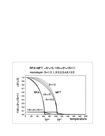
Figure 1: The ‘universal’ magnetizations $\langle S^{z}\rangle/S$ and $100*\langle S^{x}\rangle/(S+1)$ of an anisotropic ferromagnetic Heisenberg monolayer for a square lattice are shown as functions of the temperature for $S=1/2,1,3/2,2,3,4,6,13/2$. Comparison is made between Green’s function (RPA) and mean field (MFT) calculations using the exchange interaction $\tilde{J}=75$, the exchange anisotropy $\tilde{D}=3.75$ (corresponding to $J=100,D=5$ of the S=1/2 case of Ref.Jens03 ) and small magnetic fields $\tilde{B}^{x}=\tilde{B}^{z}=0.01$.

This is shown in Fig.1, where MFT and RPA results for $\langle S^{z}\rangle/S$ and $100\times\langle S^{x}\rangle/(S+1)$ are displayed as functions of the temperature for the spin values $S=1/2,1,3/2,2,3,4,6,13/2$. For the exchange interaction and exchange anisotropy, we use the same parameters as in Ref. Jens03 , which is the S=1/2 monolayer case in our investigations. The calculations for Fig.1 are done with small fields ($\tilde{B}^{x}=\tilde{B}^{z}=0.01$); this stabilizes the numerical algorithm. Whereas $\langle S^{z}\rangle/S$ in RPA is universal over the whole temperature range, the corresponding MFT curves as function of the temperature split somewhat, reaching a saturation for large spin values S (approaching the classical limit). The curves $100\times\langle S^{x}\rangle/(S+1)$ have the same universal value in MFT and RPA for $T<T_{C}^{RPA(MFT)}$ (Because of the very small $B^{x}$ field we introduced the factor 100 to make the curves visible). The reason why the values for $\langle S^{x}\rangle/(S+1)$ coincide below the Curie temperature is that the magnetization in $x$-direction depends only on the number of nearest neighbours. This can be understood from equation (32) from which one obtains with ($n=1,m=0$)

$$\langle S^{x}\rangle=\lim_{B^{z}\rightarrow 0}\frac{\tilde{H^{x}}}{H^{z}}=\frac{B^{x}}{Dq}=\frac{\tilde{B}^{x}S(S+1)}{\tilde{D}qS}.$$ (45)

This explains the universality of $\langle S^{x}\rangle/(S+1)=\tilde{B}^{x}/(\tilde{D}q)$, where $q=4$ is the number of nearest neighbours for the square monolayer. The fact that the universal Curie temperature $T_{C}^{RPA}(S)$ is only about one half of $T_{C}^{MFT}(S)$ for the monolayer is due to the action of collective excitations (magnons=spin waves), which are completely absent in MFT.

Spin waves also have significant effects on the susceptibilities (in particular in the paramagnetic regime $T>T_{C}$) with respect to the easy ($\chi_{zz}$) and hard ($\chi_{xx}$) axes. The susceptibilities are calculated as differential quotients

$$\chi_{zz} = \Big{(}\langle S^{z}(B^{z})\rangle-\langle S^{z}(0)\rangle\Big{)}/B^{z}$$

$$\chi_{xx} = \Big{(}\langle S^{x}(B^{x})\rangle-\langle S^{x}(0)\rangle\Big{)}/B^{x},$$ (46)

where the use of $B^{z}=B^{x}=0.01/S$ turns out to be small enough to get good numerical estimates of the quotients; smaller fields would only be necessary to get better estimates close to the divergence of $\chi_{zz}$ at $T_{C}$; however, the errors in the inverse susceptibilities $\chi_{zz}^{-1}$ and $\chi_{xx}^{-1}$ at this point are not noticeable in the figures. The inverse susceptibilities as functions of the temperature can be brought into near coinicidence with a single universal curve if they are multiplied with a factor $S(S+1)$, especially in the paramagnetic regime.

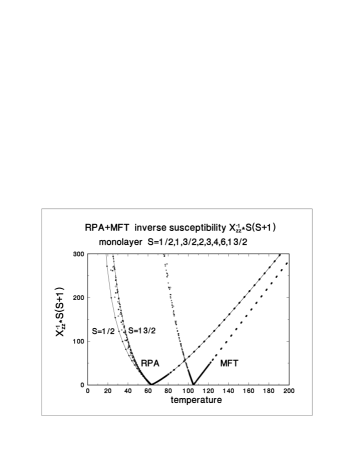
Figure 2: ‘Universal’ inverse susceptibilities $\chi_{zz}^{-1}*S(S+1)$ along the easy axis of an anisotropic ferromagnetic Heisenberg monolayer for a square lattice as functions of the temperature for $S=1/2,1,3/2,2,3.4,6,13/2$. Comparison is made between Green’s function (RPA) and mean field (MFT) calculations.

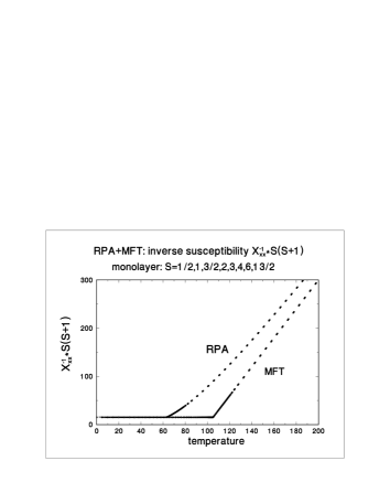
Figure 3: The ‘universal’ inverse susceptibilities $\chi_{xx}^{-1}*S(S+1)$ along the hard axis of an anisotropic ferromagnetic Heisenberg monolayer for a square lattice are shown as functions of the temperature for $S=1/2,1,3/2,2,3,4,6,13/2$. Comparison is made between the results of Green’s function (RPA) and mean field (MFT) calculations.

In Fig.2 we compare RPA and MFT calculations for the inverse susceptibility $\chi_{zz}^{-1}S(S+1)$ along the easy axis. As in Fig. 1, there is a shift in the Curie temperatures in going from RPA to MFT. For $T<T_{C}$, the MFT result behaves more universally than that of RPA; above the Curie temperature, both results are nearly universal. $\chi_{zz}^{-1(MFT)}*S(S+1)$ is a straight line $\propto(T-T_{C}^{MFT})$ like a Curie-Weiss law. For $S=1/2$, one finds analytically from equation (43) in the limit $\langle S^{z}\rangle\rightarrow 0,T\rightarrow{\rm large}$, that

$$S(S+1)\chi_{zz}^{-1(MFT)}=\frac{3}{4}4(T-T_{C}^{MFT}),$$ (47)

where $T_{C}^{MFT}=J+D$. The inverse RPA susceptibility $\chi_{zz}^{-1(RPA)}*S(S+1)$ is curved for $T>T_{C}^{RPA}$ due to magnon effects. This is a behaviour known from isotropic bulk ferromagnets, but the effect is significantly stronger for a monolayer.

An analogous universality is obtained for the inverse suceptibility $\chi_{xx}^{-1}*S(S+1)$. The results are shown in Fig.3. Contrary to the curve for $\chi_{zz}^{-1}$, the hard axis susceptibility does not go to zero at $T=T_{C}$. For $T<T_{C}$ one has the same universal constant in RPA and MFT, which can be calculated analytically for the monolayer $\chi_{xx}^{-1}*S(S+1)=\tilde{D}q$ from equation (45). The slopes of the curves for $T>T_{C}$ are, however, different. The MFT again yields a straight line, whereas the RPA result is curved and approaches a straight line only for very large T. Hence, we see that owing to the scaling properties, it is not necessary to do calculations for each spin value separately. It suffices to do calculations for one spin value and then to apply scaling to obtain the results for other spin values.

3.2. Multilayers at fixed spin S

Next we discuss the multilayer case for fixed spin. We use the example of spin $S=1/2$ (We have also considered multilayers with spins $S>1/2$. The results scale with respect to the spin as in the monolayer case).

Curie temperatures as function of the layer thickness are shown in Fig.4. The difference between RPA and MFT is largest for the monolayer, where $T^{RPA}_{C}\simeq 0.60\ T^{MFT}_{C}$ and shrinks to $T^{RPA}_{C}\simeq 0.80\ T^{MFT}_{C}$ for a film with N=19 layers, where one is approaching the bulk value.

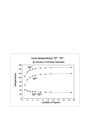
Figure 4: Curie temperatures of ferromagnetic films with spin $S=1/2$ are shown as functions of the film thickness for MFT ($T_{C}^{MFT}$) and RPA ($T_{C}^{RPA}$). The difference $T_{C}^{MFT}-T_{C}^{RPA}$ shrinks by a about a factor of two when going from the monolayer to the bulk limit.

To further emphasize the difference between RPA and MFT, we show in Figs. 5 and 6 the inverse susceptibilities $\chi_{zz}^{-1}$ and $\chi_{xx}^{-1}$ as functions of the temperature. To avoid cluttering the figures, we plot only the results of the monolayer (N=1) and the film with the maximum number of layers (N=19), which is close to the bulk limit because the Curie temperatures saturate with increasing number of layers N. In each case, we observe the shift in the Curie temperatures between RPA and MFT corresponding to Fig.4.

Figure 5: The inverse susceptibilities $\chi_{zz}^{-1}*S(S+1)$ along the easy axisof a ferromagnetic film with spin $S=1/2$ for RPA and MFT are shown as a function of the temperature for a monolayer (N=1) and a multilayer (N=19).

Figure 6: The inverse susceptibilities $\chi_{xx}^{-1}*S(S+1)$ along the hard axis of a ferromagnetic film with spin $S=1/2$ for RPA and MFT are shown as a function of the temperature for a monolayer (N=1) and a multilayer (N=19).

Above the Curie temperature, the inverse susceptibilities are straight lines in the mean field case and curved lines in RPA. The slopes of the curves, however, are different for each film thickness. This is seen most clearly if one normalizes the temperature scale to the Curie temperatures $T_{C}(N)$. The slopes in MFT increase with increasing film thickness, and in RPA the curvature decreases with increasing number of layers, as shown in fig.7.

For $T\leq T_{C}$ the inverse susceptibility $\chi_{xx}^{-1}$ is constant, having the same value in MFT and RPA but depending on the number of layers. The reason for the layer-dependence is that, with increasing film thickness, the number of nearest neighbours increases and therefore one has an increase in the inverse susceptibility. For the square lattice monolayer and bilayer, the values can be calculated analytically from the regularity condition (32): $\chi_{xx}^{-1}(N=1)=\tilde{D}q$ and $\chi_{xx}^{-1}(N=2)=\tilde{D}(q+1)$, with $q=4$ for a square lattice. From the value of $\chi_{xx}^{-1}$ at $T=T_{C}$, one can obtain an estimate of the exchange anisotropy strength parameter D, which, together with the Curie temperature, which depends on the exchange interaction strength J and on the exchange anisotropy strength D, affords an estimation of J. As the number of layers $N$ increases, the relative weights of the layers having two neighbouring layers increases, since it is only the sites in the surface layers which are restricted to having one nearest neighbour in the next layer; hence $\chi_{xx}^{-1}$ slowly increases (see Fig. 8).

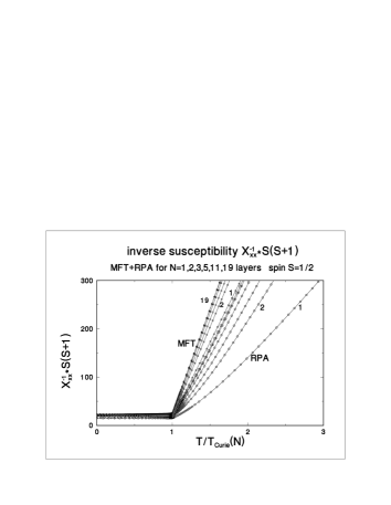
Figure 7: The inverse susceptibilities $\chi_{xx}^{-1}*S(S+1)$ along the hard axis of a ferromagnetic film with spin $S=1/2$ for RPA and MFT are shown as a function of the reduced temperature $T/T_{Curie}(N)$ for N=1,2,3,5,11,19 layers.

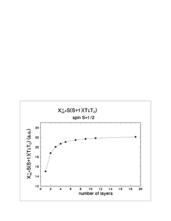
Figure 8: The inverse susceptibilities $\chi_{xx}^{-1}*S(S+1)$ along the hard axis at the Curie temperatures of a ferromagnetic film with spin $S=1/2$ for RPA are shown as a function of the film thickness.

4. Summary and conclusion

We have generalized the many-body Green’s function treatment for calculating in-plane anisotropic static susceptibilities of ferromagnetic films to arbitrary spin $S$ and to multilayers. In particular, we have emphasized the difference in the results from a Green’s function theory (RPA) and mean field theory (MFT), pointing out the importance of spin waves, which are absent in MFT. All results discussed below refer to a simple cubic lattice.

By introducing scaled variables, we were able to show that the magnetic properties of thin ferromagnetic films with in-plane anisotropy manifest nearly universal behaviour. Plotting $\langle S^{z}\rangle/S$ and $\langle S^{x}\rangle/(S+1)$ as functions of the temperature reveals a nearly universal behaviour over the whole temperature range for RPA, whereas $\langle S^{z}\rangle/S$ for MFT shows a small dependence on S. The main difference between RPA and MFT is in the universal Curie temperature which, for the monolayer, is nearly a factor of two larger in MFT than in RPA, $T_{C}^{MFT}\simeq 2*T_{C}^{RPA}$, due to spin wave effects. The hard-axis magnetization $\langle S^{x}\rangle$ has the same constant value in RPA and MFT for $T\leq T_{C}$ because it depends only on the number of nearest neighbours and not on the momentum of the lattice. The inverse susceptibilities along the easy and hard axes also behave universally when scaled as $\chi_{zz}^{-1}*S(S+1)$ and $\chi_{xx}^{-1}*S(S+1)$, particularly in the paramagnetic regime. The difference between MFT and RPA consists in the shift of the Curie temperatures and the behaviour in the paramagnetic region ($T>T_{C}$). Whereas the MFT inverse susceptibilities are linear in $(T-T_{C}^{MFT})$ (a Curie-Weiss-like behaviour), the RPA susceptibilities are curved, owing to spin-wave effects, and approach a straight line only asymptotically for very large temperatures. As long as one scales with respect to the spin $S$ there is no qualitative change in the physical picture from that discussed in Ref. Jens03 for spin $S=1/2$. It is not necessary to perform calculations for each spin value separately. Instead, it is sufficient to calculate the results for one spin value and to apply scaling. This is one of the main results of the paper.

For the multilayers at a fixed spin $S$, the Curie temperature increases with increasing film thickness, approaching the bulk limit around a film consisting of $N\simeq 19$ layers. The difference between the Curie temperatures for MFT and RPA decreases with increasing film thickness from $T_{C}^{MFT}/T_{C}^{RPA}(N=1)\simeq 2$ to $T_{C}^{MFT}/T_{C}^{RPA}(N=1)\simeq 1.3$, which shows that the spin wave effects are strongest for the monolayer. In MFT, the inverse susceptibilities show a linear Curie-Weiss behaviour for $T>T_{C}$, whereas the RPA results are curved. When plotting the inverse susceptibilities as a function of the normalized temperatures $T/T_{C}(N)$ the slopes of the straight lines of MFT increase with increasing layer number, whereas the curvatures of RPA decrease with increasing film thickness. From the curvatures of the inverse susceptibilities it is thus possible to deduce the number of layers, which might be a way to extract information on the film thickness from experiment. For $T\leq T_{C}$, the inverse hard axis susceptibilites $\chi_{xx}^{-1}$ are constants, but their value increases with increasing layer thickness, although not very strongly, which allows one to discriminate between films with differing numbers of layers. From $\chi_{xx}^{-1}(T\leq T_{C})$, one can get in principle information about the exchange anisotropy strength, whereas the value of the Curie temperature depends on both the exchange interaction and the exchange anisotropy strengths. All the results discussed might be modified by a layer-dependence of the exchange interaction and exchange anisotropy or, when a different lattice type has to be considered. Other effects like domain wall motion or vortex excitations, which are not treated in the theory above, could also lead to modifications.

The calculations here demonstrate that we are technically able to calculate the magnetic properties of in-plane anisotropic ferromagnetic multilayer films with $S\geq 1/2$. Hopefully, some of the predictions of the present calculations can be verified experimentally in the future, in particular with respect to the hard axis susceptibility. This might be possible if the experimental techniques discussed in Ref. Jens03 , where experimental results on a bilayer are reported, can be improved. High precision measurements of anisotropic susceptibilities of thin films, particularly above $T_{C}$, are called for, which is certainly a challenge for experimentalists.

We are indebted to P.J. Jensen for useful discussions.

References

• (1) P.J. Jensen, S. Knappmann, W. Wulfhekel, H.P. Oepen, cond-mat/0303320 (2003), accepted for publication in Phys. Rev. B.
• (2) P. Fröbrich, P.J. Jensen, P.J. Kuntz, A. Ecker, Eur. Phys. J. B 18, 579 (2000).
• (3) P. Fröbrich, P.J. Kuntz, M. Saber, Ann. Phys. (Leipzig) 11, 387 (2002).
• (4) P. Fröbrich, P.J. Kuntz, Eur. Phys. J. B 32, 445 (2003).
• (5) A. Ecker, P. Fröbrich, P.J. Jensen, P.J. Kuntz, J. Phys.: Condens. Matter 11, 1557 (1999).
• (6) P. Henelius, P. Fröbrich, P.J. Kuntz, C. Timm, P.J. Jensen, Phys. Rev. B 66, 094407 (2002).
• (7) W. Gasser, E. Heiner, and K. Elk, in ‘Greensche Funktionen in der Festkörper- und Vielteilchenphysik’, Wiley-VHC, Berlin, 2001, Chapter 3.3.