Exact asymptotic form of the exchange interactions between shallow centers in doped semiconductors

Abstract

The method developed in [L. P. Gor’kov and L. P. Pitaevskii, Sov. Phys. Dokl. 8, 788 (1964); C. Herring and M. Flicker, Phys. Rev. 134, A362 (1964)] to calculate the asymptotic form of exchange interactions between hydrogen atoms in the ground state is extended to excited states. The approach is then applied to shallow centers in semiconductors. The problem of the asymptotic dependence of the exchange interactions in semiconductors is complicated by the multiple degeneracy of the ground state of an impurity (donor or acceptor) center in valley or band indices, crystalline anisotropy and strong spin-orbital interactions, especially for acceptor centers in III-V and II-VI groups semiconductors. Properties of two coupled centers in the dilute limit can be accessed experimentally, and the knowledge of the exact asymptotic expressions, in addition to being of fundamental interest, must be very helpful for numerical calculations and for interpolation of exchange forces in the case of intermediate concentrations. Our main conclusion concerns the sign of the magnetic interaction — the ground state of a pair is always non-magnetic. Behavior of the exchange interactions in applied magnetic fields is also discussed.

PACS number(s): 71.70.Gm, 71.55.Eq

I Introduction

Ferromagnetism in diluted III-V semiconductors has recently attracted considerable attention for technologically appealing possibility of integration of spin degrees of freedom into semiconductor devices. In the most intensively studied compound of this group Ga_1-xMn_xAs the ferromagnetic transition temperatures in thin annealed epitaxially grown layers as high as $T_{C}>150$K for $x\sim 8$% have been reported ku03 .

The transition metal impurities in these materials substitute for the atoms of the III group and act as both localized spins ($S=5/2$ for Mn due to half-filled $d$-shell) and as acceptors doping the system with one hole. However, the system is highly compensated presumably owing to double donor antisites (V group elements substituted for III group elements) and metastable interstitial transition metal impurities.

A major not fully resolved issue is the mechanism governing ferromagnetism in these compounds. Despite high disorder in these non-equilibrium epitaxially grown films, RKKY interaction seems to be the most plausible cause of Mn spin-spin interaction dietl01 .

Meanwhile, we want to indicate that magnetic interactions in semiconductors are not well understood yet even in a much simpler case of electrons localized on non-magnetic impurities. Whereas two hydrogen atoms at large distances are known to interact antiferromagnetically, the sign of the interaction between donors/acceptors is not obvious because of the band degeneracies as well as strong spin-orbital interaction present.

To the best of our knowledge, exchange interaction between donors was considered only in Ref. andres81 in the Heitler-London approximation which is known to be incorrect at large separationsherring62 ; gorkov64 ; herring64 . Besides, in Ref. andres81 an isotropic hydrogen-like model was adopted in contrast to real semiconductors that have strong anisotropy of conduction band valleys. In Section III below we compare our results for donors to those of Ref. andres81 .

The purpose of the present paper is to obtain asymptotically exact formulas for the exchange interaction between two shallow centers at large separations. Although our results are pertinent to low impurity concentrations, this information would be necessary for interpolating results of numerical calculations to shorter inter-impurity separations — higher impurity concentrations.

The Heitler-London scheme, which considers exchange with the alien atom as perturbation, is inapplicable herring62 to electron exchange at large separations $R$, because the tunneling takes place through a region where interactions with both atomic residues and between the electrons themselves are comparable. As a matter of fact, the Heitler-London expression for the exchange between two hydrogen atoms incorrectly changes sign at large inter-atom separations. The correct approach to the asymptotic exchange, that accurately accounted for the interaction between the electrons and ionic residues during the exchange process, was proposed in gorkov64 ; herring64 . The magnitude of the exchange was expressed as an integral of the probability current over the 5-dimensional median hyperplane separating two regions of electron localization in their 6-dimensional coordinate space.

Before proceeding to the corresponding problem in semiconductors we list a number of extensions of the method gorkov64 ; herring64 to other problems in atomic physics. In smirnov65 a generalization was made for two atoms with non-equal binding energies of electrons in $s$-states. It turned out, however, that in order for the method to be applicable, the two energies should be close, which severely restricted the applicable range of $R$ (see the discussion in chibisov88 ). In Ref. umanskii68 exchange integrals between degenerate $s$- and $p$- states have been calculated starting from Wigner-Witmer classification of the molecular states (see also nikitin84 ). Exchange integrals between higher orbital momentum $l$ states were calculated in hadinger93 . In papers ponomarev99 the method gorkov64 ; herring64 was applied to get interpolated formulas down to small $R$ and to study two-dimensional electrons localized on out-of-plane impurities. But to the best of our knowledge, multiple degeneracy of donor or acceptor levels in real semiconductors has never been addressed.

In this paper we extend the median-plane method to asymptotic exchange between shallow impurities in semiconductors with localized carriers in degenerate and non-spherically symmetric bands. We also study how spin-orbital interaction and external magnetic field influence the exchange.

As is well known, the basis of description of shallow impurity centers in semiconductors is the effective mass method luttinger55 ; luttinger56 . Shallow ceneters have small ionization energy compared to the forbidden gap, and, consequently, the localization scale much larger than the lattice constant. Hence for shallow centers the potential binding carriers to the oppositely charged impurity ion may be deemed of approximately Coulomb form: $V(\mathbf{r})=-e^{2}/\kappa r$, where $\kappa$ is the permittivity. Following standard Kohn-Luttinger formalism luttinger55 ; luttinger56 , the wave function may then be expanded in many-electron Bloch functions $\psi^{(\alpha)}(\mathbf{r})$ at the extremum of the free band

$$\psi^{(\alpha)}(\mathbf{r})=\varphi^{(\alpha)}(\mathbf{r})\psi^{(\alpha)}(\mathbf{r}),$$ (1)

where $\alpha=1,\ldots,\Gamma$, and $\Gamma$ is the band degeneracy at the extremum, and the envelope function $\varphi^{\alpha}(\mathbf{r})$ satisfies a Schrödinger equation

$$E\varphi^{\alpha}=-\textstyle\frac{1}{2}D_{ij}^{\alpha\beta}\partial_{i}\partial_{j}\varphi^{\beta}+V(\mathbf{r})\varphi^{\alpha}$$ (2)

with the effective mass tensor $D_{ij}^{\alpha\beta}$ determined by the crystal symmetry.

We have generalized the approach gorkov64 ; herring64 to the form of a secular equation, and in Section II of the paper we demonstrate the method on the example of two atoms with degenerate states. The atomic problem has much in common with the case of two acceptors. In Section III we treat shallow donors in III-V (and also group IV) semiconductors where the conduction band has several equivalent minima. Section IV addresses the question of asymmetric exchange in III-V semiconductors. Section V deals with acceptor impurities localizing holes from degenerate valence bands. In Section VI the dependence of the exchange on the applied magnetic field is studied. In the closing section we summarize our results.

II Two hydrogen-like atoms — secular equation approach

Consider two identical atoms A and B located at $-\mathbf{R}/2\equiv-R\hat{\mbox{\boldmath$\zeta$}/2}$ and $\mathbf{R}/2$ respectively, each having one valent electron outside of closed shells. Let an isolated atom have degenerate states $\varphi_{\nu}(\mathbf{r})$ with binding energy $-\alpha^{2}/2$. Here $\nu$ are the quantum numbers describing the state. In central-field approximation $\nu$ stands for a set of principal quantum number $n$, orbital momentum $l$, its projection $m$ and spin projection $s$. Henceforth we use atomic units, i.e. measure lengths in units of the Bohr radius $a_{\mathrm{B}}=\hbar^{2}/m_{e}e^{2}$, energies in units of $2\mathrm{Ry}=m_{e}e^{4}/\hbar^{2}$.

At large distances

$$\varphi_{\nu}(\mathbf{r})\approx C_{\nu}Y_{l}^{m}(\hat{\mathbf{r}})r^{\frac{1}{\alpha}-1}e^{-\alpha r},$$ (3)

where $Y_{l}^{m}(\hat{\mathbf{r}})$ is a spherical function, and $C_{\nu}$ is the asymptotic coefficient.

The two-electron wave function $\psi^{\alpha\beta}(\mathbf{r}_{1},\mathbf{r}_{2})$ in the absence of spin-orbital interaction can be factorized into the product of spin $\chi^{\alpha\beta}$ and coordinate $\psi(\mathbf{r}_{1},\mathbf{r}_{2})$ parts, where the former may be either a singlet $S=0$ or a triplet $S=1$, and the latter is an eigenfunction of the Hamiltonian

$$\hat{\mathcal{H}} = -\textstyle\frac{1}{2}\mbox{\boldmath$\partial$}_{1}^{2}-\textstyle\frac{1}{2}\mbox{\boldmath$\partial$}_{2}^{2}-1/r_{1\mathrm{A}}-1/r_{2\mathrm{B}}$$

$$- 1/r_{2\mathrm{A}}-1/r_{1\mathrm{B}}+1/r_{12}+1/R.$$

Here $\mathbf{S}=\mathbf{s}_{1}+\mathbf{s}_{2}$ is the total spin and $\mathbf{r}_{1\mathrm{A}}=\mathbf{r}_{1}+\mathbf{R}/2$, $\mathbf{r}_{1\mathrm{B}}=\mathbf{r}_{1}-\mathbf{R}/2$, etc.

In (II) the first row is the Hamiltonian of two isolated atoms, while the terms in the second row result from bringing the two atoms to a finite separation. These terms are taken as perturbation in the Heitler-London approximation. The correct treatment of these terms has to be accomplished in two stages.

First, if the possibility for the electrons to tunnel between the two potential wells is neglected, this part of the Hamiltonian may be expanded in multipole moments over inverse powers of $R$. Perturbation theory calculations then yield van der Waals corrections to the energy of each electron. We denote the energy of two electrons with van der Waals interaction taken into account as $E_{0}$. Corresponding corrections to the direct product $\varphi_{\nu_{\mathrm{A}}}(\mathbf{r}_{1})\varphi_{\nu_{\mathrm{B}}}(\mathbf{r}_{2})$ of isolated-atom wave functions retain electron localization. We denote these perturbed wave functions when the first electron is localized on ion A in the state $\nu_{\mathrm{A}}$ and the second — on ion B in the state $\nu_{\mathrm{B}}$ as $\psi_{\nu_{\mathrm{A}}\nu_{\mathrm{B}}}$.

Second, overlap of the wave functions of electrons (3) on the two atoms enables them to exchange position by tunneling. This lifts the original degeneracy in energies of the isolated-atom states. In contrast to van der Waals interactions, the resulting exchange splitting, which exponentially decreases with distance, cannot be calculated perturbatively. One can use symmetry reasoning to construct the correct two-electron wave functions from the localized wave functions $\psi_{\nu_{\mathrm{A}}\nu_{\mathrm{B}}}$ and interchanged $\hat{P}\psi_{\nu_{\mathrm{A}}\nu_{\mathrm{B}}}\equiv\psi_{\nu_{\mathrm{B}}\nu_{\mathrm{A}}}$. Then the energy splitting is found by substituting those combinations into Hamiltonian (II).

In the simplest case when atomic states are each only doubly degenerate in spin projection $s$, the correct two-electron functions are symmetric and antisymmetric combinations of the localized wave functions gorkov64 . As total fermionic wave function must be antisymmetric in particle permutation $\psi^{\alpha\beta}(\mathbf{r}_{1},\mathbf{r}_{2})=-\psi^{\beta\alpha}(\mathbf{r}_{2},\mathbf{r}_{1})$, the singlet state corresponds to a symmetric coordinate wave function and the triplet state — to an antisymmetric one. Hence the energy splitting between triplet and singlet states is given by

$$E_{\mathrm{ex}}=-2J(R)(\mathbf{s}_{1}\mathbf{s}_{2}+1/4),$$ (5)

where $J(R)\propto e^{-2\alpha R}$ is found by substituting symmetric and antisymmetric combinations into Hamiltonian (II) (see below).

However, if degeneracy of atomic states is higher, the choice of correct combination of two-electron wave functions becomes more complicated. Higher orbital momentum $l$ states of two atoms are degenerate in its projection $m$. In this case, the Wigner-Witmer classification of molecular states in the absolute value of the total angular momentum $\Lambda$ (and also parity for homo-atomic molecules) can be used to identify the correct combinations of localized wave functions nikitin84 . The combination satisfying the required symmetry constrains, however, can sometimes be not unique. Or else, such a classification in cases other than atomic may be complicated or absent.

We argue that one can simplify the procedure and find the correct coefficients in the expansion

$$\psi=\sum_{\nu_{\mathrm{A}}\nu_{\mathrm{B}}}\left(c_{\nu_{\mathrm{A}}\nu_{\mathrm{B}}}\psi_{\nu_{\mathrm{A}}\nu_{\mathrm{B}}}+c_{\nu_{\mathrm{A}}\nu_{\mathrm{B}}}^{(P)}\hat{P}\psi_{\nu_{\mathrm{A}}\nu_{\mathrm{B}}}\right)$$ (6)

as well as the energy level splitting in an approach similar to the secular equation of perturbation theory of degenerate level. To this end one substitutes (6) into two-electron wave equation with the Hamiltonian (II) and uses $\hat{H}\psi_{\nu_{\mathrm{A}}\nu_{\mathrm{B}}}=E_{0}\psi_{\nu_{\mathrm{A}}\nu_{\mathrm{B}}}$.

In the next few paragraphs we derive an analogue for secular equation in this approach. Let us denote the set of indices $\nu_{\mathrm{A}}\nu_{\mathrm{B}}$ by a single letter $n$. We start from the matrix continuity equation $i\hbar\partial_{t}\psi_{i}^{*}\psi_{k}=-i\hbar\mbox{\boldmath$\partial$}\mathbf{j}_{ik}$, which is a direct consequence of the Schrödinger equation and where the probability current density

$$\mathbf{j}_{ik}=-\frac{i\hbar}{2m}\left(\psi_{i}^{*}\mbox{\boldmath$\partial$}\psi_{k}-\psi_{k}\mbox{\boldmath$\partial$}\psi_{i}^{*}\right).$$ (7)

Writing it for $\psi_{i}=\psi_{n}$ and $\psi_{k}=\psi$ from (6) and integrating over the region $\zeta_{1}<\zeta_{2}$, we obtain

$$(E-E_{0})\int_{\zeta_{1}<\zeta_{2}}\psi_{n}^{*}\psi d^{6}\mathbf{r}_{1,2}=-i\hbar\int_{\zeta_{1}=\zeta_{2}}\mathbf{j}_{n,\psi}\mathbf{dS}.$$ (8)

Here $\mathbf{dS}=(\hat{\mbox{\boldmath$\zeta$}_{1}},-\hat{\mbox{\boldmath$\zeta$}_{2}})d\zeta d^{4}\mbox{\boldmath$\rho$}_{1,2}$, where $\mbox{\boldmath$\rho$}_{1,2}$ are the transverse radii-vectors of the electrons, is the element of the median 5-dimensional hyperplane $\zeta=\zeta_{1}=\zeta_{2}$ that bounds the integration region.

Functions $\psi_{n}$ describe electrons localized on different ions, therefore the integral in the left hand side of Eq. (8) equals $c_{n}$ up to an exponentially small quantity which we neglect as being of the same smallness as the energy splitting $E-E_{0}$ itself. From (7) we then obtain

$$(E - E_{0})c_{n}=\sum_{m}\int_{\zeta_{1}=\zeta_{2}}\bigl{[}\left(\psi_{m}\partial_{\zeta_{12}}\psi_{n}^{*}-\psi_{n}^{*}\partial_{\zeta_{12}}\psi_{m}\right)c_{m}$$ (9)

$$+ \left(\hat{P}\psi_{m}\partial_{\zeta_{12}}\psi_{n}^{*}-\psi_{n}^{*}\partial_{\zeta_{12}}\hat{P}\psi_{m}\right)c_{m}^{(P)}\bigr{]}d\zeta d^{4}\mbox{\boldmath$\rho$}_{1,2},$$

where $\zeta=\frac{1}{2}(\zeta_{1}+\zeta_{2})$ and $\zeta_{12}=\zeta_{1}-\zeta_{2}$.

Differentiating the functions $\psi_{m}$ and $\hat{P}\psi_{m}$ in this expression one may retain only derivatives from the rapidly decaying exponents $\psi_{m}\sim e^{-\alpha(R+\zeta_{12})}$, so $\partial_{\zeta_{12}}\psi_{m}\approx-\alpha\psi_{m}$, and $\partial_{\zeta_{12}}\hat{P}\psi_{m}\approx\alpha\hat{P}\psi_{m}$. In this approximation the expression in the first parentheses vanishes and we arrive at

$$(E-E_{0})c_{n}=\sum_{m}J_{nm}c_{m}^{(P)},$$ (10)

with the exchange integral matrix elements given by

$$J_{nm}=-2\alpha\int_{\zeta_{1}=\zeta_{2}}\psi_{n}^{*}\hat{P}\psi_{m}d\zeta d^{4}\mbox{\boldmath$\rho$}_{1,2}.$$ (11)

Likewise, starting from the permuted states $\hat{P}\psi_{n}$ we integrate over the region $\zeta_{1}>\zeta_{2}$. Combining the result with (10), we get

$$\left(\begin{array}[]{cc}0&J_{nm}\\ J_{nm}&0\end{array}\right)\left({c_{m}\atop c_{m}^{(P)}}\right)=(E-E_{0})\left({c_{n}\atop c_{n}^{(P)}}\right)$$ (12)

(the Einstein convention on summation is implied). Since coordinate wave functions of the triplet states are odd in electron interchange ($c_{n}=-c_{n}^{(P)}$) and those of the singlet states are even ($c_{n}=c_{n}^{(P)}$), eigenvalue equation simplifies to

$$J_{nm}c_{m}=\pm(E-E_{0})c_{n},$$ (13)

where sign plus corresponds to singlet (even) solutions, sign minus to triplet (odd) ones. We conclude that the splitting of originally degenerate state $|\nu_{\mathrm{A}}\rangle\otimes|\nu_{\mathrm{B}}\rangle$ due to exchange must be found as eigenvalues of the exchange integral matrix $J_{\nu_{\mathrm{A}}\nu_{\mathrm{B}},\nu^{\prime}_{\mathrm{A}}\nu^{\prime}_{\mathrm{B}}}$ and the coefficients in combinations (6) of localized wave functions as corresponding eigenvectors.

The rest of the Section is devoted to the details of evaluation of exchange integrals in atomic case, which will come useful for treatment of acceptors below. To calculate $J_{\nu_{\mathrm{A}}\nu_{\mathrm{B}},\nu^{\prime}_{\mathrm{A}}\nu^{\prime}_{\mathrm{B}}}$ one needs to know the localized wave functions $\psi_{\nu_{\mathrm{A}}\nu_{\mathrm{B}}}$. We are only interested in asymptotic dependence of exchange at large $R$, hence we will find $\psi_{\nu_{\mathrm{A}}\nu_{\mathrm{B}}}$ in principal order in $R$. As in gorkov64 ; herring64 , we seek $\psi_{\nu_{\mathrm{A}}\nu_{\mathrm{B}}}$ in the form

$$\psi_{\nu_{\mathrm{A}}\nu_{\mathrm{B}}}(\mathbf{r}_{1},\mathbf{r}_{2})=\chi(\mathbf{r}_{1},\mathbf{r}_{2})\varphi_{\nu_{\mathrm{A}}}(\mathbf{r}_{1\mathrm{A}})\varphi_{\nu_{\mathrm{B}}}(\mathbf{r}_{2\mathrm{B}}),$$ (14)

where $\chi$ is a smooth function varying on the scale of $R$. Substituting (14) into the Schrödinger equation $\hat{H}\psi_{\nu_{\mathrm{A}}\nu_{\mathrm{B}}}=E_{0}\psi_{\nu_{\mathrm{A}}\nu_{\mathrm{B}}}$, where $E_{0}=-\alpha^{2}+O(R^{-6})$ and keeping only terms of order $R^{-1}$ (and thus neglecting the second derivatives of $\chi$), we obtain

$$\left[\alpha\left(\partial_{\zeta_{1}}-\partial_{\zeta_{2}}\right)-\frac{1}{R/2-\zeta_{1}}-\frac{1}{R/2+\zeta_{2}}+\frac{1}{R}+\frac{1}{r_{12}}\right]\chi=0.$$ (15)

Introducing the new variables $\zeta=\frac{1}{2}(\zeta_{1}+\zeta_{2})$ and $\zeta_{12}=\zeta_{1}-\zeta_{2}$, $\rho_{12}=|\mbox{\boldmath$\rho$}_{1}-\mbox{\boldmath$\rho$}_{2}|$, in which $\partial_{\zeta_{1}}-\partial_{\zeta_{2}}=2\partial_{\zeta_{12}}$, the solution of this equation is

$$\chi=C(\zeta,\rho_{12})\left(\frac{\sqrt{\sqrt{\zeta_{12}^{2}+\rho_{12}^{2}}-\zeta_{12}}}{(R-\zeta_{12}-2\zeta)(R-\zeta_{12}+2\zeta)}e^{-\zeta_{12}/2R}\right)^{\frac{1}{\alpha}},$$ (16)

where the integration constant $C(\zeta,\rho_{12})$ must be determined from the boundary condition $\chi\to 1$ when either $\mathbf{r}_{1}\to-\mathbf{R}/2$ or $\mathbf{r}_{2}\to\mathbf{R}/2$.

On the median plane $\zeta_{1}=\zeta_{2}=\zeta$ one thus obtains

$$\chi=\left(\frac{R}{R/2+|\zeta|}\sqrt{\frac{\rho_{12}}{R/2-|\zeta|}}e^{\frac{|\zeta|-R/2}{R}}\right)^{1/\alpha}.$$ (17)

We now substitute (14) into the integrals in exchange elements (11). Expanding the asymptotics (3): $e^{-\alpha r}\approx e^{-\alpha(|\zeta|+\rho^{2}/2|\zeta|)}$, the integrals over transverse coordinates $\mbox{\boldmath$\rho$}_{1,2}$ acquire the Gaussian form and converge rapidly on scale $\rho\sim\sqrt{R}$. We thus need the asymptotics (3) only in the narrow cylinder $\rho\sim\sqrt{R}\ll\zeta\sim R$, i.e. at small polar angles $\theta$ from the internuclear axis $\hat{\mbox{\boldmath$\zeta$}}$ chosen as the quantization axis for orbital momentum. Since $Y_{l}^{m}(\theta,\varphi)\approx p_{l}^{m}\theta^{|m|}e^{im\varphi}/\sqrt{4\pi}$ when $\theta\ll 1$, where

$$p_{l}^{m}=\frac{(-)^{\frac{m+|m|}{2}}}{2^{|m|}|m|!}\sqrt{(2l+1)\frac{(l+|m|)!}{(l-|m|)!}},$$ (18)

Eq. (3) may be rewritten as ($\theta\approx\rho/|\zeta|$)

$$\varphi_{\nu}(\mathbf{r})\approx\frac{A_{\nu}}{\sqrt{4\pi}}\rho^{|m|}|\zeta|^{\frac{1}{\alpha}-1-|m|}e^{-\alpha(|\zeta|+\rho^{2}/2|\zeta|)}e^{im\varphi},$$ (19)

where $A_{\nu}=C_{\nu}p_{l}^{m}$ for atom A, and $A_{\nu}=(-1)^{l-m}C_{\nu}p_{l}^{m}$ for atom B. The sign multiplier for atom B originates from the change of $\theta$ to $\pi-\theta$.

If all $m=0$ the exchange matrix elements $J$ may be evaluated with the help of the substitution

$$\mbox{\boldmath$\rho$}=\textstyle\frac{1}{2}(\mbox{\boldmath$\rho$}_{1}+\mbox{\boldmath$\rho$}_{2}),\qquad\mbox{\boldmath$\rho$}_{12}=\mbox{\boldmath$\rho$}_{1}-\mbox{\boldmath$\rho$}_{2},$$ (20)

which yields smirnov65

$$J_{\nu_{\mathrm{A}}\nu_{\mathrm{B}}\nu^{\prime}_{\mathrm{A}}\nu^{\prime}_{\mathrm{B}}}=-A_{\nu_{\mathrm{A}}}^{*}A_{\nu_{\mathrm{B}}}^{*}A_{\nu^{\prime}_{\mathrm{A}}}A_{\nu^{\prime}_{\mathrm{B}}}I(\alpha)R^{7/2\alpha-1}e^{-2\alpha R},$$ (21)

where

$$I(\alpha)=\frac{\Gamma\left(1/2\alpha\right)}{2^{2+1/\alpha}\alpha^{2+1/2\alpha}}\int_{0}^{1}q^{3/2\alpha}(2-q)^{1/2\alpha}e^{-q/\alpha}dq.$$ (22)

For non-degenerate $s$-states $p_{0}^{0}=1$(see (18)), $A_{0}=C_{0}$ and the energies of singlet and triplet states are

$$E_{s,t}=E_{0}\mp|C_{0}|^{4}I(\alpha)R^{7/2\alpha-1}e^{-2\alpha R}.$$ (23)

The asymptotic parameter $C_{0}$ of the atomic function (3) depends on the generally unknown form of the atomic potential $V(\mathbf{r})$ at small $r$. For a hydrogen atom in an $s$-state $C_{0}=2$, $\alpha=1$, $I(1)\approx 0.511$ and we regain that the ground symmetric singlet and excited antisymmetric triplet terms are separated by herring64 $2\cdot 0.818R^{5/2}e^{-2R}$.

To find the hierarchy of exchange splittings in the general case, one needs expressions for $J$ for other values of $m$ given in the Appendix.

III Exchange interaction between shallow donors

In Ge, Si and some zinc blende semiconductors (GaP, AlSb) several equivalent conduction band minima are located in equivalent points of the Brillouin zone, turning one into each other under cubic symmetry transformations. In Ge these are four $L$-points of intersection of third order $\Lambda$-axes [111] with the Brillouin zone boundary. In Si and III-V semiconductors minima lie on the three fourth order $\Delta$-axes [100] at the $X$-points (III-V) on the Brillouin zone boundary or close to them (Si). Electrons in the coaxial pair of valleys in Si are indistinguishable, and such a pair may be considered as one with doubled density of states.

Isoenergy surfaces in the vicinity of a minimum numbered by the index $u$ are ellipsoids of revolution around the symmetry axis $\hat{\mathbf{d}}_{u}$, and the effective-mass tensor has uniaxial structure

$$D_{uij}=m_{\bot}^{-1}(\delta_{ij}-\hat{d}_{ui}\hat{d}_{uj})+m_{\parallel}^{-1}\hat{d}_{ui}\hat{d}_{uj},$$ (24)

where $m_{\bot,\parallel}$ are the transverse and longitudinal effective masses of electrons and $\hat{d}_{ui}$ are the direction cosines of the axis $\hat{\mathbf{d}}_{u}$ in a certain coordinate system. In atomic units defined now as $a_{\mathrm{B}}=\kappa/m_{\bot}e^{2}$ and $2\mathrm{Ry}=m_{\bot}e^{4}/\kappa^{2}$, i.e. corresponding to the transverse mass:

$$D_{uij}=(\delta_{ij}-\hat{d}_{ui}\hat{d}_{uj})+\gamma\hat{d}_{ui}\hat{d}_{uj},$$ (25)

where $\gamma=m_{\bot}/m_{\parallel}$.

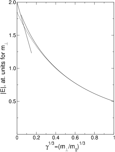
Figure 1: Binding energy of electron in an elliptical valley with the transverse to longitudinal mass ratio $\gamma$. Solid curve — result of numerical computations of the present paper. Dashed curve — result of variational fit with the trial function (26). Solid straight line — approximate adiabatic solution (27) near $\gamma=0$.

Before proceeding to calculation of exchange interaction between elliptic valleys we first remind several details about single-electron ground state that will be important for the calculation. Ground state energy spans the interval changing from $-2$ to $-\frac{1}{2}$ when $\gamma$ ranges from 0 to 1 (see Fig. 1). $\gamma=1$ corresponds to the spherical symmetric case with the ground state energy $E_{t}=-\frac{1}{2}$ of a hydrogen-like center. For $\gamma<1$ ground state energy was calculated in kohn55 by variational two-parameter fit with the trial function

$$\varphi_{\mathrm{var}}=(\pi a_{\perp}^{2}a_{\parallel})^{-1/2}e^{-\sqrt{\rho^{2}/a_{\perp}^{2}+z^{2}/a_{\parallel}^{2}}}$$ (26)

(dashed curve in Fig. 1).

Our results of numerical calculations by the method of differential sweeping in an infinite interval with singularity abramov81 are presented in Fig. 1 as solid curve. The wave function was sought in the form of the expansion in $L=40$ first Legendre polynomials in polar angle $\theta$ with respect to the axis $\hat{\mathbf{d}}_{u}$. The cut-off at $L=40$ of the indefinite basis cannot affect noticeably the accuracy of calculations until the ratio of characteristic longitudinal and transverse length scales $\gamma^{1/2}$ becomes comparable or less than the minimal scale $\sim L^{-1}$ of the truncated basis. For that reason we have not plotted the numerical curve $E_{\parallel}(\gamma)$ down to $\gamma\to 0$, where larger and larger basis would be required. However, an approximate solution may be found in an adiabatic approach kohn55 :

$$E_{\parallel}\approx-2-4\alpha^{\prime}_{0}\sqrt[3]{2\gamma},$$ (27)

where $\alpha^{\prime}_{0}\approx-1.02$ is the first root of the derivative $\mathrm{Ai}^{\prime}$ of the Airy function. This expression is shown in Fig. 1 as solid straight line.

At large distances from impurity the wave function of a localized state with $E_{\parallel}=-\alpha^{2}/2$ asymptotically falls off as

$$\varphi\approx A(\theta)\widetilde{r}^{q/\alpha-1}e^{-\alpha\widetilde{r}},$$ (28)

where $\widetilde{r}=|\widetilde{r_{i}}|$, $\widetilde{r_{i}}=D_{ij}^{-1/2}r_{j}$ and $D_{ij}^{-1/2}=(\delta_{ij}-\hat{d}_{i}\hat{d}_{j})+\gamma^{-1/2}\hat{d}_{i}\hat{d}_{j}$. We introduced

$$q^{2}(\theta)\equiv D_{ij}^{-1}\hat{\zeta}_{i}\hat{\zeta}_{j}=\sin^{2}\theta+\gamma^{-1}\cos^{2}\theta,$$ (29)

where $\theta$ is the angle between $\hat{\mbox{\boldmath$\zeta$}}$ and $\hat{\mathbf{d}}$.

In real semiconductors several degenerate elliptic valleys with different $\hat{\mathbf{d}}_{u}$ ($\hat{\mathbf{d}}_{u}$ along the rotation axis of the ellipsoid) contribute, generally speaking, to the wave function and hence to the exchange energy. Before addressing the complications due to the valley degeneracy, consider first two donors in a hypothetic tetragonal semiconductor with only one elliptic valley allowed by symmetry. We assume again the two-electron wave function to have the form (14), where, however, the two single-electron functions $\varphi_{\nu_{\mathrm{A}}}(\mathbf{r}_{1\mathrm{A}})$, $\varphi_{\nu_{\mathrm{B}}}(\mathbf{r}_{2\mathrm{B}})$ should now be found from solution of the Schrödinger equation for an elliptic valley. Proceeding as above, from a bilinear kinetic energy $D_{ij}\partial_{i}\partial_{j}$ we obtain instead of Eq. (15)

$$\Bigl{[}-\left(D_{1ij}\frac{\partial_{1i}\varphi_{\mathrm{A}}}{\varphi_{\mathrm{A}}}\partial_{1j}+D_{2ij}\frac{\partial_{2i}\varphi_{\mathrm{B}}}{\varphi_{\mathrm{B}}}\partial_{2j}\right) -$$ (30)

$$-\frac{1}{R/2-\zeta_{1}}-\frac{1}{R/2+\zeta_{2}}+\frac{1}{R}+\frac{1}{r_{12}}\Bigr{]}\chi = 0.$$

At large distances $\mathbf{r}\approx\zeta\hat{\mbox{\boldmath$\zeta$}}$ along the $\hat{\mbox{\boldmath$\zeta$}}$-direction $\widetilde{r}\approx q(\theta)|\zeta|$, where $q(\theta)$is from (29), and then from (28) obtain

$$-\frac{D_{ij}\partial_{j}e^{-\alpha\widetilde{r}}}{e^{-\alpha\widetilde{r}}}=\alpha\frac{r_{i}}{\widetilde{r}}\approx\frac{\alpha}{q(\theta)}\widehat{\zeta}_{i}\mathop{\mathrm{sgn}}\nolimits\zeta.$$ (31)

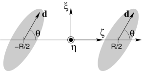
Figure 2: Frame ($\hat{\mbox{\boldmath$\xi$}},\hat{\mbox{\boldmath$\eta$}},\hat{\mbox{\boldmath$\zeta$}}$) for calculation of exchange between two elliptic valleys with the same $\hat{\mathbf{d}}$. The $\hat{\mbox{\boldmath$\zeta$}}$-axis connects the two centers.

In the coordinate system chosen the angles $\theta$ are equal for the two impurity centers (see Fig. 2). Hence (30) reduces to (15) with $\alpha\to\alpha/q(\theta)$. This substitution also gives the new expression for the matrix elements $J$ to replace (11). Also the two-electron wave functions (14) in expression (11) now contain single-electron functions corresponding to elliptic valleys.

To calculate $J$ we now follow the scheme presented in Section II for atoms. To expand the exponents in the single-electron wave functions we supplement the inter-impurity axis $\hat{\mbox{\boldmath$\zeta$}}$ with perpendicular axes $\hat{\mbox{\boldmath$\xi$}}$ and $\hat{\mbox{\boldmath$\eta$}}$ so that $\hat{\mathbf{d}}=\hat{\mbox{\boldmath$\zeta$}}\cos\theta+\hat{\mbox{\boldmath$\xi$}}\sin\theta$ and expand $\widetilde{r}$ in the small ratios $\xi/\zeta$ and $\eta/\zeta$ up to second order

$$\widetilde{r}\approx q|\zeta|\left[1+\frac{(\textstyle\frac{1}{\gamma}-1)\sin\theta\cos\theta}{q^{2}}\frac{\xi}{\zeta}+\frac{\eta^{2}}{2q^{2}\zeta^{2}}+\frac{\xi^{2}}{2\gamma q^{4}\zeta^{2}}\right].$$ (32)

Applying this expansion to the sum $\widetilde{r}_{1\mathrm{A}}+\widetilde{r}_{1\mathrm{B}}$ of the exponents we substitute $\zeta$ with $\zeta_{\pm}=\zeta\pm R/2$. Since for the electrons located between the ions $-R/2<\zeta<R/2$: $|\zeta_{\pm}|=\pm\zeta_{\pm}$, terms linear in $\xi$ in (32) cancel each other.

Hence like in atomic case we are left with the Gaussian integrals over transverse coordinates $\mbox{\boldmath$\rho$}_{1}=(\xi_{1},\eta_{1})$ and $\mbox{\boldmath$\rho$}_{2}$ that decouple from the integral over $\zeta$. By the substitution (20) the Gaussian integrals reduce to a single integral over the polar angle $\varphi_{12}$ of $\mbox{\boldmath$\rho$}_{12}$:

$$S(\theta)=\frac{1}{2\pi}\int_{0}^{2\pi}\frac{d\varphi}{\left[\sin^{2}\varphi+\cos^{2}\varphi/\gamma q^{2}\right]^{1+\frac{q}{2\alpha}}}.$$ (33)

In the spherically symmetric case $\gamma=q=1$ the integral $S(\theta)=1$.

Calculating matrix element (11) gives eventually

$$J=-(4\pi)^{2}\sqrt{\gamma}A^{4}(\theta)S(\theta)I(\alpha,q)R^{7q/2\alpha-1}e^{-2\alpha qR},$$ (34)

where

$$I(\alpha,q)=\frac{\Gamma\left(q/2\alpha\right)q^{3+q/2\alpha}}{2^{2+q/\alpha}\alpha^{2+q/2\alpha}}\int_{0}^{1}t^{3/2\alpha}(2-t)^{1/2\alpha}e^{-qt/\alpha}dt.$$ (35)

and the integration variable in (35) $t=1-2\zeta/R$. For two spherically symmetric ($\gamma=1$) atoms with angular momentum projection $m=0$ the asymptotic coefficient $A(\theta)=A/\sqrt{4\pi}$ (see (19)) and Eq. (34) reduces to (21) as it should.

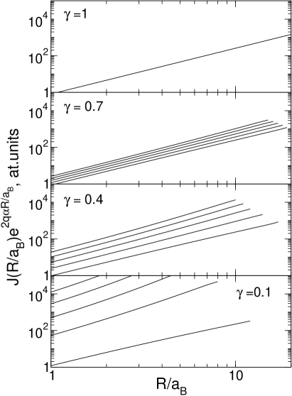
Figure 3: Preexponents of exchange integrals between ground states of electrons localized in elliptic valleys vs. donor center separation for four values of $\gamma=0.1$, 0.4, 0.7, and 1. For each value of $\gamma$ five curves are plotted for different angles between the preferred direction of the elliptic valley and the inter-center axis: $\theta=0$, $\pi/6$, $\pi/4$, $\pi/3$, $\pi/2$ (from top to bottom). In the spherical symmetric case $\gamma=1$ exchange does not depend on $\theta$.

In addition to finding the binding energy we have also carried out numerical calculation of single-electron wave functions to obtain asymptotics (28) and exchange integrals (34) using the differential sweeping method abramov81 . The preexponents of the exchange integrals, $J(R)e^{2\alpha qR}$, are presented in Fig. 3 for $\gamma=0.1$, 0.4, 0.7, and 1, and for $\theta=0$, $\pi/6$, $\pi/4$, $\pi/3$, and $\pi/2$ (from top to bottom) for each $\gamma$. In the interval of inter-center separations $1<R<10$ accessible for numerical evaluation the dependence of preexponents on $R$ is approximately linear in double logarithmic scale with the slope agreeing well with $7q/2\alpha-1$ which follows from (34).

Returning now to realistic semiconductors, recall that degenerate valleys have different anisotropic dependence for the decay of the wave function of localized electron. For an arbitrary orientation of the axis connecting two donor centers the main contribution to exchange interaction comes from the wave function components corresponding to the pair of valleys with the slowest decay, contributions of the other pairs being exponentially suppressed. In other words, among all the elements

$$\langle uv|J|u^{\prime}v^{\prime}\rangle\sim e^{-\alpha[q(\theta_{u})+q(\theta_{v})+q(\theta_{u^{\prime}})+q(\theta_{v^{\prime}})]R/2},$$ (36)

we can, with the accuracy up to exponentially small terms, keep only the elements between such states $u$ that the exponent in (36) is minimal: $\langle uu|J|uu\rangle\sim e^{-2\alpha q(\theta_{u})R}$. Therefore, for any arrangement of impurity centers except for high symmetry directions the electron exchange is predominantly caused by the overlap of the wave function components from valleys with $\hat{\mathbf{d}}_{\mathrm{A}}=\hat{\mathbf{d}}_{\mathrm{B}}$, which means that the term splitting is correctly described by Eq. (34).

The relative position of the two donors being changed, crossover between the pairs of valleys contributing the most into the exchange matrix element (36) occurs .

These considerations are not changed if one takes into account the lifting of the inter-valley degeneracy of a single center by the short-range part of the impurity potential (“central-cell correction”). The ground state in this case is the non-degenerate symmetric combination of the functions (1)kohn55

$$\psi_{g}(\mathbf{r})=\frac{1}{\sqrt{\Gamma}}\sum_{u=1}^{\Gamma}\varphi_{u}(\mathbf{r})\psi_{u}(\mathbf{r}),$$ (37)

where $\psi_{u}(\mathbf{r})\propto e^{i\mathbf{k}_{u}\mathbf{r}}$ are the Bloch functions at the minimum of the conduction band located at $\mathbf{k}=\mathbf{k}_{u}$, and $\Gamma$ is the number of the participating valleys (6 in Si, 4 in Ge, and 3 in III-V compounds).

Considering the Bloch functions oscillate rapidly on atomic scale much smaller than the effective Bohr radius, exchange interactions between the states (37) may be seen to beandres81

$$J_{g}\approx\frac{1}{\Gamma^{2}}\sum_{u,v=1}^{\Gamma}\langle uv|J|uv\rangle e^{i(\mathbf{k}_{v}-\mathbf{k}_{u})\mathbf{R}}.$$ (38)

If we average over the rapidly oscillating exponential terms, we get

$$J_{g}\approx\frac{1}{\Gamma^{2}}\sum_{u=1}^{\Gamma}\langle uu|J|uu\rangle,$$ (39)

which shows that the exchange between the symmetric ground states of multi-valley donors for any arrangement except along high symmetry directions is described by Eq. (34) with the asymptotic parameter $A(\theta)\to A(\theta)/\sqrt{\Gamma}$.

Concluding this Section, we discuss briefly the previous study of exchange interaction between donors andres81 . In the cited paper, the anisotropy of the exponential dependence of exchange interaction for elliptic valleys was completely ignored by substituting the expression for isotropic atomic exchange. Whereas, e.g., for Si $\gamma=m_{\bot}/m_{\parallel}\approx 0.21$, and hence $q(\theta)$ (29) in the exponent of the exchange interaction $\propto e^{2\alpha q(\theta)R}$ changes from $\gamma^{-1/2}\approx 2.2$ for $\theta=0$ to $0$ for $\theta=\pi/2$. Besides, in Ref. andres81 the Heitler-London approximation was used, the approach proved incorrect in calculating the preexponential factors at large distances. On the other hand, we obtained exact asymptotic expressions for the dependence of the exchange interaction on the valley parameter $\gamma$ and the mutual orientation of donors $\theta$.

IV Asymmetric exchange interaction (donors)

In semiconductors without center of inversion symmetry, such as III-V or II-VI compounds, spin-orbital interaction for donors acquires the form dresselhaus55 ; DP

$$\hat{\mathcal{H}}_{\mathrm{so}}=\mathbf{h}(-i\mbox{\boldmath$\partial$})\hat{\mathbf{s}}.$$ (40)

Wave function of a single electron cannot be represented as a product of spin and coordinate components any more. An approach with the expansion (6) is nevertheless applicable after suitable adjustments gorkov03 .

In the presence of spin-orbital Hamiltonian (40) spin projection no longer commutes with the total Hamiltonian, but the two-fold (Kramers) degeneracy of the ground state remains. Index numbering this degeneracy may be included into the full set $\nu$ of indices describing a single-electron state. The permutation operator $\hat{P}$ in (6) now interchanges both spin and coordinate variables of the electrons.

Correspondingly, the provision for the total wave function $\psi$ (6) to be antisymmetric in electron permutation: $\psi=-\hat{P\psi}$, leads to $c_{\nu_{\mathrm{A}}\nu_{\mathrm{B}}}=-c_{\nu_{\mathrm{A}}\nu_{\mathrm{B}}}^{(P)}$.

For simplicity we will restrict ourselves to donors in II-VI and III-V semiconductors where besides being a Kramers doublet single-electron state on a donor is not otherwise degenerate. Then $\nu$ will stand for the Kramers index.

In bulk zinc-blende semiconductors dresselhaus55 ; DP

$$h_{x}(\mathbf{k})=\frac{\alpha_{\mathrm{so}}}{\sqrt{2E_{g}}}k_{x}(k_{y}^{2}-k_{z}^{2})$$ (41)

and $h_{y}(\mathbf{k})$ and $h_{z}(\mathbf{k})$ are obtained by permutation in (41). Here $E_{g}$ is the band gap in atomic units and $\alpha_{\mathrm{so}}$ is a phenomenological parameter. For GaAs $E_{g}\approx 1.43$ eV (in atomic units this yields $E_{g}\approx 113$ under the radical sign in (41)) and $\alpha_{\mathrm{so}}\approx 0.07$.

For small spin-orbital interaction the spinor single-electron wave functions are

$$\varphi_{\nu}^{\beta}(\mathbf{r})\approx\varphi_{0}(r)(e^{i\alpha^{2}\mathbf{h}(\hat{\mathbf{r}})r\mbox{\scriptsize\boldmath$\sigma$}/2})^{\beta\nu},$$ (42)

where $\varphi_{0}(r)=e^{-r}/\sqrt{\pi}$ is the hydrogenic ground state wavefunction and $\hat{\mathbf{r}}=\mathbf{r}/r$. The phase factor turns into unity when $r\to 0$. Thus the Kramers index takes on the meaning of the spin projection of an electron on the center $\nu=\uparrow,\downarrow$.

Two-electron wave functions have now to be sought as solutions of the Hamiltonian

$$\hat{\mathcal{H}} = -\textstyle\frac{1}{2}\mbox{\boldmath$\partial$}_{1}^{2}-\textstyle\frac{1}{2}\mbox{\boldmath$\partial$}_{2}^{2}+\hat{\mathcal{H}}_{\mathrm{so}1}+\hat{\mathcal{H}}_{\mathrm{so}2}-1/r_{1\mathrm{A}}-1/r_{2\mathrm{B}}$$ (43)

$$- 1/r_{2\mathrm{A}}-1/r_{1\mathrm{B}}+1/r_{12}+1/R.$$

in the form (17)

$$\psi_{\nu_{\mathrm{A}}\nu_{\mathrm{B}}}^{\alpha\beta}(\mathbf{r}_{1},\mathbf{r}_{2})=\chi^{\alpha\alpha^{\prime},\beta\beta^{\prime}}(\mathbf{r}_{1},\mathbf{r}_{2})\varphi_{\nu_{\mathrm{A}}}^{\alpha^{\prime}}(\mathbf{r}_{1\mathrm{A}})\varphi_{\nu_{\mathrm{B}}}^{\beta^{\prime}}(\mathbf{r}_{2\mathrm{B}}),$$ (44)

with $\chi^{\alpha\alpha^{\prime},\beta\beta^{\prime}}$converting to $\delta^{\alpha\alpha^{\prime}}\delta^{\beta\beta^{\prime}}$ when either $\mathbf{r}_{1\mathrm{A}}\to 0$ or $\mathbf{r}_{2\mathrm{B}}\to 0$. The principal terms in spin-orbital interaction are included into definition (42), and the equation for $\chi^{\alpha\alpha^{\prime},\beta\beta^{\prime}}$ turns out to coincide with (15). Therefore $\chi^{\alpha\alpha^{\prime},\beta\beta^{\prime}}=\chi\delta^{\alpha\alpha^{\prime}}\delta^{\beta\beta^{\prime}}$ with $\chi$ from (14).

Similarly to (10) we get

$$(E-E_{0})c_{\nu_{\mathrm{A}}\nu_{\mathrm{B}}}=\sum_{\nu^{\prime}_{\mathrm{A}}\nu^{\prime}_{\mathrm{B}}}J_{\nu_{\mathrm{A}}\nu_{\mathrm{B}}\nu^{\prime}_{\mathrm{A}}\nu^{\prime}_{\mathrm{B}}}c_{\nu^{\prime}_{\mathrm{A}}\nu^{\prime}_{\mathrm{B}}}^{(P)},$$ (45)

where

$$J_{\nu_{\mathrm{A}}\nu_{\mathrm{B}}\nu^{\prime}_{\mathrm{A}}\nu^{\prime}_{\mathrm{B}}} = -2\int_{\zeta_{1}=\zeta_{2}}\psi_{\nu_{\mathrm{A}}\nu_{\mathrm{B}}}^{*}\psi_{\nu^{\prime}_{\mathrm{B}}\nu^{\prime}_{\mathrm{A}}}d\zeta d^{4}\mbox{\boldmath$\rho$}_{1,2}$$ (46)

$$= J(R)(e^{-i\mbox{\scriptsize\boldmath$\gamma$}\mbox{\scriptsize\boldmath$\sigma$}/2})_{\nu_{\mathrm{A}}\nu^{\prime}_{\mathrm{B}}}(e^{i\mbox{\scriptsize\boldmath$\gamma$}\mbox{\scriptsize\boldmath$\sigma$}/2})_{\nu_{\mathrm{B}}\nu^{\prime}_{\mathrm{A}}}.$$

The exchange integral $J(R)=-0.818R^{5/2}e^{-2R}$ gorkov64 ; herring64 and

$$\mbox{\boldmath$\gamma$}=\mathbf{h}(\hat{\mbox{\boldmath$\zeta$}})R..$$ (47)

Absolute value $|\mbox{\boldmath$\gamma$}|/2$ plays the role of angle of rotation of electron spin around the axis $\hat{\mbox{\boldmath$\gamma$}}$ when it tunnels between each of the centers A and B and the median plane. Using

$$c_{\nu_{\mathrm{A}}\nu_{\mathrm{B}}}^{(P)}=-c_{\nu_{\mathrm{A}}\nu_{\mathrm{B}}}\equiv-\textstyle\frac{1}{2}(\mbox{\boldmath$\sigma$}_{\nu_{\mathrm{A}}\nu^{\prime}_{\mathrm{A}}}\mbox{\boldmath$\sigma$}_{\nu_{\mathrm{B}}\nu^{\prime}_{\mathrm{B}}}+\delta_{\nu_{\mathrm{A}}\nu^{\prime}_{\mathrm{A}}}\delta_{\nu_{\mathrm{B}}\nu^{\prime}_{\mathrm{B}}})c_{\nu^{\prime}_{\mathrm{B}}\nu^{\prime}_{\mathrm{A}}}.$$ (48)

we finally arrive at the equation $(E-E_{0})c=\hat{\mathcal{H}}_{\mathrm{ex}}c$ for the coefficients $c_{\nu_{\mathrm{A}}\nu_{\mathrm{B}}}$, with the Hamiltonian gorkov03

$$\hat{\mathcal{H}}_{\mathrm{ex}} = -\textstyle\frac{1}{2}Je^{-i\mbox{\scriptsize\boldmath$\gamma$}(\mbox{\scriptsize\boldmath$\sigma$}_{1}-\mbox{\scriptsize\boldmath$\sigma$}_{2})/2}\left(\hat{\mbox{\boldmath$\sigma$}}_{1}\hat{\mbox{\boldmath$\sigma$}}_{2}+1\right)$$

$$\equiv -\textstyle\frac{1}{2}J\left[\hat{\mbox{\boldmath$\sigma$}}_{1}\overleftrightarrow{R}(\mbox{\boldmath$\gamma$})\hat{\mbox{\boldmath$\sigma$}}_{2}+1\right]$$

$$\approx -\textstyle\frac{1}{2}J\left[\hat{\mbox{\boldmath$\sigma$}}_{1}\hat{\mbox{\boldmath$\sigma$}}_{2}+1-\mbox{\boldmath$\gamma$}\left(\hat{\mbox{\boldmath$\sigma$}}_{1}\times\hat{\mbox{\boldmath$\sigma$}}_{2}\right)\right],$$

where the Pauli matrices $\hat{\mbox{\boldmath$\sigma$}}_{1}$ and $\hat{\mbox{\boldmath$\sigma$}}_{2}$ act in the space of the Kramers indices, and $\overleftrightarrow{R}(\mbox{\boldmath$\gamma$})$ is the three-dimensional rotation matrix on the angle $\gamma$ around the axis $\hat{\mbox{\boldmath$\gamma$}}$.

In the absence of spin-orbital interaction (40) the angle $|\mbox{\boldmath$\gamma$}|=0$ and we return to the exchange Hamiltonian (5) as expected.

In this Section we have considered the expansion of spin-orbital interaction (40) in bulk III-V semiconductors, where (40) begins with the third power in momentum. Analogously, one can study spin-orbital interaction linear in momentum which appears in reduced symmetry or dimensionality (in films or at the surface). All the derivation including the expression (47) for angle $\gamma$ remains intact. The case of linear spin-orbital interaction has also been studied differently in Ref. kavokin03 .

V Degenerate bands (acceptors)

As we will see later, calculation of the exchange interaction between two shallow acceptor centers has much in common with the problem of two hydrogen atoms each in a state with non-zero momentum discussed in Section II and in the Appendix. However, the analogy is not complete, the calculations become laborious and we have not performed them fully. In what follows we only determine the sign of the exchange interaction. More precisely, it is shown that the magnetic moment in the ground state of a pair of acceptors equals zero.

We begin this Section by first reviewing the properties of a single acceptor center.

Without taking spin-orbital interaction into account the valent band of typical semiconductors (Ge, Si, III-V) would be six-fold degenerate at the point $\mathbf{k}=0$. Spin-orbital interaction splits the valent band into a two- and four-fold degenerate bands separated by a gap. If the spin-orbital splitting is large with respect to the binding energy of an acceptor, the two-fold degenerate band can be neglected. For $\mathbf{k}\neq 0$ the four-fold degeneracy of the upper-lying band is lifted and two two-fold bands of light and heavy holes are formed. Their energy spectrum $\epsilon(\mathbf{k})$ quadratic in $k$ is known to depend on the direction of the quasimomentum $\hat{\mathbf{k}}$ through three invariants of the $O_{h}$ point symmetry group so that surfaces $\epsilon(\mathbf{k})=\mathop{\mathrm{const}}\nolimits$ are slightly warped spheres.

As is known, the spectrum in the vicinity of $\mathbf{k}=0$ is determined by three Luttinger parameters $\gamma_{1}$, $\gamma_{2}$ and $\gamma_{3}$. In practice, two of them are close $\gamma_{2}\approx\gamma_{3}=\overline{\gamma}$ and the dispersion relation is simply $\epsilon=k^{2}/2m_{l,h}$, where $m_{l,h}=m_{0}/(\gamma_{1}\pm\overline{\gamma})$ are the effective masses of the light and heavy holes. In this so called spherical approximation the Schrödinger equation for the four-component envelope hole wave function $\varphi^{\alpha}$ is given by (2) with the effective mass tensor

$$D_{ij}=\frac{1}{m_{0}}\left[\gamma_{1}\delta_{ij}-\overline{\gamma}\left(\{J_{i}J_{j}\}-\textstyle\frac{1}{3}\mathbf{J}^{2}\delta_{ij}\right)\right],$$ (50)

where $\mathbf{J}$ is the 4$\times$4 matrix of the pseudospin operator $J=\frac{3}{2}$ and $\{J_{i}J_{j}\}=\frac{1}{2}(J_{i}J_{j}+J_{j}J_{i})$.

It is convenient to rewrite (50) using atomic units $a_{\mathrm{B}}=\kappa/m_{h}e^{2}$ and $2\mathrm{Ry}=1/m_{h}a_{\mathrm{B}}^{2}$:

$$D_{ij}=\frac{1}{1-\mu}\left[\delta_{ij}-\mu\left(\{J_{i}J_{j}\}-\textstyle\frac{1}{3}\mathbf{J}^{2}\delta_{ij}\right)\right].$$ (51)

Here

$$\mu=\frac{\overline{\gamma}}{\gamma_{1}}=\frac{m_{h}-m_{l}}{m_{h}+m_{l}}.$$ (52)

In the limit of equal masses $m_{h}$ and $m_{l}$ the four components of $\varphi^{\alpha}$ in (2) decouple, each satisfying the Schrödinger equation for a hydrogen atom with the ground state energy $E_{h}=-1/2$ for orbital momentum $L=0$. In the general case $m_{h}>m_{l}$ acceptor states may be classified lipari70 ; gel'mont71 ; baldereschi73 by the total angular momentum $\mathbf{F}=\mathbf{J}+\mathbf{L}$ and its projection $m_{F}$:

$$|Fm_{F}\rangle=\sum_{L}\sum_{m_{J},m_{L}}\langle m_{J}m_{L}|Fm_{F}\rangle|Jm_{J}\rangle|Lm_{L}\rangle,$$ (53)

where $\langle m_{J}m_{L}|Fm_{F}\rangle$ are the Clebsh-Gordan coefficients and $m_{J}+m_{L}=m_{F}$, $|Lm_{L}\rangle=R_{L}(r)Y_{L}^{m_{L}}(\hat{\mathbf{r}})$, $Y_{L}^{m_{L}}(\hat{\mathbf{r}})$ are the spherical harmonics and $|Jm_{J}\rangle$ is a column in the pseudospin index with one non-zero component at $m_{J}$. The summation over $L$ for a given $F$ runs over all such values that $|L-J|\leq F\leq L+J$.

Substituting (53) into (2) with (51) results in the Sturm-Liouville problem on the energy $E_{h}$ and the unknown radial functions $R_{L}(r)$. The ground state turns out to be four-fold degenerate with $F=\frac{3}{2}$ (It is, in fact, the only state with possible $L=0$, hence it becomes the correct ground state in the limit $m_{h}=m_{l}$). In this state only the radial functions $R_{L}(r)$ with $L=0$ and 2 turn out to be coupled:

$$\left(\begin{array}[]{cc}\partial_{r}^{2}+\frac{2}{r}\partial_{r}&-\mu\left(\partial_{r}^{2}+\frac{5}{r}\partial_{r}+\frac{3}{r^{2}}\right)\\ -\mu\left(\partial_{r}^{2}-\frac{1}{r}\partial_{r}\right)&\partial_{r}^{2}+\frac{2}{r}\partial_{r}-\frac{6}{r^{2}}\end{array}\right)\left({R_{0}\atop R_{2}}\right)$$ (56)

$$+2(1-\mu)\left(E_{h}+\textstyle\frac{1}{r}\right)\left({R_{0}\atop R_{2}}\right) = 0$$

Numerical solution gel'mont71 of this equation shows that $E_{h}$ changes from $-\frac{1}{2}$ at $\mu=0$ ($m_{h}=m_{l}$) to $\approx-\frac{2}{9}$ in the limit $\mu\to 1$ ($m_{h}\gg m_{l}$). Thus the binding energy is determined by the scale of the heavy mass. At large $r$ (56) yields

$$(1-\mu)(\partial_{r}^{2}+2E_{h})(R_{0}+R_{2}) = 0,$$ (57)

$$(\partial_{r}^{2}+2E_{h}m_{l}/m_{h})(R_{0}-R_{2}) = 0,$$ (58)

which shows that for $m_{h}\gg m_{l}$ the sum of the two functions falls off on the scale $1/\sqrt{2|E_{h}|}$ corresponding to the heavy holes, i.e. much faster than their difference, falling off on the scale determined by the light holes. Then at large $r$ shklovskii84 $R_{0}\approx-R_{2}\propto e^{-\alpha_{l}r}$ with

$$\alpha_{l}=\sqrt{2|E_{h}|m_{l}/m_{h}}.$$ (59)

The four degenerate wave functions of the ground state (53) in the asymptotic region close to the axis $\hat{\mbox{\boldmath$\zeta$}}$ connecting the impurities (chosen as the quantization axis for the orbital momentum $\mathbf{L}$) are

$$\varphi_{\frac{3}{2}}(\mathbf{r}) = -R_{0}(r)\sqrt{\frac{3}{4\pi}}\theta e^{i\varphi}|\textstyle\frac{1}{2}\rangle,$$

$$\varphi_{\frac{1}{2}}(\mathbf{r}) = \frac{R_{0}(r)}{\sqrt{\pi}}\left(|\textstyle\frac{1}{2}\rangle-\frac{\sqrt{3}}{2}\theta e^{-i\varphi}|\textstyle\frac{3}{2}\rangle\right),$$ (60)

$$\varphi_{-\frac{1}{2}}(\mathbf{r}) = \frac{R_{0}(r)}{\sqrt{\pi}}\left(|\textstyle-\frac{1}{2}\rangle+\frac{\sqrt{3}}{2}\theta e^{i\varphi}|\textstyle-\frac{3}{2}\rangle\right),$$

$$\varphi_{-\frac{3}{2}}(\mathbf{r}) = R_{0}(r)\sqrt{\frac{3}{4\pi}}\theta e^{-i\varphi}|\textstyle-\frac{1}{2}\rangle.$$

Here the four unit columns $|Jm_{J}\rangle=|\pm 3/2\rangle$, $|\pm 1/2\rangle$ form the basis in the pseudo-spin $3/2$ space, and we have left only terms up to first order in the small polar angle $\theta$ (cf. Eq. (18)).

Proceeding now to the calculation of exchange interaction, we construct asymptotically correct basis of the direct product of the ground states on two centers in the form

$$\psi_{m_{F}^{\mathrm{A}}m_{F}^{\mathrm{B}}}^{\alpha\beta}(\mathbf{r}_{1},\mathbf{r}_{2})=\chi^{\alpha\gamma,\beta\delta}(\mathbf{r}_{1},\mathbf{r}_{2})\varphi_{m_{F}^{\mathrm{A}}}^{\gamma}(\mathbf{r}_{1\mathrm{A}})\varphi_{m_{F}^{\mathrm{B}}}^{\delta}(\mathbf{r}_{2\mathrm{B}}).$$ (61)

The total two-electron wave function $\psi$ is again sought in the form (6), where the condition $c_{m_{F}^{\mathrm{A}}m_{F}^{\mathrm{B}}}=-c_{m_{F}^{\mathrm{A}}m_{F}^{\mathrm{B}}}^{(P)}$ is required for the wave function $\psi$ to be antisymmetric in particle permutation. Equation on $\chi$ is obtained by substitution of this form into the two-hole Hamiltonian:

$$\alpha_{l}(D_{ij}^{\alpha\alpha^{\prime}}\hat{\zeta}_{i}\partial_{1j}\chi^{\alpha^{\prime}\gamma,\beta\delta}-D_{ij}^{\beta\beta^{\prime}}\hat{\zeta}_{i}\partial_{2j}\chi^{\alpha\gamma,\beta^{\prime}\delta}) +$$

$$+\Bigl{[}-\frac{1}{R/2-\zeta_{1}}-\frac{1}{R/2+\zeta_{2}}+\frac{1}{R}+\frac{1}{r_{12}}\Bigr{]}\chi^{\alpha\gamma,\beta\delta} = 0,$$ (62)

where we used the asymptotics $\partial_{i}\varphi\approx-\alpha_{l}\varphi\partial_{i}r=-\alpha_{l}\varphi\hat{\zeta}_{i}\mathop{\mathrm{sgn}}\nolimits\zeta$ at large $\mathbf{r}=\hat{\mbox{\boldmath$\zeta$}}|\zeta|$ (cf. (30)).

We neglect the derivatives of $\chi$ over transverse coordinates as they are, as before, of higher order in $1/R$ (the validity of this approximation is verified by differentiating the resulting expression for $\chi$).

Moreover, in the spherical approximation we consider, the hole Hamiltonian is invariant under transformations from the spherical point symmetry group $K_{h}$ and not only from $O_{h}$. Therefore, in this approximation, axis $\hat{\mbox{\boldmath$\zeta$}}$ connecting the acceptor centers may be chosen as the quantization axis of the moments $\mathbf{J}$, $\mathbf{L}$ and $\mathbf{F}$, and the problem acquires some resemblance with the hydrogen problem studied in Section I.

In particular, the equations (62) on $\chi$ decouple from each other:

$$\alpha_{l}(D_{zz}^{\alpha\alpha^{\prime}}\partial_{\zeta_{1}}\chi^{\alpha^{\prime}\gamma,\beta\delta}-D_{zz}^{\beta\beta^{\prime}}\partial_{\zeta_{2}}\chi^{\alpha\gamma,\beta^{\prime}\delta}) +$$

$$+\Bigl{[}-\frac{1}{R/2-\zeta_{1}}-\frac{1}{R/2+\zeta_{2}}+\frac{1}{R}+\frac{1}{r_{12}}\Bigr{]}\chi^{\alpha\gamma,\beta\delta} = 0,$$ (63)

because matrices $D_{zz}^{\alpha\alpha^{\prime}}$ and $D_{zz}^{\beta\beta^{\prime}}$ are diagonal:

$$D_{zz}=\left(\begin{array}[]{cccc}1&0&0&0\\ 0&m_{h}/m_{l}&0&0\\ 0&0&m_{h}/m_{l}&0\\ 0&0&0&1\end{array}\right),$$

as can be easily seen using the explicit form of the pseudo-spin matrix $J_{z}$. Together with the boundary condition $\chi^{\alpha\gamma,\beta\delta}{}\to\delta^{\alpha\gamma}\delta^{\beta\delta}$ when either $\mathbf{r}_{1}\to-\mathbf{R}/2$ or $\mathbf{r}_{2}\to\mathbf{R}/2$, this equation yields solution for $\chi^{\alpha\gamma,\beta\delta}$ diagonal in each pair of band indices. i.e. only the elements with $\alpha=\gamma$, $\beta=\delta$ are non-zero.

Because of such diagonal structure, the one-hole functions in the elements of the exchange integral matrix

$$J_{m_{F}^{\mathrm{A}}m_{F}^{\mathrm{B}}m_{F}^{\mathrm{A}}{}^{\prime}m_{F}^{\mathrm{B}}{}^{\prime}}=-2\alpha_{l}\sum_{\alpha\beta}\int_{\zeta_{1}=\zeta_{2}}\left(\chi^{\alpha\alpha,\beta\beta}\right)^{2}$$ (64)

$$\times\varphi_{m_{F}^{\mathrm{A}}}^{\alpha}(\mathbf{r}_{1\mathrm{A}})\varphi_{m_{F}^{\mathrm{B}}}^{\beta}(\mathbf{r}_{2\mathrm{B}})\varphi_{m_{F}^{\mathrm{A}}{}^{\prime}}^{\alpha}(\mathbf{r}_{2\mathrm{A}})\varphi_{m_{F}^{\mathrm{B}}{}^{\prime}}^{\beta}(\mathbf{r}_{1\mathrm{B}})d\zeta d^{4}\mbox{\boldmath$\rho$}_{1,2}.$$

At integrating wave functions (60) over transverse coordinates in (64) each $\theta$ will produce an additional smallness $R^{-1/2}$ as we have seen in Section I. In principal order we may hence leave only functions $\varphi_{\pm\frac{1}{2}}(\mathbf{r})\approx R_{0}(r)|\textstyle\pm\frac{1}{2}\rangle/\sqrt{\pi}$ (each of them has also only one non-zero pseudospin component).

The 16$\times$16 diagonal matrices $D_{zz}^{\alpha\alpha^{\prime}}\delta^{\beta\beta^{\prime}}$ before $\partial_{\zeta_{1}}$ and $\delta^{\alpha\alpha^{\prime}}D_{zz}^{\beta\beta^{\prime}}$ before $\partial_{\zeta_{2}}$ in (63) do not generally coincide for $\alpha\neq\beta$, and hence equations for all the elements of $\chi$ cannot be simply solved in terms of $\zeta_{12}$ as was done in atomic case. Nevertheless, to calculate (64) in main order we only need $\varphi_{\pm\frac{1}{2}}$ as we explained above. Equations (63) on $\chi$ for the components $\varphi_{\pm\frac{1}{2}}$ do reduce to (15) with $\alpha\to\alpha_{l}m_{h}/m_{l}$. We thus arrive to a complete analogy with the problem of exchange between two hydrogenic centers in the ground state, i.e. degenerate only over projection of spin $\frac{1}{2}$. In this analogy localized wave functions are $R_{0}(r)/\sqrt{\pi}$ and the role of the projection of “spin” $\frac{1}{2}$ is played by $m_{F}$ spanning the truncated subspace $\pm\frac{1}{2}$.

We may, therefore, at once give the asymptotically correct terms: the ground state will be the “singlet”

$$\frac{1}{\sqrt{2}}(\psi+\hat{P}\psi)\frac{1}{\sqrt{2}}(\textstyle|\frac{1}{2},-\frac{1}{2}\rangle-|-\frac{1}{2},\frac{1}{2}\rangle)$$ (65)

and the excited state will be the “triplet”

$$\frac{1}{\sqrt{2}}(\psi-\hat{P}\psi)\left\{\begin{array}[]{l}|\frac{1}{2},\frac{1}{2}\rangle\\ \frac{1}{\sqrt{2}}(|\frac{1}{2},-\frac{1}{2}\rangle+|-\frac{1}{2},\frac{1}{2}\rangle)\\ |-\frac{1}{2},-\frac{1}{2}\rangle\end{array}\right.,$$ (66)

where $\psi=\chi R_{0}(r_{1\mathrm{A}})R_{0}(r_{2\mathrm{B}})/\pi$ and $\chi$ is given by (17) with $\alpha=\alpha_{l}m_{h}/m_{l}$.

Energies of the “singlet” and “triplet” states are $E_{0}\pm J(R)$ respectively, where for the exchange splitting we obtain

$$J = -\frac{m_{l}}{m_{h}}\Gamma\left(\frac{1}{2\alpha}\right)\frac{2^{\frac{3}{\alpha}-2}R^{3-\frac{1}{2\alpha}}}{\alpha^{2+\frac{1}{2\alpha}}}e^{-2\alpha R}$$ (67)

$$\times \int_{0}^{1}\frac{P^{2}\left[\frac{R}{2}(1+t)\right]P^{2}\left[\frac{R}{2}(1-t)\right]}{(1+t)^{\frac{3}{2\alpha}-2}(1-t)^{\frac{1}{2\alpha}-2}}e^{\frac{t-1}{\alpha}}dt,$$

where $P(r)$ is defined as $P(r)=R(r)e^{2\alpha R}$ with $R(r)$ from numerical solution. For two atoms, when $m_{l}=m_{h}$, $\alpha_{l}=\alpha$ and the preexponent $P(r)=Ar^{1/\alpha-1}/2$, Eq. (67) reduces to (21).

Asymptotics $R_{0}(r)\approx R_{2}(r)=R(r)$ used to obtain $J(R)$ unfortunately sets in too far ($R>10$) and we have not evaluated (67) numerically.

Similar to the hydrogen molecule problem the two states found, (65) and (66), with energies split by the amount of $2J(R)$ (67) represent only the ground and the most excited states. Energies of all the other two-center states are defined by smaller exchange integrals and will have exchange splitting $O(R^{-1}J(R))$, i.e. at large $R$ these terms will lie between the first two.

As for the magnetic moment of a single acceptor center, it is proportional to $\mathbf{F}$ with the $g$-factor malyshev97 $g\approx 0.76$. We see immediately that the ground state of two acceptor centers is non-magnetic as is the case with hydrogenic atoms and donors.

VI Role of magnetic field

To complete the above discussion, we briefly review the impact of external magnetic fields. Strong magnetic field squeezes electron wave functions in cross direction reducing their overlap. Therefore, major changes come already in exponential factors, and one may use well-known results for the asymptotic behavior of hydrogenic wave functions in magnetic fields.

Uniform magnetic field $\mathbf{H}=H\hat{\mathbf{z}}$ with the vector potential $\mathbf{A}(\mathbf{r})=\frac{1}{2}\mathbf{H}\times\mathbf{r}$ results in an additional magnetic parabolic potential in the Schrödinger equation for the ground state

$$\left[-\frac{1}{2}\mbox{\boldmath$\partial$}^{2}-\frac{1}{r}+\frac{\rho^{2}}{8}\left(\frac{a_{\mathrm{B}}}{a_{H}}\right)^{4}\right]\varphi=E_{H}\varphi,$$ (68)

where $a_{H}^{2}=\hbar c/|e|H$ is the magnetic length. In weak magnetic fields $a_{\mathrm{B}}\ll a_{H}$ magnetic potential is weak in the region of localization $r\sim a_{\mathrm{B}}$, and $E_{H}\approx-\frac{1}{2}$. High magnetic fields $a_{\mathrm{B}}\gg a_{H}$ localize an electron in the transverse directions much stronger than Coulomb potential does, and the binding energy grows logarithmically with magnetic field $E_{H}=-\frac{1}{2}\ln^{2}(a_{\mathrm{B}}/a_{H})^{2}$.

Exponential tails of localized electron wave function in magnetic field have the following form (see shklovskii84 and references therein). For a weak field ($a_{H}\gg a_{B}$) there are two asymptotic regions with different dependencies of $\varphi(r)$. Rather close to the $\hat{\mathbf{z}}$ axis, $1\ll r\ll(a_{H}/a_{B})^{2}$, wave functions fall off as

$$\varphi\propto\exp-r\left[1+\frac{\rho^{2}}{24}\left(\frac{a_{\mathrm{B}}}{a_{H}}\right)^{4}\right],$$ (69)

whereas at large $r\gg(a_{H}/a_{B})^{2}$ as

$$\varphi\propto\exp-\left[|z|+\frac{\rho^{2}}{4}\left(\frac{a_{\mathrm{B}}}{a_{H}}\right)^{2}\right].$$ (70)

In strong magnetic fields ($a_{H}\ll a_{B}$) the first asymptotic region is absent and exponential tail of the wave function is given by

$$\varphi\propto\exp-\left[|z|\ln\left(\frac{a_{\mathrm{B}}}{a_{H}}\right)^{2}+\frac{\rho^{2}}{4}\left(\frac{a_{\mathrm{B}}}{a_{H}}\right)^{2}\right].$$ (71)

The change in the “longitudinal” asymptotics (field along the direction connecting two centers) compared to (70) is due to the change of the binding energy (and hence, of the localization length) with magnetic field.

From these formulas we observe that application of magnetic field parallel to the inter-center axis does not change the form of the exponential dependence of exchange integrals. At the same time, field perpendicular to the axis changes exponential asymptotics either to slightly corrected atomic one

$$e^{-2R(1+R^{2}(a_{B}/a_{H})^{2}/6)}$$ (72)

for $1\ll R\ll(a_{H}/a_{B}^{2})$ in weak fields, or to

$$e^{-R^{2}(a_{B}/a_{H})^{2}}$$ (73)

for $R\gg(a_{H}/a_{B}^{2})$ in weak fields and for all $R\gg 1$ in strong fields.

We conclude that magnetic field drastically changes already the exponential dependencies, and we thus will not study the behavior of the pre-exponential factors.

VII Summary

We have calculated exact asymptotic form of exchange interaction between shallow impurity centers in semiconductors at large separations generalizing the methods of the theory of hydrogenic molecules.

We found that the ground state of a pair of impurity centers is always non-magnetic. In other words, the exchange interactions between centers have the “antiferromagnetic” sign.

The essence of the method that we use is the construction of a secular equation with the matrix comprising exchange integrals between all the degenerate single-center states. The exchange integrals are expressed as the probability current through the hyperplane in the coordinate space of two electrons that separates two regions of their localization on the centers. The exchange integrals are calculated with wave functions at the hyperplane corrected for the Coulomb interaction between electrons and alien ions in principal order in inverse inter-center separation $R^{-1}$.

Exchange integrals between different degenerate single-center states may have different order in $R^{-1}$. The main exchange integrals define the energy of the lowest and the highest split terms with the remaining terms lying in between. To calculate the latter the exchange integrals in the next approximation would be necessary. However, the procedure simplifies for atoms if one uses symmetry considerations to restrict the basis of degenerate states on each center to only those that are allowed by symmetry to convert to a given term.

In semiconductors we have considered degeneracy of single-center states both in valley index (donors) and in the band spectrum near $\mathbf{k}=0$ (acceptors). For electrons localized on donors calculation of exchange interaction reduces to evaluation of exchange integrals between the components of the wave functions from different pairs of valleys. Depending on the relative position of the two donors in the cubic lattice, crossover from one pair of valleys to another takes place at high-symmetry directions. The dependence of exchange integrals on valley parameters and on the orientation of the valleys with respect to the axis connecting the two centers was calculated numerically.

We have also evaluated the asymptotic form of the asymmetric (Dzyaloshinskii-Moriya) exchange interaction for donors.

The problem of exchange interaction between two acceptors simplifies considerably in the spherical approximation when it acquires resemblance with hydrogenic molecules. We have developed the complete procedure for calculation of exchange in spherical approximation, but have restricted ourselves to the sign of the interaction only. As in the case of a hydrogen molecule, the ground state of a pair of acceptors turned out to be non-magnetic. For a detailed calculation of the exchange interaction numerical solution of the wave equation of an acceptor center at very large distances would be required, which was not possible to do in the numerical scheme we used.

The influence of external magnetic field on the strength of exchange interaction was also briefly discussed. Expectedly, magnetic field affects already the exponential dependence due to stronger localization of electron on a center in the presence of magnetic field.

VIII Acknowledgments

We are thankful to Dr. Sh. Kogan for referring us to the computational method used to find asymptotics of wave functions numerically, to Dr. B. L. Gel’mont for useful discussions, and to Dr. K. V. Kavokin for referring us to malyshev97 . The work was supported (LPG) by the NHMFL through the NSF cooperative agreement DMR-9527035 and the State of Florida, and (PLK) by DARPA through the Naval Research Laboratory Grant No. N00173-00-1-6005.

Appendix A Hierarchic structure of molecular terms

In this Appendix we present asymptotic expressions for exchange integrals between higher orbital momentum $l$ atomic states. Preexponents of these integrals contain $R$ in different degrees dependent on the projections $m$ of $l$ for the two atoms. We show how exchange integrals (and hence electronic terms) of higher than leading order in $R^{-1}$ may be found by restricting the basis of single-atom wave functions to only those allowed by symmetry to participate in a given molecular term.

The matrix elements (11) for arbitrary $l$ were considered in Ref. hadinger93 in the most general case of different binding energies of the two atoms. However, these general formulas were cumbersome and were not brought to explicit answer . Below we cite our results for the case of equal binding energies:

$$J_{\nu_{\mathrm{A}}\nu_{\mathrm{B}}\nu^{\prime}_{\mathrm{A}}\nu^{\prime}_{\mathrm{B}}} = -\left(I_{\alpha+}+I_{\alpha-}\right)A_{\nu_{\mathrm{A}}}^{*}A_{\nu_{\mathrm{B}}}^{*}A_{\nu^{\prime}_{\mathrm{A}}}A_{\nu^{\prime}_{\mathrm{B}}}$$ (74)

$$\times R^{\frac{7}{2\alpha}-1-\frac{m_{+}}{2}}e^{-2\alpha R},$$

where

$$I_{\alpha\pm} = \frac{\Gamma\left(1/2\alpha\right)}{2^{3+\frac{1}{\alpha}-\frac{m_{+}}{2}}\alpha^{2+\frac{1}{2\alpha}+\frac{m_{+}}{2}}}K(2\alpha,m_{1},m_{2},\Delta m)$$ (75)

$$\times \int_{0}^{1}(1-y)^{\frac{3}{2\alpha}\pm\frac{m_{-}}{2}}(1+y)^{\frac{1}{2\alpha}\mp\frac{m_{-}}{2}}e^{\frac{y-1}{\alpha}}dy$$

and

$$m_{+} = |m_{\mathrm{A}}|+|m^{\prime}_{\mathrm{A}}|+|m_{\mathrm{B}}|+|m^{\prime}_{\mathrm{B}}|$$

$$m_{-} = |m_{\mathrm{A}}|+|m^{\prime}_{\mathrm{A}}|-\left(|m_{\mathrm{B}}|+|m^{\prime}_{\mathrm{B}}|\right),$$

$$m_{1} = |m_{\mathrm{A}}|+|m^{\prime}_{\mathrm{B}}|,$$

$$m_{2} = |m^{\prime}_{\mathrm{A}}|+|m_{\mathrm{B}}|,$$

$$\Delta m = |m_{\mathrm{A}}-m^{\prime}_{\mathrm{B}}|.$$ (76)

The four-fold integral

$$K (2\alpha,m_{1},m_{2},\Delta m)=\frac{2\alpha}{\pi^{2}2^{1/2\alpha}\Gamma\left(1/2\alpha\right)}\int\rho_{12}^{1/\alpha}\rho_{1}^{m_{1}}\rho_{2}^{m_{2}}$$ (77)

$$\times e^{-\rho_{1}^{2}-\rho_{2}^{2}}\cos\left[\Delta m(\varphi_{1}-\varphi_{2})\right]d^{2}\mbox{\boldmath$\rho$}_{1}d^{2}\mbox{\boldmath$\rho$}_{2}$$

may be calculated analytically. First three integrals are

$$K(2\alpha,0,0,0) = 1,$$

$$K(2\alpha,2,0,0) = 1+1/4\alpha,$$ (78)

$$K(2\alpha,1,1,1) = -1/4\alpha.$$

(See also hadinger93 ).

We observe from Eq. (74) that the matrix elements for transitions between states with different $m$ have different degrees of $R$ in the preexponents. Since in all the calculations we have omitted all but the leading terms in $R^{-1}$, secular equation (13) is valid only up to the accuracy of the matrix element with the highest preexponent.

In the complete basis of all the degenerate atomic states the principal matrix element in $R^{-1}$ is the one with minimal $m_{+}=0$, i.e. between the states with $m_{\mathrm{A}}=m_{\mathrm{B}}=m^{\prime}_{\mathrm{A}}=m^{\prime}_{\mathrm{B}}=0$ (21). It corresponds to one of the molecular $\Sigma$ states. With the accuracy up to this element, matrix $J_{m_{\mathrm{A}}m_{\mathrm{B}}m^{\prime}_{\mathrm{A}}m^{\prime}_{\mathrm{B}}}$ is trivial with only one finite element $J_{0}(R)$ at $m_{\mathrm{A}}=m_{\mathrm{B}}=m^{\prime}_{\mathrm{A}}=m^{\prime}_{\mathrm{B}}=0$. So, at large $R$ molecular terms are arranged as follows: the ground singlet $\Sigma$ state with the energy $E_{0}-|J_{0}(R)|$, the triplet excited $\Sigma$ term $E_{0}+|J_{0}(R)|$, and the other terms with energy is $E_{0}+O(R^{-1}J_{0}(R))$.

One can resolve the energies of those terms by restricting the basis of degenerate atomic functions to only those that by symmetry can convert to the molecular term with given $\Lambda=|m_{\mathrm{A}}+m_{\mathrm{B}}|=|m^{\prime}_{\mathrm{A}}+m^{\prime}_{\mathrm{B}}|$.

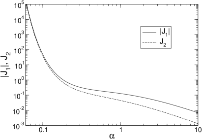
Figure 4: Constants $J_{1}(\alpha)$ and $J_{2}(\alpha)$ from Eq. (84).

Because of the angular momentum projection conservation $m_{\mathrm{A}}+m_{\mathrm{B}}=m^{\prime}_{\mathrm{A}}+m^{\prime}_{\mathrm{B}}$ the next minimal $m_{+}=2$ will be for the matrix element between the states with one of $m_{\mathrm{A}}$, $m_{\mathrm{B}}=1$, the other zero. Such atomic states (and only them) convert to molecular $\Pi$ states, which thus will have splitting $R^{7/2\alpha-2}e^{-2\alpha R}$. Arranging the four states in the following order $|m_{\mathrm{A}}m_{\mathrm{B}}\rangle=|0,1\rangle$, $|1,0\rangle$, $|0,-1\rangle$, $|-1,0\rangle$, we find that the matrix $J_{m_{\mathrm{A}}m_{\mathrm{B}}m^{\prime}_{\mathrm{A}}m^{\prime}_{\mathrm{B}}}$ is

$$J = \frac{1}{4}|C_{l}|^{4}(2l+1)^{2}l(l+1)R^{7/2\alpha-2}e^{-2\alpha R}$$ (83)

$$\times \left(\begin{array}[]{cccc}J_{2}&J_{1}&0&0\\ J_{1}&J_{2}&0&0\\ 0&0&J_{2}&J_{1}\\ 0&0&J_{1}&J_{2}\end{array}\right),$$

where

$$J_{1} = -\frac{1}{\alpha}\left(2+\frac{1}{2\alpha}\right)I(\alpha),$$

$$J_{2} = \frac{\Gamma\left(1/2\alpha\right)}{2^{3+\frac{1}{\alpha}}\alpha^{4+\frac{1}{2\alpha}}}$$ (84)

$$\int_{0}^{1}e^{\frac{y-1}{\alpha}}(1-y)^{\frac{3}{2\alpha}-1}(1+y)^{\frac{1}{2\alpha}-1}(1+y^{2})dy.$$

These constants are plotted as functions of $\alpha$ in Fig. 4.

Matrix (83) has two doubly-degenerate eigenvalues $J_{2}\pm J_{1}\equiv J_{2}\mp|J_{1}|$. Hence eight-fold degenerate two-electron state will split into four doubly-degenerate coordinate states located in the order shown in Fig. 5. The correct combination of two-electron wave functions converting into molecular terms are presented in Fig. 5 for the total projection of the orbital momentum $L=1$. The second degenerate state with $L=-1$ for each term is given by substitution of 1 with $-1$ in the two-electron wave functions.

Figure 5: Sketch of the energy level splitting of $p$-states of hydrogenic atoms under exchange interaction in diatomic molecule (in units of $\frac{1}{4}|C_{l}|^{4}(2l+1)^{2}l(l+1)R^{7/2\alpha-2}e^{-2\alpha R}$).

Note that unlike the energy level splitting of $s$-terms, the lowest energy term of the two atoms each in a $p$-state turns out to be spin-triplet while the most excited — spin-singlet.

References

• (1) K. C. Ku, S. J. Potashnik, R. F. Wang, M. J. Seong, E. Johnston-Halperin, R. C. Meyers, S. H. Chun, A. Mascarenhas, A. C. Gossard, D. D. Awschalom, P. Schiffer, N. Samarth, Appl. Phys. Lett. 82, 2302 (2003).
• (2) T. Dietl, H. Ohno and F. Matsukura, Phys. Rev. B 63, 195205 (2001).
• (3) K. Andres, R. N. Bhatt, P. Goalwin, T. M. Rice, and R. E. Walstedt, Phys. Rev. B 24, 244 (1981).
• (4) C. Herring, Rev. Mod. Phys. 34, 631 (1962).
• (5) L. P. Gor’kov and L. P. Pitaevskii, Dokl. Acad. Nauk SSSR 151, 822 (1963) [Sov. Phys. Dokl. 8, 788 (1964)].
• (6) C. Herring and M. Flicker, Phys. Rev. 134, A362 (1964).
• (7) B. M. Smirnov and M. I. Chibisov, Zh. Exp. Teor. Fiz. 48, 939 (1965) [Sov. Phys. JETP 21, 624 (1965)].
• (8) M. I. Chibisov and R. K. Janev, Phys. Rep. 166, 1 (1988).
• (9) S. Ja. Umanski and A. I. Voronin, Theor. Chim. Acta 12, 166 (1968).
• (10) E. E. Nikitin and S. Ya. Umanskii, Theory of Slow Atomic Collisions (Springer, New York, 1984).
• (11) G. Hadinger, G. Hadinger, O. Bouty, and M. Aubert-Frećon, Phys. Rev. A 50, 1927 (1994).
• (12) I. V. Ponomarev, V. V. Flambaum, A. L. Efros, Phys. Rev. B 60, 5485; ibid., 15848 (1999).
• (13) J. M. Luttinger and W. Kohn, Phys. Rev. 97, 869 (1955).
• (14) J. M. Luttinger, Phys. Rev. 102, 1030 (1956).
• (15) W. Kohn and J. M. Luttinger, Phys. Rev. 98, 915 (1955).
• (16) A. A. Abramov, V. V. Ditkin, N. V. Konyukhova, V. S. Pariiskii and V. I. Ul’yanova, U.S.S.R. Comput. Maths. Math. Phys. 20, 63 (1981).
• (17) G. Dresselhaus, Phys. Rev. 100, 580 (1955).
• (18) M.I. Dyakonov and V.I. Perel, Fiz. Tverd. Tela 13, 3581 (1971) [Sov. Phys. Solid State 13, 3023 (1972)]; Zh. Exp. Teor. Fiz. 65, 362 (1973) [Sov. Phys. JETP 38, 177 (1974)].
• (19) L. P. Gor’kov and P. L. Krotkov, Phys. Rev. B 67, 033203 (2003).
• (20) K.V.Kavokin, cond-mat/0212347 (unpublished).
• (21) A. Baldereschi and N. O. Lipari, Phys. Rev. B 8, 2697 (1973).
• (22) N. O. Lipari and A. Baldereschi, Phys. Rev. Lett. 25, 1660 (1970).
• (23) B. L. Gel’mont and M. I. D’yakonov, Fiz. Tekh. Poluprovodn. 5, 2191 (1971) [Sov. Phys. Semicond. 5, 1905 (1972)].
• (24) B. I. Shklovskii and A. L. Efros, Electronic Properties of Doped Semiconductors, Chapter 1 (Springer, N. Y., 1984).
• (25) A. V. Malyshev and I. A. Merkulov, Phys. Solid State 39, 49 (1997).