Improved self-absorption correction for fluorescence measurements
of extended x-ray absorption fine-structure

Abstract

Extended x-ray absorption fine-structure (EXAFS) data collected in the fluorescence mode are susceptible to an apparent amplitude reduction due to the self-absorption of the fluorescing photon by the sample before it reaches a detector. Previous treatments have made the simplifying assumption that the effect of the EXAFS on the correction term is negligible, and that the samples are in the thick limit. We present a nearly exact treatment that can be applied for any sample thickness or concentration, and retains the EXAFS oscillations in the correction term.

Under ideal circumstances, such as a very dilute sample, the photoelectric part of the x-ray absorption coefficient, $\mu$, is proportional to the number of fluorescence photons escaping the sample. However, in extended x-ray absorption fine-structure spectroscopy (EXAFS), the mean absorption depth changes with the energy of the incident photon, $E$, which changes the probability that the fluorescence photon will be reabsorbed by the sample. This self-absorption causes a reduction in the measured EXAFS oscillations, $\chi_{exp}$, from the true $\chi$, and hence needs to be included in any subsequent analysis.

Previous treatments Goulon et al. (1982); Tan et al. (1989); Tröger et al. (1992) to correct for the self-absorption effect account for the change in depth due to the absorption edge and due to the smooth decrease in $\mu$ that follows, for instance, a Victoreen formula, and have been shown to be quite effective in certain limits. These treatments typically make two important assumptions. First, the so-called “thick limit” is used to eliminate the dependence on the actual sample thickness, limiting the applicability to thick, concentrated samples, such as single crystals. One exception is the work of Tan, Budnick and Heald Tan et al. (1989), which makes a number of other assumptions to estimate the correction to the amplitude reduction factor, $S_{0}^{2}$, and to the Debye-Waller factors, $\sigma^{2}$’s, rather than correcting the data in a model-independent way. A second assumption is that, in order to make the correction factor analytical, at one point in the calculation, the true absorption coefficients for the absorbing species and the whole sample are replaced with their average values; in other words, the modulating effect of $\chi$ on the correction factor is taken as very small. Below, we present a treatment that, with only one assumption that is nearly exact for all cases we have measured, corrects fluorescence EXAFS data directly in $k$-space for any concentration or thickness. This correction is demonstrated for a copper foil that is about one absorption-length thick, and is therefore not in the thick limit.

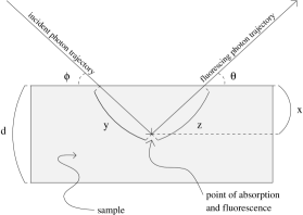
Figure 1: Geometry used in calculating self-absorption correction in EXAFS.

.

Figure 1 shows the geometry used in this calculation. The fluorescence yield at the point of absorption is proportional to the x-ray intensity $I$ at that point and the fluorescence efficiency. The intensity $I$ at a depth $y$ is

$$I=I_{0}e^{-\mu(E)y}.$$

The fluorescence photon then has to escape. The fluorescence flux from this point in the sample is then

$$I_{f}=I_{0}e^{-\mu(E)y}e^{-\mu(E_{f})z}\epsilon_{a}(E)\mu_{a}(E),$$

where $\mu_{a}(E)$ is the absorption due to the absorbing atom, $\mu(E)$ is the total absorption, $\epsilon_{a}(E)$ is the fluorescence efficiency per unit solid angle, $E$ is the incident beam energy, $E_{f}$ is the energy of the fluorescing photon, and we’re assuming that all the measured fluorescence is coming from the desired process (eg. Cu $K_{\alpha}$, any other counts can be subtracted off). This equation is only true at a particular $y$ and $z$, so we must integrate

$$dI_{f}=I_{0}\epsilon_{a}\mu_{a}e^{-(\mu_{T}y+\mu_{f}z)}dy.$$

Here the energy dependences are implicit and we’ve used $\mu_{T}=\mu(E)$ and $\mu_{f}=\mu(E_{f})$. The variables $z$ and $y$ are dependent via $y\sin\phi=z\sin\theta=x$. Changing variables, we obtain

$$dI_{f}=I_{0}\epsilon_{a}\mu_{a}\frac{1}{\sin\phi}e^{-(\frac{\mu_{T}}{\sin\phi}+\frac{\mu_{f}}{\sin\theta})x}dx$$

$$I_{f} = I_{0}\epsilon_{a}\mu_{a}\frac{1}{\sin\phi}\int_{0}^{d}e^{-(\frac{\mu_{T}}{\sin\phi}+\frac{\mu_{f}}{\sin\theta})x}dx$$

$$I_{f} = \frac{I_{0}\epsilon_{a}\mu_{a}}{\mu_{T}+g\mu_{f}}\left[1-e^{-(\frac{\mu_{T}}{\sin\phi}+\frac{\mu_{f}}{\sin\theta})d}\right],$$ (1)

where $g\equiv\frac{\sin\phi}{\sin\theta}$. Eq. 1 describes the fluorescence in the direction given by $\theta$. At this point one should integrate over the detector’s solid angle. Ignoring this integral can affect the final obtained correction Brewe et al. (1994), especially for glancing-emergent angle experiments. However, for detector geometries where $\phi+\theta=90^{\circ}$, we find the maximum error in $g$ is on the order of $\sim 1-2\%$ even for $\Delta\theta\approx 5^{\circ}$ at $\theta=80^{\circ}$. For more severe geometries, the solid angle should be considered, but for the following, we ignore this correction.

In EXAFS measurements, we want

$$\chi=\frac{\mu_{a}-\bar{\mu_{a}}}{\bar{\mu_{a}}},$$

but what we actually obtain experimentally is

$$\chi_{exp}=\frac{I_{f}-\bar{I_{f}}}{\bar{I_{f}}},$$

where $\bar{I_{f}}$ is the spline function fit to the data to simulate the “embedded atom” background fluorescence (roughly $I_{f}$ without the EXAFS oscillations). Now make the following substitutions:

$$\mu_{T} = \bar{\mu_{T}}+\chi\bar{\mu_{a}}$$

$$\mu_{a} = (\chi+1)\bar{\mu_{a}}$$

$$\mu_{T}-\bar{\mu_{T}} = \mu_{a}-\bar{\mu_{a}}.$$

These equations and Eq. 1 are then plugged into $\chi_{exp}$:

$$1+\chi_{exp}=\frac{\mu_{a}(\bar{\mu_{T}}+g\mu_{f})[1-e^{-(\frac{\mu_{T}}{\sin\phi}+\frac{\mu_{f}}{\sin\theta})d}]}{\bar{\mu_{a}}(\mu_{T}+g\mu_{f})[1-e^{-(\frac{\bar{\mu_{T}}}{\sin\phi}+\frac{\mu_{f}}{\sin\theta})d}]}.$$

Dividing by $1+\chi$ and defining $\alpha\equiv\bar{\mu_{T}}+g\mu_{f}$, we get:

$$\frac{1+\chi_{exp}}{1+\chi}=\frac{[1-e^{-(\bar{\mu_{T}}+\chi\bar{\mu_{a}}+g\mu_{f})\frac{d}{\sin\phi}}]\alpha}{(\alpha+\chi\bar{\mu_{a}})[1-e^{-\frac{\alpha d}{\sin\phi}}]}.$$

Now $\chi_{exp}$ can be written in terms of the actual $\chi$:

$$\chi_{exp}=\left[\frac{1-e^{-(\alpha+\chi\bar{\mu_{a}})\frac{d}{\sin\phi}}}{1-e^{-\frac{\alpha d}{\sin\phi}}}\right]\left[\frac{\alpha(\chi+1)}{\alpha+\chi\bar{\mu_{a}}}\right]-1.$$ (2)

At this point in the calculation, the relation between $\chi$ and $\chi_{exp}$ is exact. However, we need $\chi$ in terms of $\chi_{exp}$, and Eq. 2 is for $\chi_{exp}$ in terms of $\chi$. In order to invert Eq. 2, we make a simple approximation. Assuming that

$$\frac{\chi\bar{\mu_{a}}d}{\sin\phi}<<1$$

we can say

$$1-e^{-(\alpha+\chi\bar{\mu_{a}})\frac{d}{\sin\phi}}\sim 1-e^{-\frac{\alpha d}{\sin\phi}}(1-\frac{\chi\bar{\mu_{a}}d}{\sin\phi}).$$ (3)

This approximation gets worse with large $\chi$ and $\bar{\mu_{a}}$. It also has a maximum for both $\phi$ and $d$, because of the $e^{-\frac{\alpha d}{\sin\phi}}$ term. Plugging in some typical numbers from the Cu $K$-edge of YBa₂Cu₃O₇ ($\phi=10^{\circ}$, $\bar{\mu_{T}}=01.32\mu$m${}^{-1},\mu_{F}=1.10\mu$m${}^{-1},\bar{\mu_{a}}=1.0\mu$m^-1 and $\chi=0.5$) the maximum error is $\sim 2.7\%$ at a thickness of $\sim 1.9\mu$m. Such a high value of $\chi$ does not actually occur in YBCO. Indeed, such a high $\chi$ is very rare. In any case, various combinations of the above parameters can conspire to produce errors above 1%, so the approximation should be monitored when making the corrections outlined below.

With the above approximation, and defining the following quantities:

$$\beta = \frac{\bar{\mu_{a}}d\alpha}{\sin\phi}e^{-\frac{\alpha d}{\sin\phi}}$$

$$\gamma = 1-e^{-\frac{\alpha d}{\sin\phi}},$$

Eq. 2 is reduced to a quadratic equation in $\chi$ and we can finally write the full correction formula:

$$\chi=\frac{-[\gamma(\alpha-\bar{\mu_{a}}(\chi_{exp}+1))+\beta]+\sqrt{[\gamma(\alpha-\bar{\mu_{a}}(\chi_{exp}+1))+\beta]^{2}+4\alpha\beta\gamma\chi_{exp}}}{2\beta},$$ (4)

where the sign of the square root was determined by taking the thick or thin limits. In the thick limit ($d\rightarrow\infty$), Eq. 4 gives:

$$\chi=\frac{\chi_{exp}}{1-\frac{\bar{\mu_{a}}}{\alpha}\chi_{exp}-\frac{\bar{\mu_{a}}}{\alpha}},$$

which is the same as calculated in Ref. Tröger et al. (1992) without the $\chi_{exp}$ term in the denominator. In the thin limit, it can be shown that Eq. 4 reduces to $\chi=\chi_{exp}$, as expected.

Figure 2: Correction term $\chi/\chi_{exp}$ given by Eq. 4 for Cu $K$-edge absorption data from a 4.6 $\mu$m-thick copper foil at $\phi=49.4^{\circ}$.

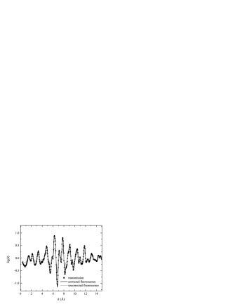
Figure 3: Corrected EXAFS data in $k$-space for the copper foil data, compared to transmission data and uncorrected fluorescence data. Note that the corrected data are difficult to discern on top of the transmission data.

We performed an experiment on a copper foil to demonstrate the correction. Cu $K$-edge data were collected both in the transmission mode and in the fluorescence mode using a 32-element Canberra germanium detector on beam line 11-2 at the Stanford Synchrotron Radiation Laboratory (SSRL). The transmission data were checked for pinhole effects (found to be negligible) and the fluorescence data were corrected for dead time. The sample thickness was estimated to be 4.6 $\mu$m from the absorption step at the edge, and was oriented such that $\phi=49.4\pm 0.5^{\circ}$. The thickness is about 25% of the estimated thick-limit thickness. The data were reduced to $k$-space using the RSXAP analysis program REDUCE Hayes and Boyce (1982); Li et al. (1995); RSX , which incorporates these corrections. Figure 2 shows the correction factor ($\chi/\chi_{exp}$) for these data. The error in the approximation in Eq. 3 exceeds 1% only below $\sim 1$Å^-1. The total correction in the thick limit is much larger (about 3 times the displayed correction). As shown in Fig. 3, the corrected fluorescence data in $k$-space are remarkably similar to the transmission data, despite the large magnitude of the correction.

Although only a copper foil is reported as an example, we have successfully applied this correction to a wide range of oxides and intermetallics, including single crystals and thin films Booth et al. (1996); Ren et al. (1998); Cao et al. (2000); Mannella et al. (2003); Booth et al. . The ability to correct for intermediate film thicknesses is, in fact, crucial for studying films thinner than $\sim 20\mu$m thick.

In summary, we have provided an improved self-absorption correction for EXAFS data that operates at any sample thickness or concentration. Our example of a pure copper foil demonstrates both the accuracy of the correction and that, for concentrated samples, the correction can be surprisingly large. Moreover, for well-ordered materials, $\chi$ can have a surprisingly large effect.