Electron transfer rates for asymmetric reactions

Abstract

We use a numerically exact real-time path integral Monte Carlo scheme to compute electron transfer dynamics between two redox sites within a spin-boson approach. The case of asymmetric reactions is studied in detail in the least understood crossover region between nonadiabatic and adiabatic electron transfer. At intermediate-to-high temperature, we find good agreement with standard Marcus theory, provided dynamical recrossing effects are captured. The agreement with our data is practically perfect when temperature renormalization is allowed. At low temperature we find peculiar electron transfer kinetics in strongly asymmetric systems, characterized by rapid transient dynamics and backflow to the donor.

1 Introduction

This paper presents results of computer simulations for simple asymmetric electron transfer (ET) reactions in polar solvents. Such reactions are encountered in a large variety of different systems, e.g. charge transfer in semiconductors, chemical reactions, or the primary step in bacterial photosynthesis [1, 2, 3, 4, 5, 6]. Our theoretical study of such processes is based on the spin-boson (SB) model (dissipative two-level system) [7]. This model provides an accurate description of many ET reactions involving condensed-phase environments [4], if a suitable spectral density $J(\omega)$ can be determined for these “bath” modes. For a detailed discussion of restrictions for the SB description of ET reactions, including an (almost) exhaustive list of references to work done in that context, we refer to our previous work [8] for symmetric ET reactions. In the present paper, primary focus is laid on the asymmetric case. Within the SB model, the localized sites representing the donor and the acceptor are described in terms of an effective, quantum mechanical “spin” variable. The two-level system (TLS) is characterized by a tunnel splitting $\hbar\Delta$, which is twice the usual electronic coupling between the redox sites, and by the asymmetry $\hbar\epsilon$ giving the energy difference between the two localized states. The frequency-resolved coupling strength of the electron to the surrounding solvent modes is then described by the spectral density, where one mimics the environment by an infinite set of effective harmonic oscillators. The spectral density for a given ET reaction can in principle be computed from classical molecular dynamics simulations [4], but in many cases it turns out to be appropriate to consider the special class of Ohmic spectral densities [5, 7],

$$J(\omega)=2\pi\alpha\omega\,\e^{-\omega/\omega_{c}},$$ (1)

with dimensionless damping strength $\alpha$ and a cutoff frequency $\omega_{c}$. On general grounds, the linear low-frequency behavior of $J(\omega)$ is expected in basically all condensed-phase ET reactions [4, 5], and the frequency $\omega_{c}$ then corresponds to some dominant bath mode. To make contact with common notation, we shall use the reorganization energy $\hbar\Lambda$ [1] instead of $\alpha$, where $\Lambda=2\alpha\omega_{c}$. While our method below is able to treat arbitrary spectral densities, for clarity we will only present data using Eq. (1). Note that for common ET reactions, one has large damping parameters $\alpha$, and therefore one is always in the incoherent regime with respect to the electronic degree of freedom. Coherence is nevertheless possible with respect to the bath degrees of freedom, in particular when fast bath modes are absent or particular initial preparations are selected [9, 10]. We mention in passing that due to the strong damping, weak-coupling Redfield-type approaches [11] are not suitable for a description of condensed-phase ET processes.

For very large $\omega_{c}/\Delta$ and sufficiently low temperatures, the scaling limit of the SB model is reached, where powerful analytical methods are available [5, 7]. Unfortunately, the scaling regime is of little relevance to ET reactions, but in certain parameter regions, progress is nevertheless possible. A famous and very successful description of ET reactions concerns the high-temperature limit, where the bath behaves classically, leading to Marcus theory [1]. Indeed, it can be shown that the classical limit of the SB model directly gives Marcus theory [12, 13]. Another example is given by the golden rule formula for the nonadiabatic ET rate [14, 15], which is accurate for arbitrary temperature as long as $\Delta/\omega_{c}\ll 1$. In the opposite adiabatic limit of a very slow (classical) bath, analytical progress is also possible [16]. A particular focus of our study lies on the crossover regime between adiabatic and nonadiabatic ET, which represents the most difficult and least understood regime from a theory point of view, in particular at low temperatures.

In our previous work [8], exactly this regime was studied for symmetric systems. Applying the path-integral Monte Carlo (PIMC) scheme of Ref. [8] to $\epsilon\neq 0$, we are able to directly monitor the ET dynamics without any approximation. This should be contrasted to alternative numerical routes to this problem. For instance, in mixed quantum/(semi)classical simulations for the SB model [17, 18, 19, 20, 21], it is hard to justify some of the approximations, and hence the accuracy of the results has to be checked case by case. Similar arguments apply to basis set calculations [22], and to memory-equation approaches [23, 24]. Other methods are known to be accurate, but only in either the scaling regime or the weak-coupling regime [25, 26, 27, 28]. We conclude that the PIMC method represents an excellent computer simulation method for treating the crossover regime mentioned above. PIMC is free from approximations, but has to deal with the well known dynamical sign problem, because a calculation of ET rates requires dynamical information incorporating interfering real-time trajectories. Some workers have attempted to use analytical continuation of imaginary-time PIMC data [29, 30, 31], but this process is mathematically ill-defined and troublesome to carry out. Here we instead directly proceed in real time, where reliable error estimates can be obtained and true nonequilibrium preparations can be investigated [8, 32]. The outline of the paper is as follows. In Sec. 2, we summarize the model and the simulation technique. Results for asymmetric ET reactions are presented in Sec. 3. We close with a concluding discussion in Sec. 4.

2 Spin-boson description of ET reactions

The spin-boson model [5, 7] is defined by a coupled system-bath Hamiltonian $H=H_{0}+H_{I}+H_{B}$. The “spin” corresponding to the TLS is parametrized by Pauli matrices $\sigma_{i}$, where the $|+\rangle$ ($|-\rangle$) eigenstate of $\sigma_{z}$ refers to the donor (acceptor). In the absence of the solvent, this leads to

$$H_{0}=-{\hbar\Delta\over 2}\sigma_{x}+{\hbar\epsilon\over 2}\sigma_{z}.$$ (2)

The environmental modes are modeled by an infinite collection of harmonic oscillators, $H_{B}$, which bilinearly couple to the position of the electron ($H_{I}$). The solvent-TLS coupling is completely encoded in a spectral density $J(\omega)$, which effectively becomes a continuous function of $\omega$ for condensed-phase environments, and determines all bath correlation functions that are relevant for ET dynamics. Here we take the Ohmic form (1) as a prototype spectral density. The bath autocorrelation function for complex time $z=t-\mathrm{i}\tau$ is (with $\beta=1/k_{\rm B}T$)

$$L(z)=\int_{0}^{\infty}\frac{\d\omega}{\pi}J(\omega){\cosh[\omega(\hbar\beta/2-\mathrm{i}z)]\over\sinh(\hbar\beta\omega/2)}.$$ (3)

In the classical limit, the reorganization energy $\hbar\Lambda$, which is an integral quantity describing the overall coupling strength, is the only important bath quantity. Details of the frequency dependence of $J(\omega)$ become crucial only at low temperatures.

Here we study two dynamical properties characterizing ET kinetics. First,

$$P(t)=\langle\sigma_{z}(t)\rangle=\langle\e^{\mathrm{i}Ht/\hbar}\sigma_{z}\e^{-\mathrm{i}Ht/\hbar}\rangle$$ (4)

gives the difference in occupation probabilities of the donor and the acceptor state, with the electron initially fixed on the donor. This quantity then directly probes ET dynamics after a nonequilibrium initial preparation, e.g. following photoexcitation of an electron into the donor state. Second, the correlation function

$$C(t)=\langle\sigma_{z}(0)\sigma_{z}(t)\rangle_{\beta}=Z^{-1}{\rm tr}\left\{\e^{-\beta H}\sigma_{z}\e^{\mathrm{i}Ht/\hbar}\sigma_{z}\e^{-\mathrm{i}Ht/\hbar}\right\}$$ (5)

with $Z={\rm tr}\{\exp(-\beta H)\}$ probes the dynamics under an equilibrium preparation. At high temperatures, preparation effects are not expected to dramatically affect the ET dynamics, and therefore a well-defined thermal rate $k_{\rm th}$ should exist [33, 34]. This rate then supposedly governs the exponential relaxation of both $P(t)$ and $C(t)$ on a timescale of the order of $\tau_{\rm relax}\approx k_{\rm th}^{-1}$. In principle, at low temperatures, this assertion can be violated, and then the relevant quantity of interest depends on the experimental setup under consideration.

In case a unique rate constant exists, it is composed of the forward rate $k_{\mathrm{f}}$ and the backward rate $k_{\mathrm{b}}$, referring to directed transfers between the donor and acceptor states according to

$$dP_{+}=(-k_{f}P_{+}+k_{b}P_{-})dt\;,\quad dP_{-}=(-k_{b}P_{-}+k_{f}P_{+})dt$$

for times beyond some transient timescale, $t>\tau_{\rm trans}\approx 1/\omega_{\mathrm{c}}$. Under such a rate process, ET dynamics obeys

$$P(t>\tau_{\rm trans})=P_{\rm trans}\exp(-k_{\rm th}t)+P_{\infty},$$ (6)

where $P_{\infty}=\langle\sigma_{z}\rangle_{\beta}$ denotes the electronic equilibrium population,

$$P_{\rm trans}=[P(\tau_{\rm trans})-P_{\infty}]\exp(k_{\rm th}\tau_{\rm trans}),$$

and $k_{\mathrm{th}}$ is the total transfer rate $k_{\mathrm{f}}+k_{\mathrm{b}}$. Accordingly, $P(t)$ follows a simple exponential decay for times $t>\tau_{\rm trans}$.

Another way to obtain the thermal transfer rate $k_{\rm th}$ is via a time-dependent equilibrium rate function [33, 34]. Assuming that $k_{\mathrm{f}}$ and $k_{\mathrm{b}}$ are connected via a standard detailed balance relation,

$$k_{\mathrm{b}}=k_{\mathrm{f}}\exp(-\hbar\beta\epsilon)\;,$$ (7)

for the SB model this function reads [8]

$$k(t)={1+\cosh(\hbar\beta\epsilon)\over\hbar\beta}{\rm Im}C(t),$$ (8)

where we exploited that Eq. (7) corresponds to the assumption of a Boltzmann distribution for the equilibrium occupation probabilities, $P_{\infty}=-\tanh(\hbar\beta\epsilon/2)$. This is expected to always hold under the strong damping conditions characteristic for ET reactions. Indeed, our numerical results below verify this assumption to high precision.

According to the reasoning in Ref. [33], $k_{\rm th}$ is then obtained as the plateau value of $k(t)$ if such a plateau exists. However, a careful re-examination of the argument in Ref. [33], see also Ref. [35], reveals that this procedure is just the limiting case of a more general situation, where $k(t)$ decays exponentially according to

$$k(t>\tau_{\rm trans})=k_{\rm th}e^{-k_{\rm th}t}.$$ (9)

Therefore, even if Eq. (8) exhibits no clear plateau, a reaction rate can still be extracted if the “exponential fit” to Eq. (9) is possible. A concrete example is shown in Fig. 1, where the PIMC data for $P(t)$ and $k(t)$ are both consistent with the same thermal rate constant $k_{\rm th}=0.097\Delta$. The exponential fit to Eq. (9) is generally more accurate than extracting $k_{\rm th}$ directly from $P(t)$, where transient decays for $t<\tau_{\rm trans}$ complicate the analysis. The latter approach was taken in Ref. [8] whenever no plateau was found for $k(t)$, but then the rates could have been obtained to better precision using the exponential fitting procedure for $k(t)$. We mention in passing that regarding Fig. 7 of Ref. [8], ET rates for $T\geq 2\hbar\Delta/k_{\rm B}$ indeed closely follow the classical Marcus rate, see Eq. (10) below, if one takes a renormalized temperature $T^{\prime}=0.87T$ ($0.78T$) for $\Lambda/\Delta=10$ and $\Delta/\omega_{\mathrm{c}}=1$ ($\Delta/\omega_{\mathrm{c}}=2$). Obviously, fits to Eq. (9) can fail, in particular when (vibrational) coherence survives, or when $\tau_{\rm trans}$ and $\tau_{\rm relax}$ are not sufficiently well separated. Such problems will then indicate the invalidity of a simple rate picture in these cases.

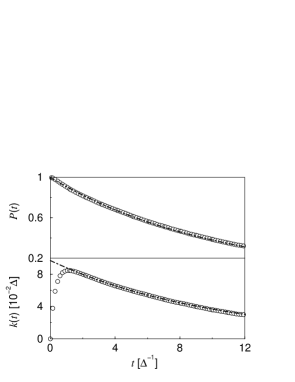
Figure 1: ET dynamics for $\Lambda/\Delta=15$, $\epsilon=0$, $\Delta/\omega_{\mathrm{c}}=0.067$, and $T=\hbar\Delta/k_{\rm B}$. Shown are PIMC data for $P(t)$ (top) and $k(t)$ (bottom). Dashed curves are $\exp(-k_{\rm th}t)$ (top) and $k_{\rm th}\exp(-k_{\rm th}t)$ (bottom), with $k_{\rm th}=0.097\Delta$. Error bars (one standard deviation) are smaller than symbol size.

Before describing the PIMC method employed here, we briefly review classical Marcus theory [1]. Writing the thermal transfer rate in terms of the forward rate, $k^{\rm cl}=k^{\rm cl}_{\rm f}(1+\e^{-\hbar\epsilon/k_{\rm B}T})$, Marcus theory predicts

$$k^{\rm cl}_{\rm f}=\frac{\Delta^{2}}{4+\pi\Delta^{2}/(\Lambda\omega_{\rm r})}\sqrt{{\pi\hbar\over\Lambda k_{\rm B}T}}\,\e^{-F^{\ast}(\epsilon)/k_{\rm B}T},$$ (10)

with the activation free energy barrier (Marcus parabola)

$$F^{\ast}(\epsilon)=\hbar(\epsilon-\Lambda)^{2}/4\Lambda,$$ (11)

and a solvent frequency scale $\omega_{\rm r}$. The $\omega_{\rm r}$ dependent prefactor in Eq. (10) was introduced by Zusman [2] to account for recrossing events. The scale $\omega_{\rm r}$ seems to follow a power law at low temperatures [8], but in the true classical (high-temperature) regime, it is given by $\omega_{\rm r}=\omega_{\mathrm{c}}/2$ [8, 12]. Marcus theory (supplemented by dynamical recrossing effects) yields a classical rate constant covering the full crossover from nonadiabatic to adiabatic ET. One of its most striking features is a non-monotonic behavior of the forward rate as a function of asymmetry $\epsilon$. According to Eq. (11), $k^{\rm cl}_{\rm f}$ exhibits its single maximum in the activationless case $\epsilon=\Lambda$, but decreases again in the inverted regime $\epsilon>\Lambda$. While experiments qualitatively support this picture [36], quantum effects (nuclear tunneling) not captured by Marcus theory should play a major role in the inverted regime [1]. Such effects are of course included by the PIMC simulations below.

Next we briefly describe our computational technique used to calculate ET rate constants (if they exist) under a spin-boson description. A detailed exposition of our method can be found in Ref. [8], and here we only sketch it to keep the paper self-consistent. After tracing out the Gaussian bath degrees of freedom in Eqs. (4) and (5), one arrives at path-integral expressions for the dynamical quantities of interest, where only the TLS degree of freedom is kept explicitly. For instance,

$$C(t)=Z^{-1}\int\!{\mathcal{D}}\sigma\;\sigma(0)\sigma(t)\exp\left\{{\mathrm{i}\over\hbar}S_{0}[\sigma]-\Phi[\sigma]\right\},$$ (12)

where the path integration runs over paths $\sigma(z)$ for the discrete spin variable $\sigma=\pm 1$ corresponding to the eigenvalues of $\sigma_{z}$, with the complex time $z$ following the Kadanoff-Baym contour $\gamma=\{z:0\rightarrow t\rightarrow 0\rightarrow-\mathrm{i}\hbar\beta\}$. $S_{0}[\sigma]$ denotes the free TLS action, while the effective action due to the traced-out bath is captured by the influence functional [5]

$$\Phi[\sigma]={1\over 4}\int_{\gamma}\d z\int_{z^{\prime}<z}\d z^{\prime}\sigma(z)L(z-z^{\prime})\sigma(z^{\prime}),$$ (13)

with integrations ordered along the contour $\gamma$. For a numerical evaluation, time is discretized, and, moreover, the real-time spins $\sigma(t^{\prime})$ and $\sigma^{\prime}(t^{\prime})$ on the forward and backward branch of the Kadanoff-Baym contour $\gamma$ are combined to form quantum fluctuations ($\sigma-\sigma^{\prime}$) and quasiclassical variables ($\sigma+\sigma^{\prime}$) which are sampled stochastically in the course of the PIMC simulation. Technical details about our implementation of this program can be found in Ref. [8].

While similar expressions can be derived for the occupation probability, $P(t)$ can also be obtained from the same MC trajectory as $C(t)$ (and therefore $k(t)$) by including a correction factor that accommodates the changes in the corresponding MC weight [8]. In principle, this allows to simultaneously compute $k(t)$ and $P(t)$ without significant increase in computing time. However, for a strongly biased system, $\epsilon/\Lambda\gg 1$, this approach has a rather poor performance since the respective MC weights refer to almost orthogonal initial electronic states. It would then be necessary to run separate simulations to extract $P(t)$ and $k(t)$. More serious complications arise from the fact that $k(t)$ in Eq. (8) is composed of two competing contributions, namely $[1+\cosh(\hbar\beta\epsilon)]$ and ${\rm Im}C(t)/\hbar\beta$. Since the former increases exponentially with $|\epsilon|$, the latter should be very tiny in order to give a finite result. Unfortunately, our simulations show that the stochastic PIMC error in ${\rm Im}C(t)$ is rather insensitive to a change of parameters, as long as the time scale of the simulation is kept fixed. Hence relative errors become arbitrarily large as ${\rm Im}C(t)\to 0$, which renders data for $k_{\rm th}$ numerically unstable. Since the relevant parameter is $|\hbar\beta\epsilon|$, extraction of $k_{\rm th}$ from $k(t)$ fails already at rather small $|\epsilon|$ for low temperature. These numerical problems are unrelated to the dynamical sign problem, which did not impose serious limitations in the parameter regime investigated here. Therefore, there was no need to employ the powerful but complicated “multilevel blocking” algorithm [8] to relieve the sign problem.

3 Numerical results for asymmetric ET

\psfrag{E}{$\epsilon$}\includegraphics[height=213.39566pt,draft=false]{sigma_beta.eps}

Figure 2: Equilibrium expectation value $\langle\sigma_{z}\rangle_{\beta}$ as a function of $\epsilon$ for $T=\hbar\Delta/k_{\rm B}$ (circles) and $T=10\hbar\Delta/k_{\rm B}$ (diamonds). The dashed and dotted lines refer to $-\tanh(\hbar\beta\epsilon/2)$. Solvent parameters are $\Delta/\omega_{\mathrm{c}}=1$ and $\Lambda=10\Delta$.

Being mainly interested in the effect of the asymmetry $\epsilon$ on the ET dynamics, we have calculated both the occupation probability $P(t)$ and the time-dependent rate function $k(t)$ for various values of $\epsilon$ at a high and a low temperature. Specifically, we consider $T=10\hbar\Delta/k_{\rm B}$ and $T=\hbar\Delta/k_{\rm B}$, and take bath parameters where Marcus theory has been shown to be accurate in the symmetric case [8], namely $\Delta/\omega_{\mathrm{c}}=1$ and $\Lambda=10\Delta$. This parameter choice represents the most interesting crossover region between nonadiabatic and adiabatic ET.

For these temperatures, from closer inspection of Eq. (10), the rate $k_{\rm th}(\epsilon)$ is expected to exhibit a single maximum at $\epsilon=0$ for the higher temperature, but two symmetric maxima at $\epsilon=\pm\epsilon_{\rm max}$ with $\epsilon_{\rm max}<\Lambda$ for the lower one. From Eq. (10), it is easy to see that $\epsilon_{\rm max}$ is a solution of the equation

$$(1-\epsilon/\Lambda)[1+\exp(\hbar\beta\epsilon)]=2.$$

Furthermore, due to Eq. (7), the thermal transfer rate is a symmetric function of $\epsilon$. Quantum corrections to the classical rate (10) are then of primary interest to us, in particular in the inverted regime, $|\epsilon|>\Lambda$, for both signs of the asymmetry. Before turning to the thermal transfer rate, we show the equilibrium expectation value of $\sigma_{z}$ as a function of $\epsilon$, see Fig. 2. For the parameters investigated, we find to high precision $\langle\sigma_{z}\rangle_{\beta}=-\tanh(\hbar\beta\epsilon/2)$, as has already been mentioned above.

\psfrag{E}{$\epsilon$}\includegraphics[height=213.39566pt,draft=false]{asymmetric_high_T.eps}

\psfrag{E}{$\epsilon$}\includegraphics[height=213.39566pt,draft=false]{asymmetric_low_T.eps}

Figure 3: $k_{\rm th}(\epsilon)$ for $T=10\hbar\Delta/k_{\rm B}$ (top) and $T=\hbar\Delta/k_{\rm B}$ (bottom). The dotted (dashed) curve refers to Eq. (10) without (with) a renormalization of the temperature, $T^{\prime}=0.87T$. The larger error bars for $T=\hbar\Delta/k_{\rm B}$ and $\epsilon/\Lambda\leq-0.8$ are caused by rate extraction from $P(t)$ rather than $k(t)$.

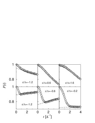
Figure 4: $P(t)$ for $T=10\hbar\Delta/k_{\rm B}$ (top) and $T=\hbar\Delta/k_{\rm B}$ (bottom). The dot-dashed curves denote fits to Eq. (6) with $k_{\rm th}$ as in Fig. 3 and (top left to top right) $P_{\rm trans}=0.41$, $1.29$, $1.72$, and (bottom left to bottom right) $-0.11,-0.24,-0.04$, respectively. For the sake of clarity, only part of the data is shown.

Starting with the high temperature $T=10\hbar\Delta/k_{\rm B}$, we then calculated the ET dynamics for $|\epsilon|/\Lambda\leq 1.8$ while keeping all other parameters fixed. Then the difficulties mentioned above did not pose serious limitations. The corresponding data for $k_{\rm th}$, which always follow from exponential fits to $k(t)$, are displayed in Fig. 3. Similar to the crossover regime for the symmetric system [8], the classical rate (10) again nicely reproduces the exact results. Our PIMC data slightly exceed the classical prediction, especially for small $|\epsilon|$. However, these deviations can be astonishingly well compensated for by the above-mentioned renormalization of the temperature. While we do not have a good theoretical argument for the validity of the temperature renormalization, we wish to stress that a renormalization of the reorganization energy and/or the activation energy is less apt to fit our data over the full asymmetry range, and moreover, completely fails to capture the mentioned deviations in the symmetric case. Notably, in the high-temperature regime, no significant trace of nuclear tunneling could be observed in the inverted regime. Outside the transient motion, ET dynamics exhibits the exponential decay (6), with slower (faster) decay than during the transient stage for $\epsilon\leq 0$ ($\epsilon>0$), see Fig. 4.

For the lower temperature $T=\hbar\Delta/k_{\rm B}$, the numerical limitations discussed above became quite severe. Extraction of the transfer rate from $k(t)$ could only be achieved for $|\epsilon|/\Lambda\leq 0.6$. Nevertheless, for $\epsilon<0$, $k_{\rm th}$ could still be obtained from $P(t)$, although with poorer accuracy since two fit parameters ($k_{\rm th}$ and $P_{\rm trans}$) are required. This extends the range of our data to $-1.4\leq\epsilon/\Lambda\leq 0.6$, and hence includes one of the rate maxima. Again the classical rate yields a remarkably accurate prediction for $k_{\rm th}$, see Fig. 3, while the temperature renormalization is seen to be limited to the high-temperature regime [8]. One might therefore be tempted to conclude that there are no significant quantum effects even at low temperatures. However, for $\epsilon/\Lambda<-0.2$, the ET dynamics shows a qualitatively different behavior. Due to the strong equilibrium localization of the electron to the donor state, the fast low-temperature initial transient kinetics is able to carry $P(\tau_{\rm trans})$ to a value below $P_{\infty}$, causing a subsequent increase of $P(t)$ towards $P_{\infty}$, see Fig 4. Nevertheless, the subsequent time evolution is still correctly captured by Eq. (6), albeit the exponentially decaying excess population with respect to its equilibrium value is now negative. This effect nicely illustrates that even outside the transient kinetics, only calculating the transfer rate is sometimes not sufficient to fully characterize the ET dynamics.

4 Discussion

Using the SB model as a description for ET processes, we have calculated the thermal transfer rate $k_{\rm th}$ for a bath setup in the crossover regime, where Marcus theory is known to provide a valid description for the symmetric electronic system. Focusing on the influence of the energy bias $\epsilon$ between the redox states, we investigated the electronic dynamics for two different temperatures, $T=\hbar\Delta/k_{\rm B}$ and $T=10\hbar\Delta/k_{\rm B}$ and various values of $\epsilon$ up to the inverted regime using real-time PIMC simulations. We extended our previous approach to extract the thermal transfer rate from the time-dependent function $k(t)$, see Eq. (8), which yields a powerful tool both to obtain $k_{\rm th}$ and to decide whether a rate description is appropriate in the first place. In the absence of electronic or vibrational coherence, this rate also describes the exponential decay of the electronic population $P(t)$, provided the timescales for transient dynamics $\tau_{\rm trans}$ and thermal relaxation $\tau_{\rm relax}$ are sufficiently well separated.

Our results for the asymmetric electronic system support the rate picture at all values of the electronic bias investigated, which extend well into the inverted regime. This also applies for the cases where the transient motion shifts the electronic population $P(t)$ below its equilibrium value, i.e. at $\epsilon<0$ and sufficiently low temperatures, where it is the subsequent deviation of $P(t)$ from this equilibrium value which decays exponentially. Furthermore, the validity of the classical rate (10) was tested as a function of the asymmetry. Deviations from the classical rate expression indicating contributions from nuclear tunneling were largely absent, suggesting that they should only play a major role at either considerably lower temperatures than $T=\hbar\Delta/k_{\rm B}$, or for very large asymmetry $|\epsilon|/\Lambda$. However, we could observe an overall enhancement of the rate which can be nicely captured by evaluating the classical rate for a renormalized temperature $T^{\prime}<T$. This phenomenon was also confirmed for the symmetric system, seems to be confined to the high-temperature regime, and becomes more pronounced towards the adiabatic limit. Furthermore, at low temperatures we found a rapid transient dynamics, followed by a backflow to the donor. This effect shows that a naive rate picture breaks down in the low-temperature regime, although the timescale for relaxation is still well predicted by the classical prediction. These findings illustrate that despite the good accuracy of classical Marcus theory, which is confirmed once again by our paper, a fully quantum-mechanical description of the bath’s influence on the ET process can be important. For the lower temperature, our method eventually failed to produce reliable data with increasing $|\epsilon|$, especially for $\epsilon>0$. While there is no obvious cure for the computation of $k(t)$, for $P(t)$ these problems seem to mainly stem from our use of a particular PIMC scheme optimized for computation of $k(t)$. A direct calculation of $P(t)$ will be free of these problems and could therefore allow to significantly extend the range of asymmetries.

This work has been supported by the Volkswagen-Stiftung and by the Deutsche Forschungsgemeinschaft.

References

- [1] R.A. Marcus and N. Sutin, Biochim. Biophys. Acta 811 (1985) 265.
- [2] L.D. Zusman, Chem. Phys. 49 (1980) 295.
- [3] A.M. Kuznetsov, Charge transfer in physics, chemistry and biology (Gordon and Breach, 1995).
- [4] D. Chandler, in: Liquids, Freezing and the Glass Transition, edited by D. Levesque et al. (Elsevier Science, North Holland, 1991).
- [5] U. Weiss, Quantum Dissipative Systems, 2nd edition (World Scientific, Singapore, 1998).
- [6] H. Tributsch and L. Pohlmann, Science 279 (1998) 1891.
- [7] A.J. Leggett, S. Chakravarty, A.T. Dorsey, M.P.A. Fisher, A. Garg, and W. Zwerger, Rev. Mod. Phys. 59 (1987) 1.
- [8] L. Mühlbacher and R. Egger, J. Chem. Phys. 118 (2003) 179. See also: R. Egger, L. Mühlbacher, and C.H. Mak, Phys. Rev. E 61 (2000) 5961.
- [9] A. Lucke, C.H. Mak, R. Egger, J. Ankerhold, J. Stockburger, and H. Grabert, J. Chem. Phys. 107 (1997) 8397.
- [10] A. Lucke and J. Ankerhold, J. Chem. Phys. 115 (2001) 4696.
- [11] W.Th. Pollard, A.K. Felts, and R.A. Friesner, Adv. Chem. Phys. 93 (1996) 77.
- [12] A. Garg, J.N. Onuchic, and V. Ambegaokar, J. Chem. Phys. 83 (1985) 4491.
- [13] X. Song and A.A. Stuchebrukhov, J. Chem. Phys. 99 (1993) 969.
- [14] V.G. Levich, Adv. Electrochem. Electrochem. Eng. 4 (1965) 249.
- [15] R. Egger, C.H. Mak, and U. Weiss, J. Chem. Phys. 100 (1994) 2651.
- [16] B. Carmeli and D. Chandler, J. Chem. Phys. 82 (1985) 3400; ibid. 89 (1988) 452.
- [17] G. Stock and M. Thoss, Phys. Rev. Lett. 78 (1997) 578.
- [18] H. Wang, X. Song, D. Chandler, and W.H. Miller, J. Chem. Phys. 110 (1999) 4828.
- [19] A.A. Golosov, R.A. Friesner, and P. Pechukas, J. Chem. Phys. 112 (2000) 2095.
- [20] H. Wang, M. Thoss, and W.H. Miller, J. Chem. Phys. 115 (2001) 2979.
- [21] A. Lucke, C.H. Mak, and J.T. Stockburger, J. Chem. Phys. 111 (1999) 10843.
- [22] H. Wang, J. Chem. Phys. 113 (2000) 9948.
- [23] N. Makri and D.E. Makarov, J. Chem. Phys. 102 (1995) 4600.
- [24] M. Winterstetter and W. Domcke, Chem. Phys. Lett. 236 (1995) 445.
- [25] J. Stockburger and C.H. Mak, Phys. Rev. Lett. 80 (1998) 2657.
- [26] J. Stockburger and H. Grabert, Phys. Rev. Lett. 88 (2002) 170407.
- [27] T.A. Costi and C. Kieffer, Phys. Rev. Lett. 76 (1996) 1683.
- [28] M. Keil and H. Schoeller, Phys. Rev. B 63 (2001) 180302.
- [29] S. Chakravarty and J. Rudnick, Phys. Rev. Lett. 75 (1995) 501.
- [30] K. Völker, Phys. Rev. B 58 (1998) 1862.
- [31] D. Bailey, M. Hurley, and H.K. McDowell, J. Chem. Phys. 109 (1998) 8262.
- [32] C.H. Mak and R. Egger, Adv. Chem. Phys. 93 (1996) 29, and references therein.
- [33] G.A. Voth, D. Chandler, and W.H. Miller, J. Chem. Phys. 93 (1989) 7009.
- [34] P. Hänggi, P. Talkner, and M. Borkovec, Rev. Mod. Phys. 62 (1990) 251.
- [35] D. Chandler, Introduction to Modern Statistical Mechanics (Oxford University Press, 1987).
- [36] J.R. Miller, L.T. Calcaterra, and G.L. Closs, J. Am. Chem. Soc. 106 (1984) 3047.