Dynamic instability of speckle patterns
in nonlinear random media

Abstract

Linear stability analysis of speckle pattern resulting from multiple, diffuse scattering of coherent light waves in random media with intensity-dependent refractive index (noninstantaneous Kerr nonlinearity) is performed. The speckle pattern is shown to become unstable with respect to dynamic perturbations within a certain frequency band, provided that nonlinearity exceeds some frequency-dependent threshold. Although the absolute instability threshold is independent of the response time of nonlinearity, the latter significantly affects speckle dynamics (in particular, its spectral content) beyond the threshold. Our results suggest that speckle dynamics becomes chaotic immediately beyond the threshold.

Accepted for publication in J. Opt. Soc. Am. B © 2003 Optical Society of America, Inc.

I Introduction

Recent years have been marked by a considerable progress in understanding of multiple scattering of light in random media in the so-called mesoscopic regime, when the coherence length $L_{\mathrm{coh}}$ of the incident light exceeds both the size of the disordered sample $L$ and the absorption length $L_{\mathrm{a}}$, and $L_{\mathrm{coh}}$, $L$, $L_{\mathrm{a}}\gg\ell$, where $\ell$ is the mean free path rossum99 ; sebbah01 ; bartsergey . In the mesoscopic regime, interference of multiply scattered waves gives rise to a complicated and seemingly random spatial distribution of light intensity called ‘speckle pattern’ or just ‘speckle’ for brevity. Speckles exhibit a number of interesting properties, such as short- shapiro86 and long-range stephen87 ; zyuzin87 ; pnini89 ; albada90 ; genack90 ; sebbah02 ; frank97 ; shapiro99 ; skip00c0 correlations (and related memory effect freund88 and ‘universal conductance fluctuations’ frank98 ), and enhanced sensitivity to small displacements of scatterers maret87 ; pine88 ; berk91 . As a practical matter, multiply scattered light finds applications in optical characterization of turbid materials (e.g., diffusing-wave spectroscopy maret87 ; pine88 and optical microrheology frank03 ), medical diagnostics yodh95 , design of random laser sources wiersma96 ; wiersma01 , and cryptography pappu02 .

Most of the available work on multiple light scattering and speckles has concentrated on linear random media, where the polarization of the medium depends linearly on the electric field of the light wave. This regime is most often realized in practice since optical nonlinearities are known to be (generally) weak bloem96 ; boyd02 . At the same time, nonlinear optical systems are known to exhibit much more complex and reach behavior than their linear counterparts bloem96 ; boyd02 ; gibbs85 ; arecchi99 ; voron99 , and it would be therefore important for both fundamental research and applications to advance our understanding of optical phenomena in nonlinear random media. Up to now, the interplay of randomness and nonlinearity has been studied mainly in one-dimensional systems, where numerical methods proved to be rather efficient (see, e.g., Refs. sukh01, and trom03, for representative bibliography). Because waves are known to behave quite differently in systems of different dimensionalities, one-dimensional results are not readily generalizable to the three-dimensional case. In three-dimensional nonlinear random media, certain attention has been paid to the behavior of average transmission characteristics in the contexts of the so-called self-transparency effect alt86 and optical power limitation sebbah01b , whereas available studies of fluctuations of multiply scattered waves are rather limited agran91 ; kravtsov91 ; boer93 ; wonderen94 ; bressoux00 ; spivak00 .

Recently, a new phenomenon — dynamic instability of speckle patterns in random media with intensity-dependent refractive index (Kerr nonlinearity) — has been theoretically predicted skip00 ; skip01 . Theoretical study of speckle dynamics beyond the instability threshold has been initiated in Ref. skip03a, using a newly developed dynamic Langevin approach. It has been found that speckle pattern is likely to exhibit a transition from a stationary state to the chaotic dynamics upon increasing the strength of nonlinearity. The analysis of Ref. skip03a, suffers, however, from numerous limitations, making it hardly applicable to real experimental situations. Namely, the nonlinearity is assumed to be instantaneous (nonlinearity response time $\tau_{\mathrm{NL}}=0$), only the limit of very large sample size ($L/\ell\gg k\ell$, where $k=2\pi/\lambda$ and $\lambda$ is the wavelength of light) is treated, and the typical time scale $\tau$ of speckle dynamics beyond the instability threshold is assumed to be quite large: $\tau\gg(\ell/c)(k\ell)^{2}$, where $c$ is the speed of light in the average medium. Meanwhile, noninstantaneous nature of nonlinearity is known to play an important role in nonlinear dynamics of optical systems ikeda80 ; naka83 ; silber82 ; silber84 ; soljacic00 ; kip00 , the condition $L/\ell\gg k\ell$ may be difficult to fulfill in practice, and imposing severe conditions on $\tau$ in the beginning of analysis is undesirable since $\tau$ is one of the quantities to be found as a result.

In the present paper, we apply the dynamic Langevin approach introduced in Ref. skip03a, to perform a detailed study of the onset of speckle pattern instability and speckle dynamics beyond the instability threshold, relaxing the above limitations skip03b . We show that the instability threshold is actually lower than found in Ref. skip03a, , coinciding with the result obtained in Refs. skip00, and skip01, in a completely different way. Dynamics of speckle pattern beyond the instability threshold appears to be very sensitive to relations between $k\ell$ and $L/\ell$, and $\tau_{\mathrm{NL}}$ and $T_{\mathrm{D}}$, where $T_{\mathrm{D}}=L^{2}/D$ is the time required for multiply scattered light to propagate through a random sample of size $L$, and $D$ is the photon diffusion constant. Although we expect the speckle dynamics to be chaotic beyond the threshold independent of particular values of above parameters, the spectral content of this dynamics and, in particular, the maximal excited frequency and Lyapunov exponents, are found to be sensitive to the ratios $k\ell/(L/\ell)$ and $\tau_{\mathrm{NL}}/T_{\mathrm{D}}$. Finally, we comment on the accuracy of our theory by identifying physical processes neglected in the calculation and discuss the conditions of possible experimental observation of the instability phenomenon for light in nonlinear random media.

II Theoretical model

We consider multiple scattering of monochromatic (frequency $\omega$) light in a non-absorbing sample of random medium (typical size $L$) with weak disorder ($k\ell\gg 1$) and intensity-dependent dielectric constant. For simplicity, and taking into account that multiple scattering depolarizes the light, we apply scalar approximation from the beginning. The problem then reduces to the following scalar nonlinear wave equation:

$$\left\{\nabla^{2}-\frac{1}{c^{2}}\frac{\partial^{2}}{\partial t^{2}}\left[1+\delta\varepsilon({\mathbf{r}})+\Delta\varepsilon_{\mathrm{NL}}({\mathbf{r}},t)\right]\right\}E({\mathbf{r}},t)$$

$$\hskip 113.81102pt=J({\mathbf{r}},t),$$ (1)

where $E({\mathbf{r}},t)$ is the wave amplitude, $J({\mathbf{r}},t)=J_{0}({\mathbf{r}})\exp(-i\omega t)$ is a monochromatic source term, $\delta\varepsilon({\mathbf{r}})$ is the fluctuating part of the linear dielectric constant normalized by its average value $\left<\varepsilon\right>$, and the nonlinear part of the dielectric constant $\Delta\varepsilon_{\mathrm{NL}}({\mathbf{r}},t)$ (normalized by $\left<\varepsilon\right>$ as well) depends on the intensity $I({\mathbf{r}},t)=\left|E({\mathbf{r}},t)\right|^{2}$ of the wave. For $\delta\varepsilon({\mathbf{r}})$ we adopt the Gaussian white-noise model: $\left<\delta\varepsilon({\mathbf{r}})\delta\varepsilon({\mathbf{r}}_{1})\right>=4\pi/(k^{4}\ell)\delta({\mathbf{r}}-{\mathbf{r}}_{1})$. It will be clear from the following that the specific model used for $\delta\varepsilon({\mathbf{r}})$ should not affect the main results of the paper significantly because they originate from the long-range diffusion of light in the random sample and not from the short-range properties of dielectric constant fluctuations.

If the random medium were linear [$\Delta\varepsilon_{\mathrm{NL}}({\mathbf{r}},t)\equiv 0$], the time-dependence of $E$ in Eq. (1) would be harmonic [inasmuch as the source term $J({\mathbf{r}},t)$ is harmonic]: $E({\mathbf{r}},t)=E_{0}({\mathbf{r}})\exp(-i\omega t)$, and hence $I=\left|E_{0}({\mathbf{r}})\right|^{2}$ would be independent of $t$. Due to nonlinearity, however, the optical system under study can exhibit instabilities resulting in spontaneous (periodic or chaotic) dynamics of $I$, despite the fact that the incident radiation [$J_{0}({\mathbf{r}})$], nonlinear sample [$\delta\varepsilon({\mathbf{r}})$], and conditions of light propagation remain unchanged (i.e., are time-independent). Instability phenomena are widely encountered in nonlinear optics gibbs85 ; arecchi99 ; voron99 ; ikeda80 ; naka83 ; silber82 ; silber84 ; soljacic00 ; kip00 . Allowing for spontaneous dynamics in our random optical system (but in no way imposing its existence a priori), we keep the time dependence of $I$ and $\Delta\varepsilon_{\mathrm{NL}}$ in what follows, assuming, however, that this dependence is relatively slow, i.e. that neither $I$ nor $\Delta\varepsilon_{\mathrm{NL}}$ do not change significantly on the time scale of the mean free time $\ell/c$. It will be seen from the following that spontaneous wave dynamics in nonlinear random media is indeed possible for a sufficiently strong nonlinearity and that a regime exists when the characteristic time scale of this dynamics is much larger than $\ell/c$.

Due to the randomness of $\delta\varepsilon({\mathbf{r}})$, $E({\mathbf{r}},t)$ and $I({\mathbf{r}},t)$ are random functions of ${\mathbf{r}}$ as well (speckle pattern). We will be therefore interested in their statistical moments rather than in their specific ${\mathbf{r}}$- and $t$-dependences for some particular realization of $\delta\varepsilon({\mathbf{r}})$, an approach common in statistical optics rossum99 ; sebbah01 ; bartsergey ; shapiro86 ; stephen87 ; zyuzin87 ; pnini89 ; albada90 ; frank97 ; freund88 ; frank98 ; maret87 ; pine88 ; berk91 ; frank03 . In particular, we will analyze the correlation function of intensity fluctuations $\left<\delta I({\mathbf{r}},t)\delta I({\mathbf{r}}_{1},t_{1})\right>$, where $\delta I({\mathbf{r}},t)=I({\mathbf{r}},t)-\left<I({\mathbf{r}})\right>$, angular brackets denote averaging over realizations of disorder $\delta\varepsilon({\mathbf{r}})$, and $\left<I({\mathbf{r}})\right>$ is the average intensity that we assume time-independent. In linear media, spatial variations of $\left<I({\mathbf{r}})\right>$ are known to be smooth; $\left<I({\mathbf{r}})\right>$ changes significantly on the scale of the sample size $L$ but not on the scale of the mean free path $\ell$. In the following we assume that this smoothness of $\left<I({\mathbf{r}})\right>$ is preserved in a nonlinear medium. To further simplify the analysis, we assume that the nonlinearity is weak enough to cause no significant modification of the mean free path $\ell$. It can be shown skip03c that this requires $\left|\Delta\varepsilon_{\mathrm{NL}}({\mathbf{r}},t)\right|^{2}k\ell\ll 1$. On the one hand, if this condition is violated, our analysis still remains at least qualitatively valid, provided that the mean free path $\ell$ is recalculated with account for nonlinearity of the medium. On the other hand, the condition $\left|\Delta\varepsilon_{\mathrm{NL}}({\mathbf{r}},t)\right|^{2}k\ell\ll 1$ does not really limit the validity of our main results because, as will be seen from the following, instability of speckle pattern is expected to develop for much weaker nonlinearities than those required to violate the above condition.

It is known that in a linear medium, correlation function of intensity fluctuations $\left<\delta I({\mathbf{r}},t)\delta I({\mathbf{r}}_{1},t_{1})\right>$ comprises short- and long-range contributions. The short-range (in space) contribution (often denoted by $C_{1}$),

$$\left<\delta I({\mathbf{r}},t)\delta I({\mathbf{r}}_{1},t_{1})\right>_{\mathrm{short}} = \left|\left<E({\mathbf{r}},t)E({\mathbf{r}},t_{1})\right>\right|^{2}$$ (2)

$$\times f({\mathbf{r}}-{\mathbf{r}}_{1})^{2},$$

where $f({\mathbf{r}})=[\sin(kr)/(kr)]\exp[-r/(2\ell)]$, is large for $\left|{\mathbf{r}}-{\mathbf{r}}_{1}\right|<\ell$ but decreases to zero rapidly at larger separations between ${\mathbf{r}}$ and ${\mathbf{r}}_{1}$ shapiro86 . The-long range contribution is much weaker [$\propto(k\ell)^{-2}$] but persists through the whole random sample (i.e. even for $\left|{\mathbf{r}}-{\mathbf{r}}_{1}\right|\sim L$) stephen87 ; zyuzin87 ; pnini89 . It can be theoretically calculated by using the Langevin approach zyuzin87 ; pnini89 that amounts to writing the Langevin equation for $\delta I({\mathbf{r}},t)$,

$$\frac{\partial}{\partial t}\delta I({\mathbf{r}},t)-D\nabla^{2}\delta I({\mathbf{r}},t)=-{\mathbf{\nabla}}\cdot{{\mathbf{j}}}_{\mathrm{ext}}({\mathbf{r}},t),$$ (3)

where ${{\mathbf{j}}}_{\mathrm{ext}}({\mathbf{r}},t)$ are random Langevin currents that have zero mean and correlation functions $\left<j_{\mathrm{ext}}^{(i)}({\mathbf{r}},t)j_{\mathrm{ext}}^{(j)}({\mathbf{r}}_{1},t_{1})\right>=(c^{2}/3)\delta_{ij}\left<\delta I({\mathbf{r}},t)\delta I({\mathbf{r}}_{1},t_{1})\right>_{\mathrm{short}}$. Here $i,j=x,y,z$ and $j_{\mathrm{ext}}^{(i)}$ denotes the corresponding Cartesian component of ${\mathbf{j}}_{\mathrm{ext}}$. Short-range correlation function of intensity fluctuations and correlation function of Langevin currents can be schematically represented by the diagram (a) of Fig. 1. Exact functional dependence of the long-range correlation function $\left<\delta I({\mathbf{r}},t)\delta I({\mathbf{r}}_{1},t_{1})\right>_{\mathrm{long}}$ on the separation $\Delta{\mathbf{r}}={\mathbf{r}}-{\mathbf{r}}_{1}$ between the points ${\mathbf{r}}$ and ${\mathbf{r}}_{1}$, as well as on the time variables, depends on the geometry of disordered sample and source of waves. In the infinite random medium with $\left<I({\mathbf{r}})\right>\approx I_{0}$ and for $t=t_{1}$ one finds zyuzin87 ; stephen87

$$\left<\delta I({\mathbf{r}},t)\delta I({\mathbf{r}}_{1},t)\right>_{\mathrm{long}}\sim\frac{I_{0}^{2}}{k^{2}\ell\Delta r}.$$ (4)

The spatial long-range correlation function of intensity fluctuations (often designated as $C_{2}$) has been measured experimentally for microwaves in a quasi-one-dimensional disordered waveguide genack90 ; sebbah02 . In that case, the magnitude of correlation is of the order of $1/g$ (where $g\gg 1$ is the dimensionless conductance) and not of the order of $(k\ell)^{-2}$ [as in Eq. (4)], but it exhibits a similar dependence on $\Delta r$ as in three dimensions: $C_{2}\propto 1/\Delta r$. Spatial correlation function of intensity fluctuations is known to have infinite-range components often designated as $C_{3}$ (see, e.g., Ref. rossum99, and references therein) and $C_{0}$ (see Refs. shapiro99, and skip00c0, ). We do not take these latter terms into account in what follows because $C_{3}\propto(k\ell)^{-4}\ll C_{2}$ and $C_{0}$ takes considerable values only for the case of spatially-localized (‘point-like’) source skip00c0 , whereas we assume an extended source of light.

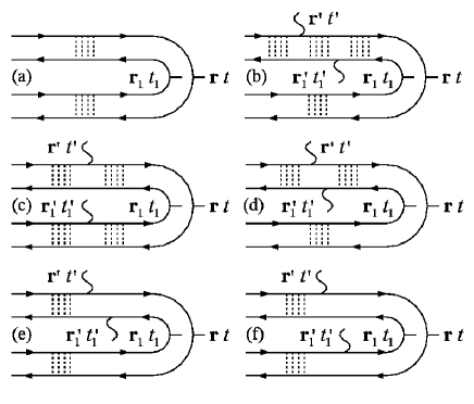
Figure 1: (a) Diagrammatic representation of the correlation function $\left<j_{\mathrm{ext}}^{(i)}({\mathbf{r}},t)j_{\mathrm{ext}}^{(j)}({\mathbf{r}}_{1},t_{1})\right>$ of Langevin currents ${\mathbf{j}}_{\mathrm{ext}}({\mathbf{r}},t)$. (b)–(d) Diagrams contributing to the correlation function $\left<q^{(i)}({\mathbf{r}},{\mathbf{r}}^{\,\prime},\Delta t)q^{(j)}({\mathbf{r}}_{1},{\mathbf{r}}^{\,\prime}_{1},\Delta t_{1})\right>$ of random response functions ${\mathbf{q}}({\mathbf{r}},{\mathbf{r}}^{\,\prime},\Delta t)$. (e) and (f) are examples of diagrams neglected in our analysis. Solid lines with right (left) arrows denote retarded (advanced) Green’s functions of the linear disordered wave equation. Dashed lines denote scattering of the two connected wave fields on the same heterogeneity. Wavy lines are $k_{0}^{2}$ vertices. The diagrams (b)–(f) are obtained by functional differentiation of the diagram (a) with respect to the dielectric constant of random medium.

In linear media, Langevin currents ${{\mathbf{j}}}_{\mathrm{ext}}({\mathbf{r}},t)$ are very sensitive to changes of disorder $\delta\varepsilon({\mathbf{r}})$ berk91 . Generalizing this property, one concludes that in a nonlinear medium ${{\mathbf{j}}}_{\mathrm{ext}}({\mathbf{r}},t)$ should be sensitive to changes of $\delta\varepsilon({\mathbf{r}})+\Delta\varepsilon_{\mathrm{NL}}({\mathbf{r}},t)$ spivak00 , and, more precisely, to changes of $\Delta\varepsilon_{\mathrm{NL}}({\mathbf{r}},t)$, since $\delta\varepsilon({\mathbf{r}})$ is fixed (and hence does not change) in our case. Modification $\Delta{{\mathbf{j}}}_{\mathrm{ext}}({\mathbf{r}},t)$ of Langevin currents due to an infinitesimal change $\Delta[\Delta\varepsilon_{\mathrm{NL}}({\mathbf{r}},t)]$ of the nonlinear part of dielectric constant is skip03a

$$\Delta{\mathbf{j}}_{\mathrm{ext}}({\mathbf{r}},t) = \int_{V}\mathrm{d}^{3}{\mathbf{r}}^{\,\prime}\int_{-\infty}^{t}\mathrm{d}t^{\,\prime}\,{\mathbf{q}}({\mathbf{r}},{\mathbf{r}}^{\,\prime},t-t^{\,\prime})$$ (5)

$$\times \Delta[\Delta\varepsilon_{\mathrm{NL}}({\mathbf{r}}^{\,\prime},t^{\,\prime})],$$

where the spatial integral is over the volume $V$ of the sample, we neglect the terms of the second and higher orders in $\Delta\varepsilon_{\mathrm{NL}}({\mathbf{r}},t)$, and ${\mathbf{q}}({\mathbf{r}},{\mathbf{r}}^{\,\prime},t-t^{\,\prime})$ are random, sample-specific response functions describing the sensitivity of Langevin currents ${\mathbf{j}}_{\mathrm{ext}}$ at ${\mathbf{r}}$ at time $t$ to small changes of dielectric constant $\varepsilon=1+\delta\varepsilon+\Delta\varepsilon_{\mathrm{NL}}$ at ${\mathbf{r}}^{\,\prime}$ at time $t^{\,\prime}$. (In general case, $\Delta[\Delta\varepsilon_{\mathrm{NL}}({\mathbf{r}}^{\,\prime},t^{\,\prime})]$ in Eq. (5) should be replaced by $\Delta\varepsilon({\mathbf{r}}^{\,\prime},t^{\,\prime})$, but we assume that the linear dielectric constant $1+\delta\varepsilon({\mathbf{r}})$ is fixed.) The physical meaning of ${\mathbf{q}}$ can be understood by considering a brief ‘flash’ of $\varepsilon$, $\Delta\varepsilon({\mathbf{r}},t)\propto\delta({\mathbf{r}}-{\mathbf{r}}_{0})\,\delta(t-t_{0})$, that occurs at time $t_{0}$ and is localized at ${\mathbf{r}}_{0}$. According to Eq. (5), for $t>t_{0}$ such a flash will modify the Langevin current at some distant point ${\mathbf{r}}$ by $\Delta{\mathbf{j}}_{\mathrm{ext}}({\mathbf{r}},t)\propto{\mathbf{q}}({\mathbf{r}},{\mathbf{r}}_{0},t-t_{0})$. To account for changes of $\varepsilon$ throughout the whole disordered sample and at all times before the time $t$, one has to sum their associated $\Delta{\mathbf{j}}_{\mathrm{ext}}$, which results in integration over space and time and leads to Eq. (5).

Obviously, the mean value of ${\mathbf{q}}$ is zero, while the correlation function of its Cartesian components is given by a sum of diagrams (b)–(d) of Fig. 1:

$$\left<q^{(i)}({\mathbf{r}},{\mathbf{r}}^{\,\prime},\Delta t)q^{(j)}({\mathbf{r}}_{1},{\mathbf{r}}_{1}^{\,\prime},\Delta t_{1})\right>$$

$$=3\pi D^{2}(c^{2}/\ell)\delta_{ij}\delta({\mathbf{r}}-{\mathbf{r}}_{1})$$

$$\times\left\{\left<I({\mathbf{r}}^{\,\prime})\right>G({\mathbf{r}}^{\,\prime},{\mathbf{r}}_{1}^{\,\prime};\Delta t-\Delta t_{1})G({\mathbf{r}}_{1}^{\,\prime},{\mathbf{r}};\Delta t_{1})\left<I({\mathbf{r}})\right>\right.$$

$$+\left.\left<I({\mathbf{r}}_{1}^{\,\prime})\right>G({\mathbf{r}}_{1}^{\,\prime},{\mathbf{r}}^{\,\prime};\Delta t_{1}-\Delta t)G({\mathbf{r}}^{\,\prime},{\mathbf{r}};\Delta t)\left<I({\mathbf{r}})\right>\right.$$

$$-\left.\left<I({\mathbf{r}}^{\,\prime})\right>G({\mathbf{r}}^{\,\prime},{\mathbf{r}};\Delta t)\left<I({\mathbf{r}}_{1}^{\,\prime})\right>G({\mathbf{r}}_{1}^{\,\prime},{\mathbf{r}};\Delta t_{1})\right.$$

$$+\left.k^{2}\ell/(3\pi D)\delta(\Delta t-\Delta t_{1})f^{2}({\mathbf{r}}^{\,\prime}-{\mathbf{r}}_{1}^{\,\prime})\left<I({\mathbf{r}})\right>\right.$$

$$\times\left.\left[\left<I({\mathbf{r}}^{\,\prime})\right>G({\mathbf{r}}^{\,\prime},{\mathbf{r}};\Delta t)+\left<I({\mathbf{r}}_{1}^{\,\prime})\right>G({\mathbf{r}}_{1}^{\,\prime},{\mathbf{r}};\Delta t)\right]\right\}.$$ (6)

Each term in Eq. (6) and a corresponding diagram of Fig. 1 can be given a simple physical interpretation. Consider, for example, the first term, $\left<I({\mathbf{r}}^{\,\prime})\right>G({\mathbf{r}}^{\,\prime},{\mathbf{r}}_{1}^{\,\prime};\Delta t-\Delta t_{1})G({\mathbf{r}}_{1}^{\,\prime},{\mathbf{r}};\Delta t_{1})\left<I({\mathbf{r}})\right>$, given by the diagram (b) of Fig. 1. This term contains two wave fields $E$ and two complex conjugate fields $E^{*}$ that enter the disordered medium from the left. The first pair of $E$ and $E^{*}$, shown by two lower solid lines in Fig. 1(b), propagate together to the vicinity of points ${\mathbf{r}}$ and ${\mathbf{r}}_{1}$, experiencing scatterings at exactly the same scatterers (this is denoted by dashed horizontal lines). After the last scattering event, these two fields do not follow the same path anymore: $E$ goes to ${\mathbf{r}}_{1}$ and $E^{*}$ goes to ${\mathbf{r}}$. The second pair of $E$ and $E^{*}$, depicted by two upper solid lines in Fig. 1(b), propagate together to some intermediate point ${\mathbf{r}}^{\,\prime}$ where $E$ experiences scattering on a fluctuation $\Delta[\Delta\varepsilon_{\mathrm{NL}}({\mathbf{r}}^{\,\prime},t^{\,\prime})]$ of the nonlinear part of dielectric constant. The two wave fields then continue together to some other point ${\mathbf{r}}_{1}^{\,\prime}$, where $E^{*}$ is scattered by $\Delta[\Delta\varepsilon_{\mathrm{NL}}({\mathbf{r}}_{1}^{\,\prime},t_{1}^{\,\prime})]$. Finally, the two wave fields make the remaining way from ${\mathbf{r}}_{1}^{\,\prime}$ to the vicinity of points ${\mathbf{r}}$ and ${\mathbf{r}}_{1}$ together and then separate for $E$ to go to ${\mathbf{r}}$ and $E^{*}$ — to ${\mathbf{r}}_{1}$. Similar interpretation can also be given to other terms of Eq. (6) and to the diagrams (c)–(f) of Fig. 1. We note that the last term in Eq. (6) [the term containing the factor $f^{2}({\mathbf{r}}^{\,\prime}-{\mathbf{r}}_{1}^{\,\prime})$], given by the diagram (d) of Fig. 1, has been neglected in Ref. skip03a, . This is only justified in the limit of extremely large sample size and for very slow speckle dynamics as will be shown below. Also, it should be noted that there exist other diagrams that contribute to the correlation function $\left<q^{(i)}({\mathbf{r}},{\mathbf{r}}^{\,\prime},\Delta t)q^{(j)}({\mathbf{r}}_{1},{\mathbf{r}}_{1}^{\,\prime},\Delta t_{1})\right>$ but are neglected in our analysis. We show examples of such diagrams in panels (e) and (f) of Fig. 1. These two particular diagrams are neglected in Eq. (6) because their contribution to our principal result, Eq. (12), is a factor $(\ell/L)^{2}\ll 1$ smaller than the contribution of diagrams (b)–(d). In addition to neglecting non-leading diagrams in Eq. (6), we note that the diagrams (b) and (c) will enter further analysis with the assumption $\left|{\mathbf{r}}^{\,\prime}-{\mathbf{r}}_{1}^{\,\prime}\right|>\ell$. Taking into account the opposite possibility ($\left|{\mathbf{r}}^{\,\prime}-{\mathbf{r}}_{1}^{\,\prime}\right|\leq\ell$) is possible but would modify our final Eq. (12) only by additional terms that are a factor $\ell/L\ll 1$ or a factor $(k\ell)^{-1}\ll 1$ smaller than the terms due to $\left|{\mathbf{r}}^{\,\prime}-{\mathbf{r}}_{1}^{\,\prime}\right|>\ell$.

A dynamic equation for ${\mathbf{j}}_{\mathrm{ext}}({\mathbf{r}},t)$ can be obtained from Eq. (5) by assuming that the changes of Langevin currents and nonlinear dielectric constant entering into that equation take place during some time interval $\delta t$. We then divide both sides of the equation by $\delta t$ and take the limit of $\delta t\rightarrow 0$. This yields

$$\frac{\partial}{\partial t}{\mathbf{j}}_{\mathrm{ext}}({\mathbf{r}},t) = \int_{V}d^{3}{\mathbf{r}}^{\,\prime}\int_{0}^{\infty}d\Delta t\,{\mathbf{q}}({\mathbf{r}},{\mathbf{r}}^{\,\prime},\Delta t)$$ (7)

$$\times \frac{\partial}{\partial t}\Delta\varepsilon_{\mathrm{NL}}({\mathbf{r}}^{\,\prime},t-\Delta t).$$

To describe the temporal evolution of $\Delta\varepsilon_{\mathrm{NL}}({\mathbf{r}},t)$, we employ a Debye-type relaxation equation,

$$\tau_{\mathrm{NL}}\frac{\partial}{\partial t}\Delta\varepsilon_{\mathrm{NL}}({\mathbf{r}},t)=-\Delta\varepsilon_{\mathrm{NL}}({\mathbf{r}},t)+2n_{2}\delta I({\mathbf{r}},t),$$ (8)

which is commonly used in nonlinear optics to model the noninstantaneous medium response bloem96 ; boyd02 ; ikeda80 ; silber82 ; silber84 . Here the constant $n_{2}$ measures the strength of nonlinearity and the relaxation time $\tau_{\mathrm{NL}}$ characterizes the speed of nonlinear response of the medium. Note that we have subtracted from $\Delta\varepsilon_{\mathrm{NL}}({\mathbf{r}},t)$ in Eq. (8) its average value $2n_{2}\left<I({\mathbf{r}})\right>\ll 1$ that only leads to a small modification of the average refractive index of random medium and is of no significance in the context of the present study. Equations (3), (7) and (8) form a self-consistent system. Equation (3) governs the spatio-temporal evolution of the intensity fluctuations $\delta I({\mathbf{r}},t)$ due to the Langevin currents ${{\mathbf{j}}}_{\mathrm{ext}}({\mathbf{r}},t)$, Eq. (7) describes the distributed feedback mechanism, leading to variations of ${{\mathbf{j}}}_{\mathrm{ext}}({\mathbf{r}},t)$ depending on the changes of $\Delta\varepsilon_{\mathrm{NL}}({\mathbf{r}},t)$, and Eq. (8) relates $\Delta\varepsilon_{\mathrm{NL}}({\mathbf{r}},t)$ to $\delta I({\mathbf{r}},t)=I({\mathbf{r}},t)-\left<I({\mathbf{r}})\right>$. Note that Eq. (7) is a linearized equation: only the terms linear in $\Delta\varepsilon_{\mathrm{NL}}({\mathbf{r}},t)\ll 1$ are kept. As we show below, the linearized nature of Eq. (7) may result in the exponential growth of its solution with time, and in this sense Eqs. (3), (7), and (8) are analogous to the equations of linear stability analysis commonly used to study the stability of nonlinear systems gibbs85 ; arecchi99 . Hence, although Eqs. (3), (7), and (8) will allow us to study the stability of the speckle pattern and the typical time scales of spontaneous intensity fluctuations beyond the instability threshold, they cannot be used to determine the amplitude of these fluctuations.

III Linear stability analysis

Consider now an infinitesimal periodic excitation of the stationary speckle pattern: $\delta I({\mathbf{r}},t)=\delta I({\mathbf{r}},\nu)$ $\exp(i\nu t)$, where $\nu=\Omega-i\Lambda$. Such an excitation can be either damped or amplified, depending on the sign of the Lyapunov exponent $\Lambda$. The value of $\Lambda$ is determined by two competing processes: on the one hand, diffusion tends to smear the excitation out, while on the other hand, the distributed feedback sustains its existence. The mathematical description of this competition is provided by Eqs. (3), (7) and (8) that after the substitution of $\delta I({\mathbf{r}},t)=\delta I({\mathbf{r}},\nu)\exp(i\nu t)$ [and similarly for ${\mathbf{j}}_{\mathrm{ext}}({\mathbf{r}},t)$ and $\Delta\varepsilon_{\mathrm{NL}}({\mathbf{r}},t)$] become

$$i\nu\delta I({\mathbf{r}},\nu)-D\nabla^{2}\delta I({\mathbf{r}},\nu)=-{\mathbf{\nabla}}\cdot{{\mathbf{j}}}_{\mathrm{ext}}({\mathbf{r}},\nu),$$ (9)

$$i\nu{\mathbf{j}}_{\mathrm{ext}}({\mathbf{r}},\nu)=i\nu\int_{V}\mathrm{d}^{3}{\mathbf{r}}^{\,\prime}\int_{0}^{\infty}\mathrm{d}\Delta t\,{\mathbf{q}}({\mathbf{r}},{\mathbf{r}}^{\,\prime},\Delta t)$$

$$\hskip 56.9055pt\times\Delta\varepsilon_{\mathrm{NL}}({\mathbf{r}}^{\,\prime},\nu)\exp(-i\nu\Delta t),$$ (10)

$$i\nu\tau_{\mathrm{NL}}\Delta\varepsilon_{\mathrm{NL}}({\mathbf{r}},\nu)=-\Delta\varepsilon_{\mathrm{NL}}({\mathbf{r}},\nu)+2n_{2}\delta I({\mathbf{r}},\nu).\hskip 22.76219pt$$ (11)

If $\nu=0$, Eq. (9) yields the stationary, time-independent component of the speckle pattern, Eq. (10) is trivial, and Eq. (11) determines the time-independent part of the nonlinear dielectric constant (more precisely, its deviation from the average). This case is not of interest for us. From here on, we will consider the case of $\nu\neq 0$, because we are interested in dynamics of speckle pattern. We proceed by expressing $\Delta\varepsilon_{\mathrm{NL}}({\mathbf{r}},\nu)$ through $\delta I({\mathbf{r}},\nu)$ by using Eq. (11) and the correlation function $\left<\delta I({\mathbf{r}},\nu)\delta I^{*}({\mathbf{r}}_{1},\nu)\right>$ through $\left<j_{\mathrm{ext}}^{(i)}({\mathbf{r}},\nu)j_{\mathrm{ext}}^{(j)*}({\mathbf{r}}_{1},\nu)\right>$ by using Eq. (9). The latter correlation function can, in its turn, be expressed through $\left<\delta I({\mathbf{r}},\nu)\delta I^{*}({\mathbf{r}}_{1},\nu)\right>$ by using Eq. (10). The two resulting equations relating $\left<j_{\mathrm{ext}}^{(i)}({\mathbf{r}},\nu)j_{\mathrm{ext}}^{(j)*}({\mathbf{r}}_{1},\nu)\right>$ and $\left<\delta I({\mathbf{r}},\nu)\delta I^{*}({\mathbf{r}}_{1},\nu)\right>$ have to be consistent, which yields an equation for allowed values of $\Omega$ and $\Lambda$. The calculation can be performed along the same lines as in Ref. skip03a, and yields

$$p \simeq \frac{1+k\ell/(L/\ell)}{h(\Omega T_{D},\Lambda T_{D})+k\ell/(L/\ell)g(\Lambda T_{D})}$$ (12)

$$\times H(\Omega\tau_{\mathrm{NL}},\Lambda\tau_{\mathrm{NL}}),$$

where $\Delta n=n_{2}{\overline{\left<I({\mathbf{r}})\right>}}$ is a typical value of the nonlinear modification of refractive index (with bar denoting spatial average) and the dimensionless function $h$ is defined in Ref. skip03a, [Eq. (A10) of Ref. skip03a, with ${\mathbf{R}}=0$]. Instead of reproducing here a (rather lengthy) expression for $h(x,y)$, we only note that $h(0,0)=1$, $1-h(x,0)\propto x^{2}$ for $x\ll 1$ and $h(x,0)\propto x^{-1/2}$ for $x\gg 1$. Functions $H$ and $g$ in Eq. (12) are defined as $H(x,y)=x^{2}+(1+y)^{2}$ and

$$g(y) = \frac{2}{(2-3e^{-1/2})}\frac{1}{2y+1}\left[1-\left(1+\frac{1}{2}\sqrt{2y+1}\right)\right.$$ (13)

$$\times \left.\exp\left(-\frac{1}{2}\sqrt{2y+1}\right)\right].$$

Finally, in Eq. (12) we have introduced a bifurcation parameter

$$p=\Delta n^{2}\left(\frac{L}{\ell}\right)^{2}\left(k\ell+\frac{L}{\ell}\right).$$ (14)

As will be seen from the following, this parameter controls the stability of speckle pattern with respect to weak perturbations.

Different terms in Eq. (12) have precise physical meaning. Functions $h$ and $g$ describe the distributed feedback mechanisms due to long-range ($h$) and short-range ($g$) correlations of intensity fluctuations in random medium. As follows from Eq. (12), the relative role of these two feedback mechanisms is controlled by the parameter $k\ell/(L/\ell)$. The fact that the nonlinear response of the medium is noninstantaneous is described by the function $H$. $H\equiv 1$ for $\tau_{\mathrm{NL}}=0$ and $H$ increases monotonically with both $\Omega$ and $\Lambda$ for $\tau_{\mathrm{NL}}>0$.

IV Instantaneous nonlinear response

We first illustrate the main result of the linear stability analysis performed in the previous section — Eq. (12) — on the most simple case of instantaneous nonlinearity, assuming $\tau_{\mathrm{NL}}=0$. In this case, $H\left(\Omega\tau_{\mathrm{NL}},\Lambda\tau_{\mathrm{NL}}\right)=1$ in Eq. (12). For every value of $p$ and a given $\Omega$ we can then solve Eq. (12) for $\Lambda$. If $\Lambda<0$, a weak harmonic (in time) excitation of speckle pattern at the chosen frequency $\Omega$ is exponentially suppressed and hence disappears after a time $\sim 1/\left|\Lambda\right|$. If, in contrast, $\Lambda>0$ our analysis predicts exponential amplification of the excitation and hence instability of speckle pattern with respect to weak perturbations at frequency $\Omega$. It follows from Eq. (12) that $\Lambda<0$ for all frequencies $\Omega$, if $p<1$. We illustrate this in Fig. 2 where we show a surface plot of $p$ versus $\Omega$ and $\Lambda$ for a particular case of $k\ell/(L/\ell)=1$. A thick line in Fig. 2 shows a crossection of the surface by a plane $\Lambda=0$ and splits the surface into two parts. All points with $\Lambda>0$ lie in the upper part of the surface and correspond to $p>1$. At higher $\Omega$, larger $p$ is required to get into the upper part of the surface. All points corresponding to $p<1$ belong to the lower part of the surface and correspond to $\Lambda<0$. When $p$ exceeds $1$, $\Lambda$ becomes positive in a band of frequencies $(0,\Omega_{\mathrm{max}})$ and speckle pattern is hence expected to exhibit instability with respect to low-frequency excitations. Thus, $p=1$ is the absolute instability threshold. This conclusion agrees with the result of Refs. skip00, and skip01, (where the same expression for the absolute instability threshold has been found by using a different approach) and coincides with the result of Ref. skip03a, in the limit of $L/\ell\gg k\ell$ considered in that paper. Equation (12) allows us to study dynamics of speckle pattern at $p>1$ and arbitrary $L/\ell$, $k\ell\gg 1$.

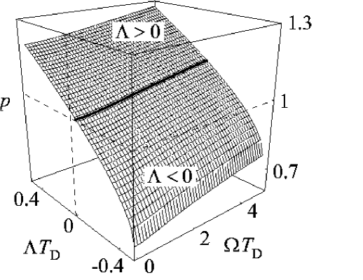
Figure 2: Stability diagram of speckle pattern in a nonlinear disordered medium. Physically realizable combinations of excitation frequency $\Omega$, Lyapunov exponent $\Lambda$ and bifurcation parameter $p$ belong to the surface shown in the figure. Thick line corresponds to $\Lambda=0$ and splits the surface into two parts. Instability ($\Lambda>0$) can only develop in the upper part of the surface and hence requires $p>1$. In the lower part of the surface, $p<1$ and $\Lambda<0$ for all $\Omega$.

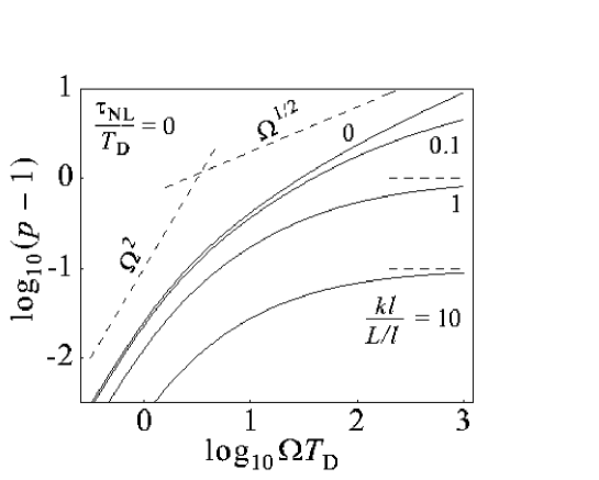
Figure 3: Frequency dependence of instability threshold in a nonlinear disordered medium with instantaneous Kerr nonlinearity ($\tau_{\mathrm{NL}}/T_{\mathrm{D}}=0$) for $k\ell/(L/\ell)\rightarrow 0$ (upper solid curve) and $k\ell/(L/\ell)=0.1$, 1, and 10 (solid curves from top to bottom). Inclined dashed lines show scaling laws $\Omega^{2}$ and $\Omega^{1/2}$. Horizontal dashed lines show asymptotic values of $p$ for large $\Omega$.

Frequency-dependent instability threshold (i.e. the value of $p$ at which $\Lambda=0$ for a given $\Omega$) is shown in Fig. 3 for several values of $k\ell/(L/\ell)$. If $k\ell/(L/\ell)\ll 1$ and $\Omega\ll\Omega_{1}=T_{\mathrm{D}}^{-1}[(L/\ell)/(k\ell)]^{2}$, which corresponds to the limit considered in Ref. skip03a, , the denominator of Eq. (12) is dominated by the first term $h(\Omega T_{D},\Lambda T_{D})$ and hence the threshold value of $p$ obeys scaling laws $p-1\propto(\Omega T_{\mathrm{D}})^{2}$ for $\Omega\ll T_{\mathrm{D}}^{-1}$ and $p\propto(\Omega T_{\mathrm{D}})^{1/2}$ for $T_{\mathrm{D}}^{-1}\ll\Omega\ll\Omega_{1}$ [see the curves corresponding to $k\ell/(L/\ell)=0$, $0.1$ and inclined dashed lines in Fig. 3]. This regime is governed by the presence of long-range correlations of intensity fluctuations [see Eq. (4)] and is mathematically described by the diagrams (b) and (c) of Fig. 1. The upper limiting frequency of the band inside which the speckle pattern is unstable (instability band) scales as $\Omega_{\mathrm{max}}\propto T_{\mathrm{D}}^{-1}(p-1)^{1/2}$ for $0<p-1\ll 1$ and as $\Omega_{\mathrm{max}}\propto T_{\mathrm{D}}^{-1}p^{2}$ for $p-1\gtrsim 1$. Note that $\Omega_{1}=T_{\mathrm{D}}^{-1}[(L/\ell)/(k\ell)]^{2}\sim(c/\ell)/(k\ell)^{2}$ exceeds $T_{\mathrm{D}}^{-1}$ for $L/\ell>k\ell$ but is still a factor $(k\ell)^{-2}\ll 1$ smaller than the inverse mean free time $c/\ell$. Therefore, our analysis applies for $\Omega\gtrsim\Omega_{1}$ as well. In this latter case, the second term, $k\ell/(L/\ell)g(\Lambda T_{D})$, in the denominator of Eq. (12) becomes larger than the first one and we find $p\simeq 1+(L/\ell)/(k\ell)$ (see dashed horizontal lines in Fig. 3). As one can see from Fig. 3, the curves corresponding to $k\ell/(L/\ell)=1$ and $10$ indeed tend to this asymptotic value for $\Omega>\Omega_{1}$. If $p$ exceeds $1+(L/\ell)/(k\ell)$, $\Lambda>0$ for all $\Omega$ and speckle pattern becomes unstable with respect to periodic excitations at all frequencies (in other words, $\Omega_{\mathrm{max}}\rightarrow\infty$). It is worthwhile to note that this wide-band instability is due to strong short-range correlations between intensity fluctuations in random media [see Eq. (2)] and mathematically results from the diagram (d) of Fig. 1. The short-range correlations appear to dominate the development of speckle pattern instability in relatively small random samples ($L/\ell\lesssim k\ell$, but still $L/\ell\gg 1$) and for high frequencies ($\Omega>\Omega_{1}$), while in large samples ($L/\ell\gg k\ell$) and for low frequencies ($\Omega<\Omega_{1}$) the principal role is played by the long-range correlations.

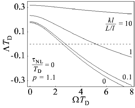
Figure 4: Lyapunov exponent $\Lambda$ versus excitation frequency $\Omega$ (both in units of $T_{\mathrm{D}}^{-1}=D^{2}/L$) in a nonlinear disordered medium with instantaneous Kerr nonlinearity ($\tau_{\mathrm{NL}}/T_{\mathrm{D}}=0$) slightly above the absolute instability threshold ($p=1.1$) for $k\ell/(L/\ell)\rightarrow 0$ (lower solid curve) and $k\ell/(L/\ell)=0.1$, 1, and 10 (solid curves from bottom to top). Horizontal dashed line shows $\Lambda=0$.

Lyapunov exponent $\Lambda$ as a function of frequency $\Omega$ can also be obtained from Eq. (12). For a system slightly above the absolute instability threshold ($p=1.1$), we plot corresponding results in Fig. 4 for the same values of $k\ell/(L/\ell)$ as in Fig. 3. In all cases, the maximal value of Lyapunov exponent $\Lambda_{\mathrm{max}}$ is reached for $\Omega\rightarrow 0$ and $\Lambda$ decreases monotonically with $\Omega$.

V Noninstantaneous nonlinear response

The case of instantaneous nonlinear response, $\tau_{\mathrm{NL}}=0$, considered in the previous section, is, obviously, not very realistic. In this section we extend the analysis of the previous section to arbitrary $\tau_{\mathrm{NL}}$. For concreteness, we fix the ratio $k\ell/(L/\ell)$ to a realistic value of $1$ and plot the frequency-dependent instability threshold resulting from Eq. (12) in Fig. 5. It is readily seen from the figure that the noninstantaneous nature of nonlinearity does not affect the absolute instability threshold $p=1$ but modifies significantly its frequency dependence. We have now several typical times (frequencies) that enter into play: the time $T_{\mathrm{D}}$ needed for a wave to diffuse through the random sample, the time $\tau_{\mathrm{NL}}$ of nonlinear response, and the time $\Omega_{1}^{-1}$, the inverse of the frequency at which the instability threshold saturates at a constant level in the case of instantaneous nonlinearity (corresponding typical frequencies are $T_{\mathrm{D}}^{-1}$, $\tau_{\mathrm{NL}}^{-1}$ and $\Omega_{1}$, respectively). In the particular case of $k\ell/(L/\ell)=1$ that we consider, $\Omega_{1}=T_{\mathrm{D}}^{-1}$.

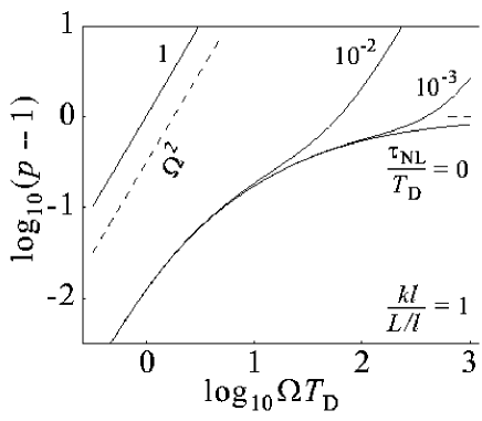
Figure 5: Frequency dependence of instability threshold in a nonlinear disordered medium with noninstantaneous Kerr nonlinearity ($\tau_{\mathrm{NL}}/T_{\mathrm{D}}=1$, $10^{-2}$ and $10^{-3}$, solid curves from top to bottom) compared with the case of instantaneous nonlinearity ($\tau_{\mathrm{NL}}/T_{\mathrm{D}}=0$, lower solid curve). $k\ell/(L/\ell)=1$ for all curves. Inclined dashed line shows scaling law $\Omega^{2}$, horizontal dashed line shows asymptotic value of $p$ for large $\Omega$ and $\tau_{\mathrm{NL}}/T_{\mathrm{D}}=0$.

Let us first assume that $\tau_{\mathrm{NL}}\ll T_{\mathrm{D}}$. For $\Omega\ll\tau_{\mathrm{NL}}^{-1}$, the behavior of instability threshold is then similar to that in the case of instantaneous nonlinearity (see Fig. 3 and the lower solid curve of Fig. 5). First, the threshold value of $p-1$ scales as $(\Omega T_{\mathrm{D}})^{2}$ for $\Omega<T_{\mathrm{D}}^{-1}$, then the curve starts to saturate at a constant level for $\Omega>\Omega_{1}$ [if $L/\ell>k\ell$ and $T_{\mathrm{D}}^{-1}<\Omega_{1}$, there is a region $T_{\mathrm{D}}^{-1}<\Omega<\Omega_{1}$, where $p\propto(\Omega T_{\mathrm{D}})^{1/2}$]. However, in contrast to the case of instantaneous nonlinearity, this saturation is not complete and is followed by a parabolic growth of $p$ with $\Omega$ for $\Omega>\tau_{\mathrm{NL}}^{-1}$. Physically, this is due to the fact that the nonlinear part of dielectric constant $\Delta\varepsilon_{\mathrm{NL}}$ cannot follow such fast dynamics and the amplitude of its oscillations is strongly suppressed for $\Omega>\tau_{\mathrm{NL}}^{-1}$. Mathematically, the growth of the threshold value of $p$ with $\Omega$ for $\Omega>\tau_{\mathrm{NL}}^{-1}$ originates from the term $H(\Omega\tau_{\mathrm{NL}},\Lambda\tau_{\mathrm{NL}})$ in Eq. (12). This behavior is illustrated by the solid curves corresponding to $\tau_{\mathrm{NL}}/T_{\mathrm{D}}=10^{-3}$ and $10^{-2}$ in Fig. 5.

If the response time of nonlinearity $\tau_{\mathrm{NL}}$ is of the order or shorter than $T_{\mathrm{D}}$ (see the upper solid curve in Fig. 5), the frequency dependence of instability threshold becomes dominated by the noninstantaneous nature of nonlinearity at all frequencies. We find $p-1\propto(\Omega\tau_{\mathrm{NL}})^{2}$ as illustrated in Fig. 5 for $\tau_{\mathrm{NL}}/T_{\mathrm{D}}=1$.

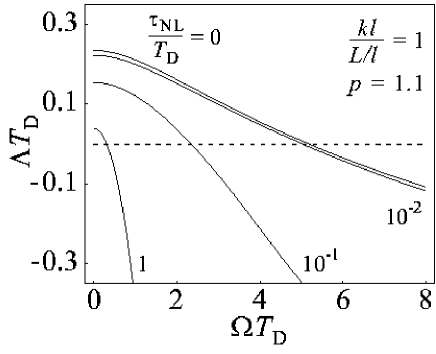
Figure 6: Lyapunov exponent $\Lambda$ versus excitation frequency $\Omega$ (both in units of $T_{\mathrm{D}}^{-1}=D^{2}/L$) in a nonlinear disordered medium with noninstantaneous Kerr nonlinearity ($\tau_{\mathrm{NL}}/T_{\mathrm{D}}=1$, $10^{-1}$ and $10^{-2}$, solid curves from bottom to top), slightly above the absolute instability threshold ($p=1.1$), compared to the case of instantaneous nonlinearity ($\tau_{\mathrm{NL}}/T_{\mathrm{D}}=0$, upper solid curve). $k\ell/(L/\ell)=1$ for all curves. Horizontal dashed line shows $\Lambda=0$.

The frequency dependence of Lyapunov exponent $\Lambda$ found by solving Eq. (12) slightly above the absolute instability threshold ($p=1.1$) and for $k\ell/(L/\ell)=1$ is shown in Fig. 6 for several values of $\tau_{\mathrm{NL}}/T_{\mathrm{D}}$. Qualitatively, behavior of $\Lambda$ is similar to that found in the case of instantaneous nonlinearity (see Fig. 4 and the upper solid curve of Fig. 6), but $\Lambda$ decreases with $\Omega$ faster than for $\tau_{\mathrm{NL}}/T_{\mathrm{D}}=0$. Together with a faster growth of instability threshold (Fig. 5), this narrows the band of frequencies $(0,\Omega_{\mathrm{max}})$ where excitations are subject to instability. Instead of becoming infinite for large $p$ as in the case of instantaneous nonlinearity ($\tau_{\mathrm{NL}}=0$), $\Omega_{\mathrm{max}}$ scales as $\tau_{\mathrm{NL}}^{-1}p^{1/2}$ for $\tau_{\mathrm{NL}}/T_{\mathrm{D}}\gg 1$.

VI Path-integral picture of speckle pattern instability

It is worth noting that most of the peculiarities of the above analysis can be qualitatively understood in the path-integral picture of wave propagation, especially in the case of instantaneous nonlinearity that we now consider in more detail.

Consider a partial wave traveling along a typical diffuse path of length $s\sim L^{2}/\ell$ in a nonlinear disordered medium. Assume that the path length $s$ can vary slowly with time due to, e.g., an infinitely slow Brownian motion of scatterers. A diffuse wave following the same path a time $\Delta t$ later will then acquire a different phase. The phase difference between the two waves, $\Delta\phi$, can be splited in a sum of two contributions: a ‘linear’ contribution $\Delta\phi_{\mathrm{L}}$, resulting directly from the change of path length $s$ and independent of the nonlinear properties of the medium, and a ‘nonlinear’ contribution $\Delta\phi_{\mathrm{NL}}$ due to the nonlinearity of the medium:

$$\Delta\phi_{\mathrm{NL}}=kn_{2}\int_{0}^{s}ds_{1}\Delta I({\mathbf{r}}),$$ (15)

where $\Delta I({\mathbf{r}})$ denotes the change of intensity during the time $\Delta t$, we take into account the fact that the nonlinear part of the refractive index is simply $n_{2}I({\mathbf{r}})$ in the considered case of instantaneous nonlinearity, and the integral is along the wave path. In the limit of weak nonlinearity, it can be shown skip01 ; skip03c that the mean values of both $\Delta\phi_{\mathrm{L}}$ and $\Delta\phi_{\mathrm{NL}}$ are zeroes, while their variances are related by

$$\left<\Delta\phi_{\mathrm{NL}}^{2}\right> = \left<\Delta\phi_{\mathrm{L}}^{2}\right>k^{2}n_{2}^{2}$$ (16)

$$\times \int_{0}^{s}ds_{1}\int_{0}^{s}ds_{2}\left<\delta I({\mathbf{r}}_{1})\delta I({\mathbf{r}}_{2})\right>,$$

where both integrals are along the same diffusion path. Because we have assumed nonlinearity to be weak, we can proceed by perturbation and replace the correlation function of intensity fluctuations $\left<\delta I({\mathbf{r}}_{1})\delta I({\mathbf{r}}_{2})\right>$ in Eq. (16) by its value in the linear medium, i.e., by a sum of two contributions: the short-range one [Eq. (2)] and the long-range one [Eq. (4)]. To perform integration in Eq. (16), we replace $\Delta r=\left|{\mathbf{r}}_{1}-{\mathbf{r}}_{2}\right|$ in the expression (2) for the short-range correlation function by $\Delta s=\left|s_{1}-s_{2}\right|$, assuming the wave path to be ballistic at distances shorter than $\ell$. In contrast, for $\Delta r>\ell$ the wave path is diffusive, and hence $\Delta r$ in the expression (4) for the long-range correlation function should be substituted by $(\Delta s\ell)^{1/2}$. Performing then integrations in Eq. (16) yields

$$\left<\Delta\phi_{\mathrm{NL}}^{2}\right>\simeq p\left<\Delta\phi_{\mathrm{L}}^{2}\right>,$$ (17)

with $p$ the bifurcation parameter defined by Eq. (14) with the first term, $\Delta n^{2}(L/\ell)^{2}k\ell$, resulting from the substitution of the short-range correlation function (2) in Eq. (16) and the second term, $\Delta n^{2}(L/\ell)^{3}$, — from the substitution of the long-range correlation function (4). It follows from Eq. (17) that at $p>1$, the phase difference $\Delta\phi=\Delta\phi_{\mathrm{L}}+\Delta\phi_{\mathrm{NL}}$ is dominated by $\Delta\phi_{\mathrm{NL}}$ and hence one may expect new phenomena (such as instability) to appear. Because we have already shown that $p=1$ is indeed the instability threshold, we adopt $\left<\Delta\phi_{\mathrm{NL}}^{2}\right>>\left<\Delta\phi_{\mathrm{L}}^{2}\right>$ as the instability condition within our path-integral picture.

The path-integral picture of wave propagation can be also applied to describe the dependence of instability threshold on the frequency of excitation. Indeed, assume that speckle pattern oscillates at some frequency $\Omega$ that (we remind) is assumed to be much smaller than the inverse mean free time $c/\ell$. At low frequencies $\Omega\ll T_{\mathrm{D}}^{-1}$ we recover Eq. (17) because the oscillations are very slow and everything happens as if the speed of light diffusion through the random medium were infinite. If, in contrast, $\Omega>T_{\mathrm{D}}^{-1}$, situation changes. In Eq. (16), the result of integration of the short-range correlation function (2) remains the same as before since this correlation is only non-zero for $\Delta r<\ell$ and $\Omega^{-1}$ is still much larger than the time needed for light to cover this distance. In contrast, integration of the long-range correlation function (4) now yields a different result. Indeed, in this case correlation between intensities at ${\mathbf{r}}_{1}$ and ${\mathbf{r}}_{2}$ can only be non-zero for $\Delta r=\left|{\mathbf{r}}_{1}-{\mathbf{r}}_{2}\right|\leq(D\Omega^{-1})^{1/2}<L$ due to the finite speed of light diffusion in random medium. Integration in Eq. (16) is therefore limited to pairs of points ${\mathbf{r}}_{1}$, ${\mathbf{r}}_{2}$ separated not more than by a distance $(D\Omega^{-1})^{1/2}$. This gives

$$\left<\Delta\phi_{\mathrm{NL}}^{2}\right>\simeq\Delta n^{2}\left(\frac{L}{\ell}\right)^{2}\left[k\ell+\frac{L}{\ell}\left(\Omega T_{\mathrm{D}}\right)^{-1/2}\right]\left<\Delta\phi_{\mathrm{L}}^{2}\right>.\hskip 8.53581pt$$ (18)

The condition of instability of speckle pattern with respect to excitations at frequency $\Omega$, $\left<\Delta\phi_{\mathrm{NL}}^{2}\right>>\left<\Delta\phi_{\mathrm{L}}^{2}\right>$, can now be written as

$$p\gtrsim\frac{1+k\ell/(L/\ell)}{(\Omega T_{D})^{-1/2}+k\ell/(L/\ell)}.$$ (19)

This coincides with Eq. (12) for $\Omega>T_{\mathrm{D}}^{-1}$.

The path-integral picture of speckle pattern instability can help to understand how to apply the theoretical model developed in this paper to realistic experimental situations, when the disordered sample is characterized by three different size parameters $L_{x}$, $L_{y}$, and $L_{z}$ (in the so-called ‘slab’ geometry, for example, $L_{x}=L_{y}\gg L_{z}\gg\ell$). In this case, the only size parameter $L$ of our theoretical model should be understood as a size of the part of disordered sample explored by a typical diffuse path (and hence $L\approx L_{z}$ in the slab geometry).

VII Discussion and conclusions

Theoretical analysis performed in the present paper indicates that the multiple-scattering speckle pattern in a nonlinear random medium with intensity-dependent dielectric constant becomes unstable with respect to weak dynamic perturbations if the nonlinearity exceeds the threshold $p\simeq 1$. This absolute instability threshold appears to be independent of the nonlinearity response time $\tau_{\mathrm{NL}}$, whereas the frequency dependence of the threshold (and, in particular, the spectrum of frequencies subject to instability) is very sensitive to $\tau_{\mathrm{NL}}$. It is pertinent to note the extensive nature of the bifurcation parameter $p$. According to Eq. (14), weak nonlinearity can be efficiently compensated by a sufficiently large sample size $L$ and $p\sim 1$ can be reached even at vanishing $\Delta n$, provided that $L$ is large enough. Another remarkable feature of Eq. (14) is the independence of $p$ of the sign of $\Delta n$. The phenomenon of speckle pattern instability is therefore expected to develop in a similar way for both positive and negative nonlinear coefficients $n_{2}$. This is not common for instabilities in nonlinear optical systems without disorder bloem96 ; boyd02 ; gibbs85 ; arecchi99 ; voron99 ; ikeda80 ; naka83 ; silber82 ; silber84 ; soljacic00 ; kip00 since the latter instabilities are often related to the self-focusing effect, arising at $n_{2}>0$ only. The instability discussed in the present paper is of different type and has nothing to do with self-focusing (which is negligible for $\Delta n^{2}k\ell\ll 1$ assumed throughout the paper). This does not mean, however, that phenomena similar to those discussed in the present paper do not exist in homogeneous nonlinear media. In fact, it is easy to see that Eq. (15) describes nothing but the self-phase modulation boyd02 of the multiple-scattering speckle pattern. The development of self-phase modulation in a random medium, however, appears to be rather different from that in the homogeneous case. Indeed, in a homogeneous medium of size $L$ the nonlinear phase shift is deterministic and $\phi_{\mathrm{NL}}=kn_{2}I_{0}L$ for a wave of intensity $I_{0}$, whereas in the case of diffuse multiple scattering $\phi_{\mathrm{NL}}$ is random with the average value $\left<\phi_{\mathrm{NL}}\right>\simeq kn_{2}I_{0}(L^{2}/\ell)$ and variance $\left<\phi_{\mathrm{NL}}^{2}\right>-\left<\phi_{\mathrm{NL}}\right>^{2}\simeq p$. The threshold of the speckle pattern instability $p\simeq 1$ can be therefore viewed as simply the point where the sample-to-sample fluctuations of the nonlinear phase shift become of order unity.

It is worth while to comment on the connection of the problem considered in the present paper to the recent results on modulational instability (MI) of incoherent light beams in homogeneous nonlinear media soljacic00 ; kip00 . In this case, a 2D speckle pattern (speckled beam) with a controlled degree of spatial and temporal coherence is ‘prepared’ by sending a coherent laser beam on a rotating diffuser. The beam is then incident on a homogeneous nonlinear medium (inorganic photorefractive crystal). Pattern formation and ‘optical turbulence’ are observed if the intensity of the beam exceeds a specific threshold, determined by the degree of coherence of the beam. Although the study presented in this paper is also concerned with the instability of speckle patterns in nonlinear media, it differs essentially from that of Refs. soljacic00, and kip00, at least in the following important aspects: (a) light loses its spatial coherence inside the medium, due to the multiple scattering on heterogeneities of refractive index, (b) the temporal coherence of incident light is perfect (in the case of incoherent MI soljacic00 ; kip00 , coherence time of the incident beam is much shorter than the nonlinearity response time $\tau_{\mathrm{NL}}$), and (c) the incident light beam is completely destroyed by scattering after a distance $\sim\ell$ and light propagation is diffusive in the bulk of the sample.

Let us now say a few words about practical consequences of our results and conditions of possible experimental observation of the instability phenomenon for light in random media. In a real experiment, infinitely weak dynamic perturbations of stationary speckle pattern are always present (due to, e.g., various types of noise). Our analysis predicts that the spectral components of these perturbations falling within the instability band $(0,\Omega_{\mathrm{max}})$ will be amplified due to the nonlinearity of the medium. Because our analysis is based on a linearized equation (7), we cannot predict further development of speckle dynamics with certainty, but our results suggest the following scenario. In general, there are two possibilities for the spontaneous dynamics of speckle pattern beyond the threshold. First, it can be (quasi-) periodic, i.e. dominated by oscillations at some discrete frequency (or frequencies) $\Omega_{i}$. Second, it can be chaotic with a continuous spectrum of intensity fluctuations between some $\Omega_{\mathrm{min}}$ and $\Omega_{\mathrm{max}}$. In nonlinear systems where dynamics is periodic, the frequency of oscillations $\Omega_{i}$ is often favored already on the level of the linear stability analysis: it is often the frequency for which the maximum Lyapunov exponent $\Lambda$ is reached. In our case, $\Lambda$ exhibits monotonic decrease with $\Omega$ (see Figs. 4 and 6), favoring no particular frequency. We have therefore no reason to expect the first scenario and the speckle pattern $I({\mathbf{r}},t)$ is likely to exhibit chaotic dynamics immediately beyond the instability threshold. The spectrum of chaotic fluctuations of $I({\mathbf{r}},t)$ will be continuous and comprised between $\Omega_{\mathrm{min}}=0$ and $\Omega_{\mathrm{max}}$ that we have discussed above. We note, however, that our analysis assumes diffusion regime of wave propagation ($k\ell\gg 1$ and $L/\ell\gg 1$) and is likely to fail if the scattering is low-order ($L\lesssim\ell$) or if the regime of Anderson localization is approached ($k\ell\sim 1$). In the latter cases, the first scenario of instability development can be a plausible option.

Finally, experimental observation of instability of multiple-scattering speckle pattern will require, first of all, large enough sample size $L$ and as low absorption as possible (if the macroscopic absorption length $L_{\mathrm{a}}<L$, the effective size of the sample will be limited to $L_{\mathrm{a}}$ and one will not fully exploit the extensivity of instability threshold). In the absence of absorption (or for $L_{\mathrm{a}}\gtrsim L$), $\Delta n_{\mathrm{NL}}\sim 10^{-2}$ (realistic in nematic liquid crystals) and $L/\ell\sim 20$ will suffice to get $p\simeq 1$ and reach the instability threshold. We note that in liquid crystals, optical nonlinearity is due to reorientation of molecules under the influence of electric field of electromagnetic wave and hence is essentially noninstantaneous. This emphasizes the importance of including the noninstantaneous nature of nonlinear response in our analysis.

References

- (1) M.C.W. van Rossum and Th.M. Nieuwenhuizen, Multiple scattering of classical waves: microscopy, mesoscopy, and diffusion, Rev. Mod. Phys. 71, 313–371 (1999).
- (2) Waves and Imaging through Complex Media, edited by P. Sebbah (Kluwer Academic Publishers, Dordrecht, 2001).
- (3) Wave Scattering in Complex Media: From Theory to Applications, edited by B.A. van Tiggelen and S.E. Skipetrov (Kluwer Academic Publishers, Dordrecht, 2003).
- (4) B. Shapiro, Large intensity fluctuations for wave propagation in random media, Phys. Rev. Lett. 57, 2168–2171 (1986).
- (5) M.J. Stephen and G. Cwilich, Intensity correlation functions and fluctuations in light scattered from a random medium, Phys. Rev. Lett. 59, 285–287 (1987).
- (6) A.Yu. Zyuzin and B.Z. Spivak, Langevin description of mesoscopic fluctuations in disordered media, Sov. Phys. JETP 66, 560–566 (1987).
- (7) R. Pnini and B. Shapiro, Fluctuations in transmission of waves through disordered slabs, Phys. Rev. B 39, 6986–6994 (1989).
- (8) M.P. van Albada, J. F. de Boer, and A. Lagendijk, Observation of long-range intensity correlation in the transport of coherent light through a random medium, Phys. Rev. Lett. 64, 2787–2790 (1990).
- (9) A.Z. Genack, N. Garcia, and W. Polkosnik, Long-range intensity correlation in random media, Phys. Rev. Lett. 65, 2129–2132 (1990).
- (10) P. Sebbah, B. Hu, A.Z. Genack, R. Pnini, and B. Shapiro, Spatial-field correlation: The building block of mesoscopic fluctuations, Phys. Rev. Lett. 88, 123901 (2002).
- (11) F. Scheffold, W. Härtl, G. Maret, and E. Matijević, Observation of long-range correlations in temporal intensity fluctuations of light, Phys. Rev. B 56, 10942–10952 (1997).
- (12) B. Shapiro, New type of intensity correlation in random media, Phys. Rev. Lett. 83, 4733–4735 (1999).
- (13) S.E. Skipetrov and R. Maynard, Nonuniversal correlations in multiple scattering Phys. Rev. B 62, 886–891 (2000).
- (14) I. Freund, M. Rosenbluh, and S. Feng, Memory effects in propagation of optical waves through disordered media, Phys. Rev. Lett. 61, 2328–2331 (1988).
- (15) F. Scheffold and G. Maret, Universal conductance fluctuations of light, Phys. Rev. Lett. 81, 5800–5803 (1998).
- (16) G. Maret and P.-E. Wolf, Multiple light scattering from disordered media. The effect of Brownian motion of scatterers, Z. Phys. B 65, 409–413 (1987).
- (17) D.J. Pine, D.A. Weitz, P.M. Chaikin, and E. Herbolzheimer, Diffusing wave spectroscopy, Phys. Rev. Lett. 60, 1134–1137 (1988).
- (18) R. Berkovits, Sensitivity of the multiple-scattering speckle pattern to the motion of a single scatterer, Phys. Rev. B 43, 8638–8640 (1991).
- (19) F. Scheffold, S. Romer, F. Cardinaux, H. Bissig, A. Stradner, V. Trappe, C. Urban, S. Skipetrov, L. Cipelleti and P. Schurtenberger, New trends in optical microrheology of complex fluids and gels, Prog. Colloid Polym. Sci., to appear.
- (20) A. Yodh and B. Chance, Spectroscopy and imaging with diffusing light, Phys. Today 48(3), 34–40 (1995).
- (21) D.S. Wiersma and A. Lagendijk, Light diffusion with gain and random lasers, Phys. Rev. E 54, 4256–4265 (1996).
- (22) D.S. Wiersma and S. Cavalieri, Light emission: A temperature-tunable random laser, Nature 414, 708–709 (2001).
- (23) R. Pappu, B. Recht, J. Taylor, and N. Gershenfeld, Physical one-way functions, Science 297, 2026–2030 (2002).
- (24) N. Bloembergen, Nonlinear Optics (World Scientific, Singapore, 1996).
- (25) R.W. Boyd, Nonlinear Optics (Academic Press, New York, 2002).
- (26) H.M. Gibbs, Optical Bistability: Controlling Light With Light (Academic Press, New York, 1985).
- (27) F.T. Arecchi, S. Boccaletti, and P. Ramazza, Pattern formation and competition in nonlinear optics, Phys. Rep. 318, 1–83 (1999).
- (28) Self-Organization in Optical Systems and Applications in Information Technology, edited by M.A. Vorontsov and W.B. Miller (Springer Verlag, Berlin, 1999).
- (29) A.A. Sukhorukov, Yu.S. Kivshar, O. Bang, J.J. Rasmussen, and P.L. Christiansen, Nonlinearity and disorder: Classification and stability of nonlinear impurity modes, Phys. Rev. E 63, 036601 (2001).
- (30) A. Trombettoni, A. Smerzi, and A.R. Bishop, Discrete nonlinear Schrödinger equation with defects, Phys. Rev. E 67, 016607 (2003).
- (31) G.B. Al’tshuler, V.S. Ermolaev, K.I. Krylov, A.A. Manenkov, and A.M. Prokhorov, Self-transparency effects in heterogeneous nonlinear scattering media and their possible use in lasers, J. Opt. Soc. Am. B 3, 660 (1986).
- (32) P. Sebbah, P. Sixou, C. Vanneste, and H. Guillard, Nonlinear scattering and optical power limitation in direct and inverse polymer dispersed liquid crystal, Nonlinear Optics 27, 377 (2001).
- (33) V.M. Agranovich and V.E. Kravtsov, Nonlinear backscattering from opaque media, Phys. Rev. B 43, 13691–13694 (1991).
- (34) V.E. Kravtsov, V.M. Agranovich, and K.I. Grigorishin, Theory of second-harmonic generation in strongly scattering media, Phys. Rev. B 44, 4931–4942 (1991).
- (35) J.F. de Boer, A. Lagendijk, R. Sprik, and S. Feng, Transmission and reflection correlations of second harmonic waves in nonlinear random media, Phys. Rev. Lett. 71, 3947–3950 (1993).
- (36) A.J. van Wonderen, Diagrammatic treatment of light scattering by a collection of Kerr particles, Phys. Rev. B 50, 2921–2940 (1994).
- (37) R. Bressoux and R. Maynard, On the speckle correlation in nonlinear random media, Europhys. Lett. 50, 460–465 (2000).
- (38) B. Spivak and A. Zyuzin, Mesoscopic sensitivity of speckles in disordered nonlinear media to changes of the scattering potential, Phys. Rev. Lett. 84, 1970–1973 (2000).
- (39) S.E. Skipetrov and R. Maynard, Instabilities of waves in nonlinear disordered media, Phys. Rev. Lett. 85, 736–739 (2000).
- (40) S.E. Skipetrov, Temporal fluctuations of waves in weakly nonlinear disordered media, Phys. Rev. E 63, 056614 (2001).
- (41) S.E. Skipetrov, Langevin description of speckle dynamics in nonlinear disordered media, Phys. Rev. E 67, 016601 (2003).
- (42) K. Ikeda, H. Daido, and O. Akimoto, Optical turbulence: Chaotic behavior of transmitted light from a ring cavity, Phys. Rev. Lett. 45, 709–712 (1980).
- (43) H. Nakatsuka, S. Asaka, H. Itoh, K. Ikeda, and M. Matsuoka, Observation of bifurcation to chaos in an all-optical bistable system, Phys. Rev. Lett. 50, 109–112 (1983).
- (44) Y. Silberberg and I. Bar Joseph, Instabilities, self-oscillation, and chaos in a simple nonlinear optical interaction, Phys. Rev. Lett. 48, 1541–1543 (1982).
- (45) Y. Silberberg and I. Bar Joseph, Optical instabilities in a nonlinear Kerr medium, J. Opt. Soc. Am. B 1, 662–670 (1984).
- (46) M. Soljacic, M. Segev, T. Coskun, D.N. Christodoulides, and A. Vishwanath, Modulation instability of incoherent beams in noninstantaneous nonlinear media, Phys. Rev. Lett. 84, 467–470 (2000).
- (47) D. Kip, M. Soljacic, M. Segev, E. Eugenieva, and D.N. Christodoulides, Modulation instability and pattern formation in spatially incoherent light beams, Science 290, 495–498 (2000).
- (48) As regards the effect of noninstantaneous nature of nonlinearity on speckle dynamics, our first results has been announced in S.E. Skipetrov, Instability of speckle patterns in random media with noninstantaneous Kerr nonlinearity, Opt. Lett. 28, 646–648 (2003).
- (49) S.E. Skipetrov and R. Maynard, Diffuse waves in nonlinear disordered media, in Ref. bartsergey, , 75–97.