Interaction broadening of Wannier functions and Mott transitions in atomic BEC

Abstract

Superfluid to Mott-insulator transitions in atomic BEC in optical lattices are investigated for the case of number of atoms per site larger than one. To account for mean field repulsion between the atoms in each well, we construct an orthogonal set of Wannier functions. The resulting hopping amplitude and on-site interaction may be substantially different from those calculated with single-atom Wannier functions. As illustrations of the approach we consider lattices of various dimensionality and different mean occupations. We find that in three-dimensional optical lattices the correction to the critical lattice depth is significant to be measured experimentally even for small number of atoms. Finally, we discuss validity of the single band model.

I introduction

Numerous many-body phenomena have been recently demonstrated with Bose-Einstein condensates (BEC) in optical lattices orz ; grei ; grei1 . Number squeezing has been observed with ⁸⁷Rb atoms in a one-dimensional lattice of pancake-shaped wells orz , and superfluid to Mott-insulator transitions have been witnessed with such atoms in three-dimensional and one-dimensional optical lattices grei . Such transitions were predicted by theoretical studies based on the Bose-Hubbard model BH and by microscopic calculations of the model parameters for BEC in optical lattices jaks ; Java .

Very important question is whether it is possible to observe superfluid to Mott-insulator transitions for the mean occupation number $n$ larger or even much larger than one? Phenomenological single band Bose-Hubbard model indeed predicts such transitions. Previous calculations of the model parameters $J$, hopping amplitude, and $U$, on-site interaction, were based on the lowest band Wannier functions for a single atom in an optical lattice. Repulsive interaction between the atoms for $n>1$ may cause the wave function in each well to expand in all directions, not only affecting the on-site interaction $U$  oo but also strongly enhancing tunneling $J$ between neighboring wells. This is especially significant in lower dimensional lattices with transverse potential bigger than the lattice wells where large occupations can be achieved without substantial three-body collisional loss. In order to provide theoretical guidance for experimental observation of Mott transitions in such systems, it is very important to obtain accurate critical parameters of the lattice potential for lattice occupations beyond unity.

Here we show how to construct an orthogonal basis of Wannier functions with mean-field atomic interactions taken into account. We use it to obtain renormalized values of parameters $J$ and $U$, from which critical depth of the potential $V_{c}$ is calculated for various lattices of different dimensionality and mean occupation. For the cubic optical lattice with $n=2$ or larger, our result is noticeably larger than that calculated without taking into account interaction. This increase is more pronounced for the anisotropic cases with stronger lattice potentials in one or two directions. For the case of one-dimensional lattice of pancake-shaped wells orz or two-dimensional lattice of tubes grei1 , our results are several times larger than critical values calculated from one-atom Wannier functions. This is in agreement with the experimental findings that much higher lattice potentials are needed to reach the transition point in such cases.

Kohn developed variational approach to calculate electronic Wannier functions in crystals  kohn . We modify this procedure by minimizing on-site energy self-consistently taking into account interaction between atoms.

In the last section we address validity of the single-band Bose-Hubbard model constructed with variational Wannier functions. The conditions for the model to be valid need to be modified from those for a single particle case since the interaction between the particles alters the band structure substantially wuniu . For the model to be valid two conditions have to be fulfilled: (i) when the number of particles in a well changes by one the variational Wannier function should not change significantly and (ii) collective excitations of the atoms within each well should be less energetically favorable than atom hopping between the wells.

II Bose-Hubbard model and Wannier functions

For bosonic atoms located in the lattice potential $V({\bf r})$ and described by boson field operators $\psi({\bf r})$, the Hamiltonian field operator is

$$H=\int{d{\bf r}\psi^{\dagger}({\bf r})\left({-\frac{{\hbar^{2}}}{{2m}}\nabla^{2}+V({\bf r})}\right)}\psi({\bf r})$$

$$+\frac{1}{2}\frac{{4\pi a_{s}\hbar^{2}}}{m}\int{d{\bf r}}\psi^{\dagger}({\bf r})\psi^{\dagger}({\bf r})\psi({\bf r})\psi({\bf r}),$$ (1)

where $a_{s}$ is the atoms’ scattering length and $m$ is the mass. To illustrate our methods we use as an example isotropic cubic lattice. We assume that the boson field operator may be expanded as $\psi({\bf r})=\sum_{i}b_{i}W({\bf r}-{\bf r}_{i})$, where $b_{i}$ is the annihilation operator for an atom in the Wannier state of site ${\bf r}_{i}$. Substituting this expansion into the Hamiltonian we obtain a problem of lattice bosons. We consider the case when the number of atoms per cite $n_{i}$ fluctuates around average number $n$. This results in the standard Bose-Hubbard Hamiltonian

$$H=-J\sum_{\langle ij\rangle}b_{i}^{\dagger}b_{j}+\frac{U}{2}\sum_{i}n_{i}(n_{i}-1)+\sum_{i}n_{i}I,$$ (2)

where the effective on-site repulsion $U$, the hopping amplitude $J$ and the on-site single-atom energy $I$ are defined by

$$U = \frac{\partial^{2}f}{\partial n^{2}}$$ (3)

$$J = \int{d{\bf r}W^{*}({\bf r})\left[{-\frac{{\hbar^{2}}}{{2m}}\nabla^{2}+V({\bf r})}\right]}W({\bf r}+{\bf a}),$$ (4)

$$I = \int d{\bf r}W^{*}({\bf r})\left[-\frac{\hbar^{2}}{2m}\nabla^{2}+V({\bf r})\right]W({\bf r}),$$ (5)

where $g=4{\pi}a_{s}\hbar^{2}/m$ and ${\bf a}$ is the lattice vector. On-site energy $f$ is defined as

$$f=nI+U_{0}n(n-1)/2,$$ (6)

with the bare on-site interaction $U_{0}$

$$U_{0}=g\int d{\bf r}|W({\bf r})|^{4}.$$ (7)

We assumed that the Wannier function does not change much for small fluctuations of the number of atoms. Off-site interactions are also neglected.

In case of more than one atom per site the presence of other atoms does modify the Wannier function of an atom. Below we describe our strategy for its self-consistent calculation. We start with a trial wave function localized in each well, $g({\bf r}-{\bf r}_{i})$. A Wannier function corresponding to the lowest Bloch band may be constructed according to Kohn’s transformation:

$$W({\bf r})=\sum_{i}c_{i}g({\bf r}-{\bf r}_{i}),$$ (8)

$$c_{i}=\int{d{\bf k}\over(2\pi)^{3}}\frac{e^{i{\bf k}\cdot{\bf r}_{i}}}{\sqrt{G({\bf k})}},$$

where the integral is over the first Brillouin zone and

$$G({\bf k}) = \sum_{i}\int d{\bf r}g({\bf r})g({\bf r}-{\bf r}_{i})\cos({\bf k}\cdot{\bf r}_{i}).$$ (9)

For an odd Wannier function, the cosine function should be replaced by the sine function. One can show that such Wannier functions are normalized and are orthogonal to each other for different wells. We vary the trial function to minimize the on-site energy $f$ mini .

We note that another method to calculate the Wannier functions including interaction effects self-consistently may be used for small interactions. Starting with non-linear time-independent Gross-Pitaevskii equation

$$-\frac{\hbar^{2}}{2m}\nabla^{2}\psi({\bf r}) + \frac{4\pi\hbar^{2}a_{s}}{m}|\psi({\bf r})|^{2}\psi({\bf r})$$ (10)

$$+ V({\bf r})\psi({\bf r})=\mu(\bf k)\psi(r),$$

one may calculate periodic Bloch states $u{\bf{}_{k}(r})$ defined as

$$\psi_{k}({\bf r})=e^{i{\bf k\cdot r}}u{\bf{}_{k}(r})/\sqrt{N}.$$ (11)

by expanding them in Fourier series

$$u_{\bf k}(x)=\sum_{n}A_{n}^{\bf k}e^{i2n\pi x/a}$$ (12)

and solving nonlinear system of equations. Then, a set of Wannier wave functions for the band in question is defined by

$$W_{m}({\bf r}-{\bf a}) = L^{-1/2}\sum_{BZ}\psi_{m,k}({\bf r}-{\bf a})$$ (13)

$$= L^{-1/2}\sum_{BZ}\psi_{m,k}({\bf r})e^{-i{\bf k}\cdot{\bf a}}.$$

This procedure fails for large interactions because the bands develop loops and become not single-valued wuniu .

III Superfluid to Mott-insulator transitions

We consider three optical lattice systems which are relevant to experiments: (i) isotropic three-dimensional optical lattice, (ii) anisotropic three-dimensional lattices, and (iii) the situation when the lattice potential is present only in one or two directions and confinement in other directions is provided by relatively weak harmonic trap. Following standard practice, we will use the lattice period $\pi/k$, atomic mass $m$, and recoil energy $E_{r}=\hbar^{2}k^{2}/2m$ as the basic units.

Three pairs of counter-propagating laser beams with wavelength $2\pi/k$ propagating along three perpendicular directions create potential

$$V({\bf r})=V_{x}\sin^{2}(kx)+V_{y}\sin^{2}(ky)+V_{z}\sin^{2}(kz).$$ (14)

Isotropic cubic lattice is created by the beam of equal intensity. In this case $V_{x}=V_{y}=V_{z}=V_{0}$.

Anisotropic cubic lattices can be created by choosing intensity of one or two beam to be much large than other. In this case $V_{y}=V_{z}=V_{\perp}\gg V_{x}=V_{0}$ or $V_{z}=V_{\perp}\gg V_{y}=V_{x}=V_{0}$. Below we study the case when $\hbar\omega_{\perp}\gg\mu$, where $\mu$ is the chemical potential of the atoms, thus the weak optical lattice is effectively one-dimensional or two-dimensional and transverse motion is frozen to the ground state of the transverse confinement.

Transverse motion can also be decoupled in the experimentally relevant case when the lattice potential is present only in one or two directions and atoms are confined in other directions by relatively weak harmonic trap: $V_{T}({\bf r}_{\perp})=\frac{1}{2}m\omega_{\perp}^{2}r^{2}_{\perp}$.

According to existing experiments, in our calculations through this work, we choose the ⁸⁷Rb atoms in $F=2,m=2$ state with scattering length $a_{s}=5.8$ nm and the laser wavelength of 852 nm for the three- and two-dimensional lattices and 840 nm for the one-dimensional lattice. All numerical results are obtained using 21 lattice wells in each direction with periodic boundary condition. Convergence has been checked using 41 wells for some of the key results.

In each case we calculate parameters of the Bose-Hubbard model based on the variational approach described in the previous section. The critical condition for superfluid to Mott-insulator transition has been found approximately as

$$U/zJ=2n+1+2\sqrt{n(n+1)},$$ (15)

where $z$ is the number of the nearest neighbor sites sheshadri . By substituting the parameters into the critical condition, we can map out the critical potential strength as a function of mean occupation.

In the following, we report our findings for isotropic and anisotropic three-dimensional lattices, one-dimensional lattice of pancake wells, and two-dimensional lattice of tubes.

III.1 Isotropic cubic lattice

In the case of isotropic cubic lattice we choose variational trial function to be in the form $g({\bf r})=g(x)g(y)g(z)$, with $g(u)=(1+\alpha u^{2})e^{-u^{2}/\sigma^{2}}$, where $\alpha$ and $\sigma$ are variational parameters. Then the Wannier function must also be of the product form $W({\bf r})=w(x)w(y)w(z)$, with the one-dimensional functions $w(u)$ and $g(u)$ related by the one-dimensional version of Kohn’s transformation. All the three-dimensional integrals in Eq. (2)-(15) can then be reduced to one-dimensional ones, greatly simplifying the calculations.

Figure 1: Dependence of various interaction parameters on number of atoms for $V=35E_{r}$. $U$ and $U_{0}$ are defined by (3) and (7) respectively. The derivative in (3) is calculated by Chebyshev fitting to function $f$. Interaction parameter $U_{0S}$ calculated with single particle Wannier function is defined as $U_{0S}=g\int d{\bf r}|W_{0}({\bf r})|^{4}$, where $W_{0}({\bf r})$ is a single-atom Wannier function.

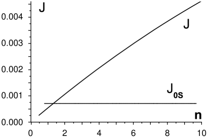
Figure 2: Hopping elements calculated with single particle Wannier function, $J_{0S}=\int{d{\bf r}W^{*}_{0}({\bf r})\left[{-\hbar^{2}\nabla^{2}/2m+V({\bf r})}\right]}W_{0}({\bf r+a})$, and with the variational proceedure described in the text, $J$. Depth of the lattice is $V=35E_{r}$.

Our calculations proceed as following. For a given $V_{0}$ and $n$, we start with certain initial parameters $\alpha$ and $\sigma$ to obtain a trial Wannier function through Kohn’s transformation and calculate the on-site energy $f$. The procedure is repeated by varying the parameters until the on-site energy $f$ is minimized. The resulting variational Wannier function will depend on both $n$ and $V_{0}$. If only the on-site single-atom energy $I$ is minimized, one obtains the single-atom Wannier function $W_{0}({\bf r})$ which only depends on $V_{0}$. We find that interaction broadens Wannier functions, as a result $U_{0s}$ is always larger than $U_{0}$, but we also notice that effective interaction $U$ can be larger than $U_{0}$ (see Fig. 1). So phase transition is more complex than we expected.

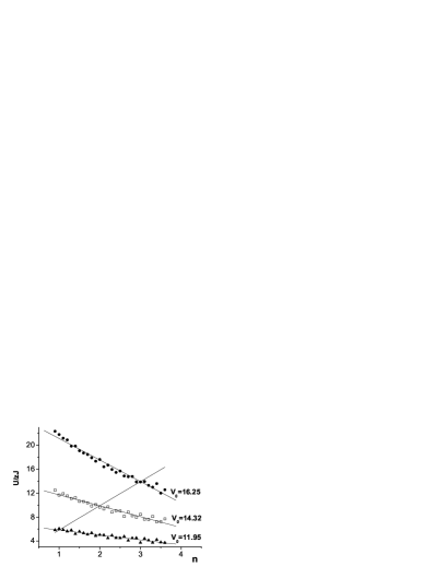
Figure 3: The ratio $U/zJ$ versus mean occupation $n$ calculated from the variational Wannier functions for isotropic cubic lattice. For each given parameter $V_{0}$, intersection with the solid line yields the mean occupation number for which the given $V_{0}$ is critical – condition in Eq.(15).

Once the Wannier function is determined, we can calculate the Bose-Hubbard parameters $U$ and $J$. In Fig. 3, we depict the ratio $U/zJ$ ($z=6$) as a function of the mean occupation $n$ for several values of the potential strength $V_{0}$. The decreasing trend can be understood as following. The total interaction energy increases with $n$, making the Wannier function broader, hence the interaction parameter $U$ becomes smaller, $J$ proportional to overlap between neighboring Wannier functions becomes larger, and as a result the ratio decreases. The intersection with the line of critical condition (in Fig. 3 the line with positive slope obtained from Eq. (15)) then yields the mean occupation for which these potentials are critical. For $n$=1,2,3 and 4, we find the critical potentials to be $V_{c}=11.95,14.32,16.25$ and $18.15$ respectively. A similar calculation can be done by using the a single-atom Wannier function. The critical potentials become $11.85,13.47,14.61$ and $15.43$ for the first four mean occupations. For $n=1$, the two results agree with each other within numerical uncertainty note3 , and are also consistent with experimentally determined range for the critical potential 2. For $n>1$, the mean field repulsion makes the critical potential noticeably higher. Starting from $n=3$ the correction to the critical depth of the lattice has to be clearly observable experimentally and effects of interaction has to be taken into consideration.

III.2 Anisotropic cubic lattices

Our procedure can also be applied to the case of an anisotropic lattice. We model the system as a lower dimensional problem with the reduced interaction parameter $g_{d}$ obtained by multiplying $g$ by the integral of $|\psi_{\perp}|^{4}$, where $\psi_{\perp}$ is the single-atom ground state wave function in a well of the transverse potential jaks . In the harmonic approximation, the wave function can be found exactly, and the reduced interaction parameter is given by $g_{1}=\frac{g\pi}{2}\sqrt{V_{\bot}}$ for the quasi-one-dimensional lattice and $g_{2}=g\sqrt{\frac{\pi}{2}}\sqrt[4]{V_{\bot}}$ for the quasi-two-dimensional lattice. In the calculations discussed below, we take $V_{\perp}=80E_{r}$.

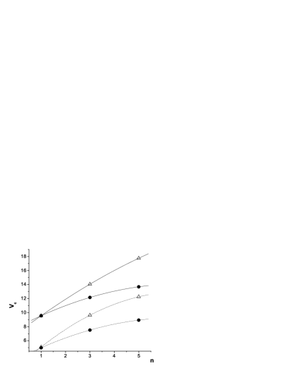
Figure 4: The critical lattice potential $V_{c}$ calculated from the variational and single-atom Wannier functions for anisotropic cubic lattices. The lines are guides to eyes. The dashed lines are for the quasi-one-dimensional and the solid lines are for quasi-two-dimensional cases. The triangles correspond to the variational and the circles to the single-particle calculations.

To find the Wannier functions for the lower dimensional lattices, we use these reduced interaction parameters in our procedure, replacing all the three-dimensional integrals in Eqs. (5) and (5) by lower dimensional ones. The critical lattice potential $V_{c}$ calculated using such variational Wannier functions is depicted in Fig. 4 for the one- and two-dimensional models. For comparison, we also include results calculated using the one-atom Wannier function. The increase of critical potential due to mean-field repulsion on the Wannier functions is somewhat bigger in the lower dimensional cases.

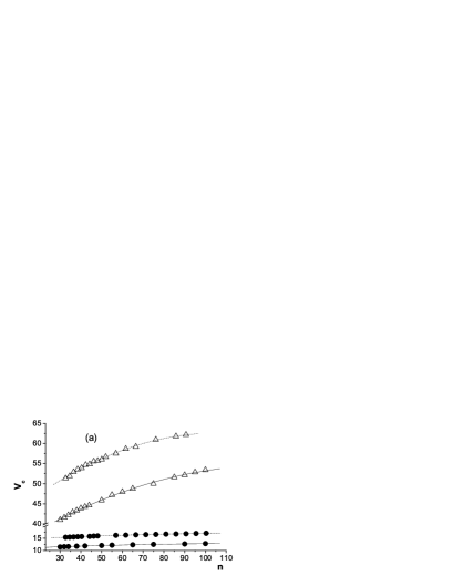
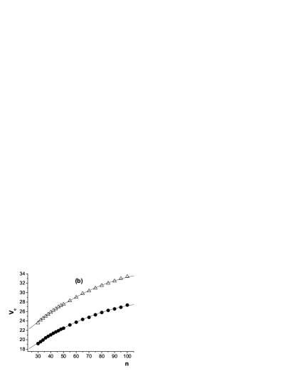
Figure 5: The critical lattice potential $V_{c}$ in dependence on mean occupation $n$ calculated from the variational (triangle) and single-atom (circle) Wannier functions for: (a) the one-dimensional lattice with $\omega_{\perp}=2\pi\times 19$ s^-1 (dashed line) and $\omega_{\perp}=2\pi\times 120$ s^-1 (solid line), and (b) two-dimensional lattice with $\omega_{\perp}=2\pi\times 24$ s^-1. The lines are guides to eyes.

III.3 Lattices in one or two directions

BECs in one-dimensional lattice of pancake-shaped wells and two-dimensional lattice of tube-shaped wells have been studied in experiments orz ; 3. Because of the large transverse dimensions of such wells, many atoms can be held in a well without suffering too much three-atom collisional loss, opening the possibility of studying superfluid/Mott-insulator transition for relatively large $n$ oo ; psg . In a theoretical investigation, Oosten et al oo considered the interaction effect by using a transverse wave function in the Thomas-Fermi approximation without modifying the single-atom Wannier function in the lattice direction(s). Here we extend their work by considering the interaction effect on the Wannier functions as well.

For the pancake like BEC array, the transverse wave functions are approximated by the Thomas-Fermi wave function $\phi_{TF}({\bf r_{\perp}})$ of the BEC within the pancake plane, which is defined by

$$|\phi_{TF}({\bf r_{\perp}})|^{2}=(ng_{1})^{-1}(\mu-V_{T}({\bf r}_{\perp})),$$ (16)

for $\mu>V_{T}({\bf r}_{\perp})=\frac{1}{2}m\omega_{\perp}^{2}r_{\perp}^{2}$ and vanishes otherwise. According to the experimental data, we take $\omega_{\perp}=19\times 2\pi s^{-1}$.

We begin by writing the Wannier function in the form, $W({\bf r})=w({\bf r}_{L})\phi({\bf r}_{\perp})$, where $\phi$ is the wave function for the transverse direction(s), and $w$ is the Wannier function in the lattice direction(s), both to be determined variationally by minimizing the on-site energy. The part of the on-site energy involving $\phi$ is just the $n$-particle Gross-Pitaevskii energy in the transverse potential and with the interaction parameter $g$ modified into $g_{d}$ by multiplying the integral of $|w({\bf r}_{L})|^{4}$. In the Thomas-Fermi approximation, this ‘transverse energy’ is given by $f_{\perp}={{2n-1}\over 3}\sqrt{nm\omega^{2}_{\perp}g_{1}/\pi}$ for the one-dimensional case and $f_{\perp}={{5n-2}\over 10}(9m\omega^{2}_{\perp}n^{2}g_{2}^{2})^{1/3}$ for the two-dimensional case. The total on-site energy is the sum of this ‘transverse energy’ and $n$ times of the single-atom energy of the lattice Wannier function:

$$f=f_{\perp}+n\int d{\bf r}_{L}w^{*}({\bf r}_{L})\left[-\frac{\hbar^{2}}{2m}\nabla^{2}+V({\bf r}_{L})\right]w({\bf r}_{L}).$$ (17)

Lattice Wannier function, obtained by the procedure of Kohn’s transformation and minimization of the on-site energy, will be affected by the interaction because the ‘transverse energy’ depends on it through the reduced interaction parameter $g_{d}$. After $w({\bf r}_{L})$ is determined variationally, the Bose-Hubbard parameters $J$ and $U$ can be calculated immediately. In Fig. 7, we show the critical potential $V_{c}$ for the case of one-dimensional lattice with transverse trap frequency $\omega_{\perp}/2\pi=19$ s^-1 and 120 s^-1.

For comparison, we also show the corresponding results obtained using the single-atom Wannier function of the lattice and the Thomas-Fermi transverse wave function. It is clear that $V_{c}$ is raised dramatically due to the broadening of the Wannier function. In the experiment of Ref. orz , the magnetic trap potential is 19 s^-1. The transverse trap frequency is enhanced to 120 s^-1 if the optical confining potential with $V_{0}=50E_{r}$ is turned on, and the mean occupation number is $n\sim 50$. Evidence from Bragg interference pattern shows that the critical value of the lattice potential should be somewhat larger than $44E_{r}$. This observation is contradictory to the prediction based on the single-atom Wannier function, but is consistent with our result based on the variational Wannier function.

In the case of two-dimensional lattice, our results for the critical lattice potential are shown in Fig. 7(b) for $\omega_{\perp}/2\pi=24$ s^-1 which is used in 3. We predict $V_{c}\sim 33E_{r}$ for $n\sim 100$, while the single-atom Wannier function yields $V_{c}\sim 27E_{r}$. The largest lattice potential used in the experiment was 12 $E_{r}$, so further experiment is needed to verify the theoretical predictions.

IV Validity of the single-band model

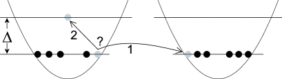
Figure 6: Energy associated with hopping (process 1) has to be smaller than energy to excite the many-body state in well (process 2). Many-body excitation is schematically depicted as a single atom excitation.

Figure 7: Relative change in the interaction energy as number of atoms changes by one determined by the change of the Wannier wave function.

In this section, we discuss the conditions for the single band Bose Hubbard model to be valid. First, we make general remarks and then give quantitative examples relevant for the case of the isotropic cubic lattice.

Assumption that the boson field operator may be expanded as $\psi({\bf r})=\sum_{i}b_{i}W({\bf r}-{\bf r}_{i})$ requires that the Wannier functions do not change substantially when the number of atoms in a well changes by one. A good criteria for this condition to be fulfilled is that interaction energy calculated with the Wannier function does not change much when number of particles changes by one

$$\frac{|U_{n}-U_{n+1}|}{U_{n}+U_{n+1}}\ll 1.$$ (18)

Note that the value of $U$ can still be quite different from the one calculated with a single particle Wannier function.

When the condition is fulfilled, the second condition is that the excitations within the ansatz have to be the least energetical. That is the hopping of the atoms from well has to be more energetically favorable than excitation of atoms in each well to the many-body excited state (see Fig. 6). If we consider two neighboring wells the energy of the ground state is

$$E_{0}=2nI+U_{0}n(n-1).$$ (19)

The energy associated with hopping is

$$\Delta E_{1}=2nI+U_{0}\frac{(n-2)(n-1)+n(n+1)}{2}-E_{0}=U_{0}.$$ (20)

It has to be much smaller than the energy of the first excited many-body state that we denote $\Delta$

$$U_{0}\ll\Delta.$$ (21)

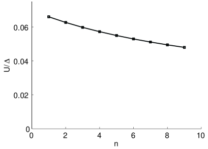
Figure 8: Ratio of the hopping energy to energy required to excite atoms in each well to the lowest many-body excited state.

We plot the criteria from Eq. (18) for isotropic lattices on Fig. 7. It is much smaller than unity. To estimate the effect of many-body excitation within a single well, we neglect hopping amplitude $J$, since close to Mott-insulator transition it is much smaller than atom’s interaction. Also for the experimentally relevant region of the potential depths the potential can be well approximated by a harmonic potential. In the harmonic potential the lowest many-body excited mode is associated with the center of mass motion – Kohn mode pethick . As a result $\Delta\sim\hbar\omega$. Since we neglect the tunneling we may start directly with variational form for the Wannier function in a well. We take $W(x,y,z)=W(x)W(y)W(z)$, where $W(u)=C(1+\beta u^{2})e^{-\gamma u^{2}}$. Similar to previous section for a fixed $V_{0}$ and $n$ we minimize on-site energy $f$. From the results shown in Fig. 8 it is clear that the single-band model is applicable in this case: the energy associated with atom’s hopping is much smaller than the energy required to excite the atoms inside of the wells.

The authors thank Dan Heinzen, Yu-Peng Wang, Shi-Jie Yang and Li You for the useful discussions. This work was supported in part by the National Science Foundation of China, the NSF of the United States, and the Welch Foundation of Texas.

References

- (1)
- (2) C. Orzel, A. K. Tuchman, M. L. Fenselau, M. Yasuda and M. A. Kasevich, Science 291, 2386 (2001).
- (3) M. Greiner, O. Mandel, T. Esslinger, T. W. Hänsch and I. Bloch, Nature 415, 39 (2002).T. Stöferle, H. Moritz, C. Schori, M. Köhl, T. Esslinger, Phys. Rev. Lett. 92, 130403(2004).
- (4) M. Greiner, I. Bloch, O. Mandel, T. W. Hänsch and T. Esslinger, Phys. Rev. Lett. 87, 160405 (2001);
- (5) M. P. A. Fisher, P. B. Weichman, G. Grinstein, and D. S. Fisher, Phys. Rev. B 40, 546 (1989).
- (6) D. Jaksch, C. Bruder, J. I. Cirac, C. W. Gardiner and P. Zoller, Phys. Rev. Lett. 81, 3108 (1998).
- (7) J. Javanainen, Phys. Rev. A 60, 4902 (1999).
- (8) D. van Oosten, P. van der Straten, and H. T. C. Stoof, Phys. Rev. A 67, 033606 (2003).
- (9) W. Kohn, Phys. Rev. B 7, 4388 (1973).
- (10) Biao Wu and Qian Niu, New Jour. of Phys. 5, 104 (2003).
- (11) According to Kohn kohn , minimization of the on-site energy for non-interacting particles does indeed give the correct Wannier functions for the lowest band, provided one starts with a sufficiently localized trial wave function of the correct symmetry.
- (12) W. Krauth, M. Caffarel, and J.-P. Bouchaud, Phys. Rev. B 45 3137 (1992); K. Sheshadri et al., Europhys. Lett. 22, 257 (1993); J. K. Freericks and H. Monien, Europhys. Lett. 26, 545 (1994).
- (13) The numerical errors come from optimizing the Wannier function, resulting in uncertainty of in . The result for is slightly lower than that reported in 2 based on single-atom Wannier function obtained from band structure calculations. In principle, our calculation can be made more precise by using more variational parameters in the trial functions (See, kohn ).
- (14) A. Polkovnikov, S. Sachdev and S. M. Girvin, Phys. Rev. A 66, 053607 (2002); E. Altman and A. Auerbach, Phys. Rev. Lett. 89, 250404 (2003).
- (15) Qian Niu, Modern Physics Letters B 5, 923 (1991).
- (16) C.J. Pethick and H. Smith, Bose-Einstein Condensation in dilute Gases (Cambridge University Press, Cambridge, 2002) Ch. 7.