Angular distribution of photoluminescence as a probe of Bose Condensation of trapped excitons

Abstract

Recent experiments on two-dimensional exciton systems have shown the excitons collect in shallow in-plane traps. We find that Bose condensation in a trap results in a dramatic change of the exciton photoluminescence (PL) angular distribution. The long-range coherence of the condensed state gives rise to a sharply focussed peak of radiation in the direction normal to the plane. By comparing the PL profile with and without Bose Condensation we provide a simple diagnostic for the existence of a Bose condensate. The PL peak has strong temperature dependence due to the thermal order parameter phase fluctuations across the system. The angular PL distribution can also be used for imaging vortices in the trapped condensate. Vortex phase spatial variation leads to destructive interference of PL radiation in certain directions, creating nodes in the PL distribution that imprint the vortex configuration.

The possibility of Bose condensation in two-dimensional exciton systems, such as coupled quantum wells, has been actively investigated recently [1, 2, 3, 4, 5, 6]. The interest in these systems is caused by relatively long recombination times that should make it possible to create a sufficiently cold system at high density, and thereby reach the condensation transition point. Further, their two dimensional nature leads to a repulsive interaction, disfavouring the formation of biexcitons. It was proposed that the condensation of excitons can be facilitated in the presence of in-plane traps [7]. Since the temperature of the exciton gas depends on the intensity of the laser used to pump excitons, it is advantageous if the excitons can reach critical density at lower pumping power. By collecting excitons in a trap, a lower total flux of excitons and hence a lower pumping power is required. Small traps of micron size arising due to ambient disorder [3] (see also [8]), as well as more shallow traps ca. hundred microns wide created artificially by stress [9] have been considered.

The density distribution of excitons in such relatively shallow traps (of the order of $1\,{\rm meV/\mu m}$) changes very little through the condensation transition. Thus, in contrast with the cold atom systems[10, 11], the direct spatial imaging of density is not expected to provide dramatic evidence for condensation. The principal manifestations of Bose condensation discussed to date include changes in PL spectrum [2, 12] and exciton recombination rate [1, 7].

In this work, we demonstrate that PL angular distribution can be used as a sensitive probe of Bose condensation in a trap. For excitons confined to move in a plane, in recombination momentum conservation perpendicular to this plane is relaxed. The intensity of radiation at a particular angle is therefore controlled by the distribution of in plane momenta of the excitons. Bose condensation produces large occupation of the state with zero velocity, thereby creating a peak in the momentum distribution, which gives rise to a sharp peak in the PL angular profile. Well below the transition, once the long-range order in the condensate extends across the entire exciton cloud in trap, the phases of the condensate order parameter become correlated throughout the cloud. This makes the PL radiation from different parts of the cloud fully coherent, and thus focussed in a cone with opening angle ca. $\lambda_{\rm rad}/L$, with $\lambda_{\rm rad}$ the optical wavelength and $L$ the cloud size.

To extract the PL angular profile, we consider dipole radiation of excitons, with momentum conservation perpendicular to the plane relaxed [13, 14],

$$I({\bf k}_{\parallel})\propto N_{\rm ex}({\bf k}_{\parallel})\rho_{\rm ph}({\bf k}_{\parallel},k_{0})\left|\left<f\right|{\bf k}_{\parallel}.\hat{{\bf p}}\left|i\right>\right|^{2}$$ (1)

where $k_{0}=2\pi/\lambda_{\rm rad}$ is photon wavenumber, $N_{\rm ex}({\bf k}_{\parallel})$ is the number of excitons with momentum ${\bf k}_{\parallel}$, $\rho_{\rm ph}({\bf k}_{\parallel},k_{0})$ the photon density of states, and $\left|i\right>$ and $\left|f\right>$ represent the initial and final electronic states. After $|{\bf k}_{\parallel}|$ is expressed in terms of the angle $\theta$ to the plane normal, $|{\bf k}_{\parallel}|=k_{0}\sin\theta$, the photon density of states and matrix element give a factor $(1+\cos^{2}\theta)/\cos\theta$.

The momentum distribution of excitons depends on the state of the Bose gas:

$$N_{\rm ex}({\bf k}_{\parallel})=\left<|\psi({\bf k}_{\parallel})|^{2}\right>=\sum_{{\bf r},{\bf r}^{\prime}}\left<\psi^{\ast}({\bf r})\psi({\bf r}^{\prime})\right>e^{i{\bf k}_{\parallel}.({\bf r}-{\bf r}^{\prime})}$$ (2)

We model the system as a gas of interacting bosons moving in an external trap potential $V(r)$,

$$H[\psi]=\int\left[\psi^{*}\left(-\frac{\nabla^{2}}{2m}+V({\bf r})-\mu\right)\psi+\frac{\lambda}{2}\left|\psi\right|^{4}\right]d^{2}{\bf r}$$ (3)

where $\lambda$ is a momentum independent interaction.

In the Thomas-Fermi approximation [15], with the system energy being a functional of local density only, one can look for the minimum of the energy (3) with the gradient term omitted. For an harmonic trap $V({\bf r})=\frac{1}{2}\alpha{\bf r}^{2}$ containing $N$ particles, this gives a parabolic distribution

$$\left|\psi({\bf r})\right|^{2}=\frac{2N}{\pi R^{4}}(R^{2}-{\bf r}^{2})\,,\quad R=\left({\frac{4\lambda N}{\pi\alpha}}\right)^{1/4},$$ (4)

while $\psi_{|{\bf r}|>R}=0$. The momentum space profile is

$$N_{\rm ex}({\bf k})=8\pi R^{2}N\left(\frac{\sin kR}{(kR)^{3}}-\frac{\cos kR}{(kR)^{2}}\right)^{2}$$ (5)

(for brevity, from here on we use ${\bf k}\equiv{\bf k}_{\parallel}$). Oscillations in the expression (5) result from the sharp edge of the Thomas-Fermi distribution (4).

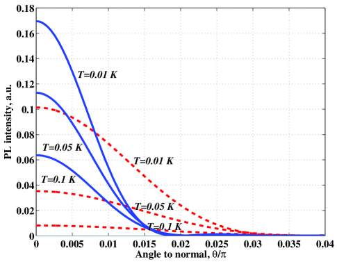
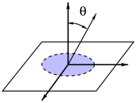
FIG. 1.: PL angular profile temperature dependence for particle number in the trap $N=10^{3}$ (solid lines) and $N=10^{2}$ (dashed lines). Temperature dependence is calculated for the parameters as discussed in the text, with $T_{\rm BEC}$ given by Eq.(6). The intensity for $N=10^{3}$ particles is reduced by a factor $1/20$ to allow comparison. Inset: PL radiation geometry of a 2D exciton cloud.

The momentum distribution (5) will produce a sharp peak in the PL angular profile if $R>\lambda_{\rm rad}$. For the indirect exciton line $\lambda_{\rm rad}\approx 800\,{\rm nm}$ [3]. By either considering the capacitance of such a device, or the momentum independent part of the Fourier transform of the interaction, we estimate that $\lambda=e^{2}d/\epsilon\approx 7.0\,{\rm nm^{2}eV}$ where $d\approx 5\,{\rm nm}$ is the inter-well spacing and $\epsilon$ the dielectric constant in GaAs.

A characteristic scale for the trap potential is $\alpha\approx 10^{-12}\,{\rm eV\,nm^{-2}}$ (i.e. $\Delta V=0.1\,{\rm meV}$ for $\Delta r=10\,{\rm\mu m}$, [3]). With these values, since the Thomas-Fermi radius $R\sim 1.5\,N^{1/4}{\rm\mu m}$, a peak should be visible even for small particle numbers.

The PL radiation geometry schematic and the peak, along with its temperature dependence discussed below, are shown in Fig.1.

The Bose condensation temperature can be estimated from the noninteracting model [3], $T_{\rm BEC}=\hbar\sqrt{\alpha N/gm}$, with $g=4$ the exciton degeneracy factor. Alternatively, since in a strongly interacting system the density change for $T<T_{\rm BEC}$ is small, $T_{\rm BEC}$ can be estimated from the degeneracy temperature at the density $\rho_{\rm max}$ of the centre of the Thomas-Fermi profile, giving

$$T_{\rm BEC}=\frac{2\pi\hbar^{2}}{m}\sqrt{\frac{N\alpha}{\lambda}}\approx 0.02\sqrt{N}\,[{\rm K}]$$ (6)

(for exciton mass $m=0.21\,m_{e}$, the value $m/2\pi\hbar^{2}=0.438\,{\rm nm^{-2}eV^{-1}}$). The two figures for $T_{\rm BEC}$ only differ by about a factor of $2$, because $\sqrt{\lambda m/2\pi\hbar^{2}}\approx 2$. With $N=10^{4}$ we obtain $T_{\rm BEC}\approx 2\,{\rm K}$. (This corresponds to an exciton density of $\sim 10^{-4}\,{\rm nm}^{-2}$, comfortably within the dilute limit.)

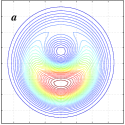
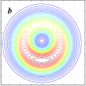
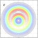
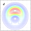
FIG. 2.: The correspondence between vortices and nodes in PL angular profile. Left to right: momentum distribution (2) for Thomas-Fermi condensate (4) with a single vortex (7) located on the $x$ axis at $x/R=-0.3,\,-0.1,\,0.1,\,0.3$. The off-center displacement of nodes in ${\bf k}$ space is $90^{\circ}$-rotated with respect to vortex displacement in position space.

The angular PL profile of the condensate changes in an interesting way in the presence of vortices. Here we study the momentum distribution for a condensate with $n$ vortices, and show that the vortices are ‘imaged’ by the nodes in ${\bf k}$-space. Consider the condensate (4) containing $n$ vortices. Using the complex variable $z=x+iy$ in the plane to write the phase factors due to the vortices located at the points $z_{j}$, we have

$$\psi_{n}({\bf r})=\psi_{0}({\bf r})\exp\left(i\sum_{j=1}^{n}{\rm arg}(z-z_{j})\right)$$ (7)

with $\psi_{0}$ defined by (4). Vortices give rise to nodes in the Fourier transform of $\psi_{n}({\bf r})$ and thereby in the momentum distribution $N_{\rm ex}({\bf k})$ (2). There is a one-to-one relation between the configuration of the nodes in $N_{\rm ex}({\bf k})$ and the vortex positions. Before discussing the more complicated case of phase vortices (7), it is instructive to look at an example of a condensate function of the form

$$\psi_{n}(z)=A\prod_{j=1}^{n}(z-z_{j})\exp\left(-\bar{z}z/2R^{2}\right)$$ (8)

describing $n$ ‘vortices’ with both the amplitude and phase varying in space. In this case the configuration of nodes in the momentum distribution is a very simple one. Evaluating the Fourier transform, we represent the polynomial $\prod_{j=1}^{n}(z-z_{j})$ as a differential operator, and obtain

$$\psi_{n}({\bf k}) = 2\pi A\prod_{j=1}^{n}(-2i\partial_{\bar{k}}-z_{j})\exp\left(-R^{2}\bar{k}k/2\right)$$ (9)

$$= 2\pi A\prod_{j=1}^{n}(iR^{2}k-z_{j})\exp\left(-R^{2}\bar{k}k/2\right)$$ (10)

with the complex variable $k=k_{x}+ik_{y}$. This expression has $n$ nodes at the points

$$k_{j}=-iz_{j}/R^{2}\,,\quad j=1,\ldots,n,$$ (11)

arranged in exactly the same way as vortices in real space, albeit rotated by $90^{\circ}$ in a clockwise direction.

Remarkably, the property that the pattern of the nodes in momentum distribution is a replica of the vortex arrangement, appears to be generic. Although the replica is exact only for ‘vortices’ of the form (8) and Gaussian density profiles, all the qualitative features hold also for the phase vortices (7). As an illustration, we consider a single phase vortex (7) located some distance $x$ away from trap center. As can be seen in Fig. 2, in this case there is exactly one node in momentum distribution, shifted off center by a distance that increases with $x$. The node displacement orientation is at a $90^{\circ}$ angle relative to the vortex displacement. A similar observation can be made for two vortices (Fig. 3a).

Also, we consider the configuration of nodes in $N_{\rm ex}({\bf k})$ corresponding to a vortex array of the form (7). Approximately, the nodes in this case also form a $90^{\circ}$-rotated array, with the distortion being a function of the inter-vortex spacing (Fig. 3b,c).

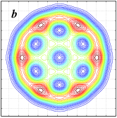
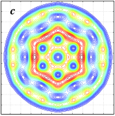
FIG. 3.: a) PL profile for $2$ vortices placed at $x/R=\pm 0.2$; b), c) PL profile for hexagonal arrays of 7 and 19 vortices. The insets show the configuration of vortices in real space.

Let us now turn to the discussion of finite temperature effects. At non-zero temperatures, in the presence of density and phase fluctuations, $\psi=\sqrt{\rho+\pi}e^{i\varphi}$, we construct a perturbation theory in $\pi$, $\varphi$. As discussed by Hohenberg and Fisher [16], who considered the perturbation expansion for weakly non-ideal Bose gas, this is only strictly valid at very low densities, $\ln(\ln(1/na^{2}))\gg 1$. Their renormalisation group analysis however suggests that no other interactions are relevant.

There are three temperature regimes, a low temperature part dominated by phase fluctuations, a free particle like regime, and a vortex dominated regime near the transition temperature. We consider only the phase fluctuations: it will become clear in a moment that the temperature dependence of the PL peak is predominantly due to the phase fluctuation effects. In this case, equation (2) becomes:

$$N_{\rm ex}({\bf k})=\sum_{{\bf r},{\bf r}^{\prime}}(\rho({\bf r})\rho({\bf r}^{\prime}))^{1/2}e^{-\frac{1}{2}D_{{\bf r},{\bf r}^{\prime}}}e^{i{\bf k}({\bf r}-{\bf r}^{\prime})}$$ (12)

with $D_{{\bf r},{\bf r}^{\prime}}=\left<\left(\varphi({\bf r})-\varphi({\bf r}^{\prime})\right)^{2}\right>$. The phase fluctuations are determined by the energy functional

$$H[\varphi]=\int\frac{\rho({\bf r})}{2m}\left(\nabla\varphi({\bf r})\right)^{2}d^{2}{\bf r}$$ (13)

so that the Green’s function $G({\bf r},{\bf r}^{\prime})=\left<\varphi({\bf r})\varphi({\bf r}^{\prime})\right>$ obeys

$$-\frac{\beta}{m}\nabla\left(\rho({\bf r})\nabla G({\bf r},{\bf r}^{\prime})\right)=\delta({\bf r}-{\bf r}^{\prime})$$ (14)

For a uniform density profile the solution is [17]

$$\frac{1}{2}\left<\left(\varphi({\bf r})-\varphi({\bf r}^{\prime})\right)^{2}\right>=\frac{m}{2\pi\beta\rho}\ln\left(\frac{|{\bf r}-{\bf r}^{\prime}|}{\xi_{T}}\right)$$ (15)

with the thermal length $\xi_{T}=(\lambda\rho/4m)^{1/2}/k_{\rm B}T$ corresponding to the energy cutoff in the Planck distribution of phase fluctuations.

One can use this result to estimate the fluctuation effect for the trapped gas. It is convenient to rewrite the logarithm so as to identify a separation dependent and an equal point term,

$$\frac{1}{2}\left(G({\bf r}^{\prime},{\bf r}^{\prime})+G({\bf r},{\bf r})-2G({\bf r},{\bf r}^{\prime})\right)=$$ (16)

$$-\frac{m}{2\pi\beta\rho}\left(\ln\left(\frac{\xi_{T}}{R}\right)-\ln\left(\frac{|{\bf r}-{\bf r}^{\prime}|}{R}\right)\right)$$ (17)

We consider in particular the case where ${\bf r}$ and ${\bf r}^{\prime}$ are well separated, so $G({\bf r},{\bf r}^{\prime})$ is small compared to $G({\bf r},{\bf r})$. (The typical separation ${\bf r}-{\bf r}^{\prime}$ in Eq.(12) is of the order of the cloud radius $R$.) In this case

$$N_{\rm ex}({\bf k})=\left|\int\sqrt{\rho({\bf r})}e^{-\frac{1}{2}G({\bf r},{\bf r})}e^{i{\bf k}.{\bf r}}d^{2}{\bf r}\right|^{2}$$ (18)

Physically, this result means that the phase fluctuations are dominated by the equal point contribution, which allows one to make a local density approximation in Eq.(16) and write $G({\bf r},{\bf r})=(m/2\pi\beta\rho({\bf r}))\ln(R/\xi_{T})$.

Let us now discuss the phase fluctuations more systematically, and verify the local density approximation. We shall consider the condensate in an harmonic trap. Returning to (14), rescaling ${\bf r}=R{\bf t}$, and using ${\bf t}$ as a new variable, $\rho(t)=\rho_{0}(1-t^{2})$, we write the solution to (14) as a sum of angular modes,

$$G({\bf t},{\bf t}^{\prime})=-\frac{m}{\beta\rho_{0}}\frac{1}{2\pi}\sum_{l=0}^{\infty}g_{l}(t,t^{\prime})e^{il(\theta-\theta^{\prime})}$$ (19)

The equation for mode $l$ has the form:

$$t^{2}(1-t^{2})\frac{d^{2}g_{l}}{dt^{2}}+t(1-3t^{2})\frac{dg_{l}}{dt}-l^{2}(1-t^{2})g=t\delta(t-t^{\prime})$$

The substitutions $g_{l}(t)=t^{\pm l}f(t)$ and $y=t^{2}$ show this is the hypergeometric equation [18], the general solution is

$$g_{l}(t,t^{\prime})=t^{l}_{<}h_{+l}(t_{<})\left[t^{l}_{>}h_{+l}(t_{>})-t^{-l}_{>}h_{-l}(t_{>})\right]$$ (20)

where $h$ is an hypergeometric function:

$$h_{\pm}(t)=F(a,b,c;t^{2})\,,\quad a+b=c=1\pm l,\quad ab=\pm l/2$$

and $t_{<}$($t_{>}$) correspond to the smaller(larger) of $t,t^{\prime}$.

As $t\rightarrow t^{\prime}$, the value of $G$ is dominated by the large $l$ terms, for which the functions $h_{\pm}(t)$ tend to $1/\sqrt{2|l|(1-t^{2})}$ and so we can consider the terms:

$$g_{l}(t+\epsilon,t-\epsilon)=\frac{1}{1-t^{2}}\frac{1}{2l}\left[t^{2l}\left\{1+{\mathcal{O}}\left(\epsilon^{2}\right)\right\}+\left(1-\frac{2l\epsilon}{t}\right)\right]$$

The second of the terms in brackets gives a divergence as $\epsilon\rightarrow 0$, of the form

$$\lim_{\epsilon\rightarrow 0}G(t+\epsilon,t-\epsilon) \approx \frac{-m}{\pi\beta\rho_{0}(1-t^{2})}\sum_{l=1}^{\infty}\frac{1}{2l}\left(1-\frac{\epsilon}{t}\right)^{2l}$$ (21)

$$= \frac{-m}{2\pi\beta\rho(t)}\ln\left(\frac{2\epsilon}{t}\right)$$ (22)

This matches both the nature of the divergence, and the pre-factor ($-m/2\pi\beta\rho$) seen in equation (16), and supports the local density approximation (18) for a finite system, with $\rho$ replaced by $\rho({\bf r})$.

From the asymptotes of the trapped gas Green’s functions (21), cutting the logarithmic divergence with the thermal length, the expression for momentum distribution due to far separated excitons (18) becomes:

$$N_{ex}({\bf k}_{\parallel})=\left|\int\left(\frac{\lambda\rho({\bf r})}{mR^{2}T^{2}}\right)^{mT/2\pi\rho({\bf r})}\!\!\!\sqrt{\rho({\bf r})}e^{i{\bf k}{\bf r}}d^{2}{\bf r}\right|^{2}$$ (23)

This expression has the form of replacing the condensate density with a “coherent particle density”,

$$\rho({\bf r})\rightarrow\rho({\bf r})\left(\frac{\rho({\bf r})}{\rho_{B}}\right)^{\rho_{A}/\rho({\bf r})}\\$$ (24)

For an harmonic trap, with the numbers discussed above,

$$\frac{\rho_{A}}{\rho_{0}}=\frac{mk_{\rm B}T}{8\pi\hbar^{2}}\sqrt{\frac{\pi\lambda}{2\alpha N}}\sim 30\times\frac{T[{\rm K}]}{\sqrt{N}}$$

$$\frac{\rho_{0}}{\rho_{B}}=\frac{\alpha 2\pi\hbar^{2}}{m(k_{\rm B}T)^{2}}\sim\left(\frac{10^{-2}}{T[{\rm K}]}\right)^{2}$$

The temperature dependence of the PL peak is shown in Fig.1. Qualitatively, the peak is suppressed at

$$T>T_{*}=T_{\rm BEC}/\ln(R/\xi_{T})$$ (25)

i.e. well below the condensation transition.

In summary, we propose that the angular profile of PL can be used as a diagnostic of Bose condensation in 2D exciton traps. A peak in the emission in a direction normal to the 2D plane appears due to long-range phase coherence in the condensate, at temperatures for which the coherence length exceeds the wavelength of the emitted radiation. The distribution of PL radiation in the peak is sensitive to the presence of phase textures in the condensate. In particular, vortices are imaged by the nodes in the PL angular profile.

We are grateful to L.V. Butov and B.D. Simons for useful discussions, and also for support from the Cambridge-MIT institute and the EU network “Photon-Mediated phenomena in semiconductor nanostructures” HPRN-CT-2002-00298. The NHMFL is supported by the National Science Foundation, the state of Florida and the US Department of Energy.

REFERENCES

- [1] L.V. Butov, A.L. Ivanov, A. Imamoglu, P.B. Littlewood, A.A. Shashkin, V.T. Dolgopolov, K.L. Campman, A.C. Gossard, Phys. Rev. Lett. 86, 5608 (2001)
- [2] A.V. Larionov, V.B. Timofeev, P.A. Ni, S.V. Dubonos, I. Hvam, K. Soerensen, JETP Lett. 75, 570 (2002).
- [3] L.V. Butov and C.W. Lai and A.L. Ivanov and A.C. Gossard and D.S. Chemla, Nature, 417, 47 (2002)
- [4] L.V. Butov, A.C. Gossard, D.S. Chemla, cond-mat/0204482; Nature 418, 751 (2002).
- [5] D. Snoke, S. Denev, Y. Liu, L. Pfeiffer, K. West, Nature 418, 754 (2002).
- [6] D. Snoke, Science 298, 1368 (2002). J. A. Kash, M. Zachau, E. E. Mendez, J. M. Hong, T. Fukuzawa Phys. Rev. Lett. 66, 2247 (1990)
- [7] L.V. Butov, A. Zrenner, G. Abstreiter, G. Böhm, G. Weimann, Phys. Rev. Lett. 73, 304 (1994)
- [8] L.V. Butov, L.S. Levitov, A.V. Mintsev, B.D. Simons, A.C. Gossard, D.S. Chemla, cond-mat/0308117, to be published
- [9] V. Negoita, D.W. Snoke and K. Eberl, Phys. Rev. B60, 2661 (1999)
- [10] E.A. Cornell, C.E. Wieman, Rev. Mod. Phys. 74, 875 (2002).
- [11] W. Ketterle, Rev. Mod. Phys. 74, 1131 (2002).
- [12] T. Fukuzawa, E. E. Mendez, J. M. Hong, Phys. Rev. Lett. 64, 3066 (1990),
- [13] L.C. Andreani, Sol. State Comm. 77, 641 (1991)
- [14] S.L. Chuang, Physics of Optoelectronic devices, (Wiley, 1995)
- [15] C.J. Pethick and H. Smith, Bose-Einstein Condensation in Dilute Gases, (Cambridge University Press, 2002)
- [16] D. Fisher and P. Hohenberg, Phys. Rev. B37, 4936 (1988)
- [17] V.N. Popov, Functional Integrals in Quantum Field Theory and Statistical Physics, (D. Reidel, 1983)
- [18] E. Whittaker and G. Watson, A course of Modern Analysis, (Cambridge University Press, 1927)