Split transition in ferromagnetic superconductors

Abstract

The split superconducting transition of up-spin and down-spin electrons on the background of ferromagnetism is studied within the framework of a recent model that describes the coexistence of ferromagnetism and superconductivity induced by magnetic fluctuations. It is shown that one generically expects the two transitions to be close to one another. This conclusion is discussed in relation to experimental results on URhGe. It is also shown that the magnetic Goldstone modes acquire an interesting structure in the superconducting phase, which can be used as an experimental tool to probe the origin of the superconductivity.

I Introduction

Recently, the coexistence of ferromagnetism and superconductivity has been observed in a number of materials, including, UGe₂,Saxena et al. (2000); Huxley et al. (2001) URhGe,Aoki et al. (2001) and ZrZn₂.Pfleiderer et al. (2001) The experiments so far have ascertained the presence of bulk superconductivity, and various thermodynamic and transport properties have been measured, but little is known yet about the detailed nature of the superconducting state. An obvious possibility is spin-triplet pairing induced by ferromagnetic fluctuations, but other mechanisms have also been proposed.pai One interesting aspects of the experiments, which may provide a clue about the origin and the nature of the pairing, is that the superconductivity is observed only on the ferromagnetic side of the magnetic phase boundary. This is in sharp contrast to early theories of superconductivity induced by ferromagnetic fluctuations, which predicted that this type of superconductivity would be equally strong on the paramagnetic side of the magnetic phase boundary.Fay and Appel (1980) However, in a recent paper,Kirkpatrick and Belitz (2003) to be referred to as I, it has been shown that the presence of magnons in the ferromagnetic phase can lead to a drastic enhancement of the superconducting $T_{\text{c}}$ compared to the paramagnetic phase. Clearly, more properties of the superconducting state must be studied in order to differentiate between different possible pairing mechanisms. In this context, an interesting result is the recent measurement of the specific heat in URhGe.Aoki et al. (2001) Taken at face value, this experiment shows a single transition into a superconducting state, and a low temperature specific heat that is linear in the temperature, which suggests that a fraction of the electrons remain in a Fermi-liquid state at low temperatures. Similar behavior has been observed in UGe₂.Tateiwa et al. (2001)

To date all of the theoretical work has assumed only the simplest type of superconducting order for a given pairing mechanism, with the main goal being to determine the phase boundary for superconductivity. For example, in I the present authors assumed an ordering of spin-triplet Cooper pairs with spins oriented in the direction of the magnetization. Let us denote the gap function for this ordering by $\Delta_{\uparrow}$. Previous work on Helium-3 in a magnetic fieldVollhardt and Wölfle (1990) suggests that at some point, the Cooper pairs with spins oriented opposite to the magnetization, characterized by a gap function $\Delta_{\downarrow}$, will form as well. More generally, the complete phase diagram for these systems will likely be complicated and involve ferromagnetism coexisting with several types of superconducting order.flu

Our goal in this paper is three-fold. First, we develop a formal theory that enables us to consistently describe ferromagnetism coexisting with two types of superconducting order. The superconductivity in our theory is caused by ferromagnetic fluctuations. Our goal is to derive an equation of state, analogous to the strong-coupling or Eliashberg equations of conventional superconductivity, that describes both up-spin and down-spin superconducting order, as well as a consistent magnetic equation of state in the presence of superconductivity. A major complication is that, because the superconductivity is itself caused by a fluctuation effect, a simple mean-field theory is not sufficient, and fluctuations need to be taken into account. The fluctuations that cause superconductivity within our theory are described by the spin susceptibility tensor. Our second goal is therefore to develop a theory for the spin susceptibility, both in a pure ferromagnetic phase, and in coexisting ferromagnetic and superconducting phases. The pairing potential for superconductivity involving only $\Delta_{\uparrow}$ and $\Delta_{\downarrow}$ is given by the longitudinal susceptibility, $\chi_{\text{L}}$. However, the transverse susceptibilities, $\chi_{\text{T}}$, are also needed because they enter the normal self energies, and because they couple to $\chi_{\text{L}}$ via mode-mode-coupling effects. In fact, as shown in I, within the framework of our theory it is this mode-mode-coupling mechanism, which exists only in a magnetically ordered state, that causes the superconductivity to be observable only in the ferromagnetic phase. We will see that the magnons, which are described by $\chi_{\text{T}}$, have an interesting dispersion relation in the superconducting state and, under certain conditions, can become effectively massive. A striking feature of the mass is that it is proportional to the inverse square of the magnetization, and thus singular for small magnetization. We give estimates showing that this result should be observable with neutron scattering.

Our third goal is to discuss the phase diagram for superconductivity and magnetism, based on the above results. In a theory that allows for pairing of both up-spin and down-spin electrons, one expects a phase diagram that is qualitatively shown in Fig. 1. With decreasing temperature, one

Figure 1: Schematic phase diagram in the temperature-pressure plane showing a paramagnetic phase (PM), a normal conducting ferromagnetic one (NCFM), a superconducting ferromagnetic phase with up-spin pairing only (SCFM I), and a superconducting ferromagnetic phase with both up-spin and down-spin pairing (SCFM II). The two superconducting phases have been drawn to end in the same point for simplicity, but this will not necessarily be the case.

oberves a transition from a paramagnetic (PM) phase to a normal conducting ferromagnetic (NCFM) one. With decreasing temperature, the system enters a ferromagnetic superconducting state where only up-spin electrons are paired (SCFM I). Finally, with further decreasing temperature, down-spin electrons are paired as well (SCFM II). In general the coupled magnetic and superconducting equations of state are very complicated to solve. For the points we want to make, however, a complete solution is not needed. Our aim here is to compute, for our proposed pairing mechanism, the relative magnitudes of the transition temperatures $T_{\text{c}\uparrow}$ and $T_{\text{c}\downarrow}$ for the phase boundaries between the NCFM phase and the SCFM I phase, and between the SCFM I phase and the SCFM II phase, respectively. Generically we find that these transition temperatures are close to one another. Experimentally this suggests that, for example, any specific heat measurement should find two closely spaced transition signatures. This result is in conflict with the naive interpretation of the specific heat measurement in URhGe noted above. A possible alternative interpretation of the data consistent with our theory will be discussed below.

The plan of this paper is as follows. In Section II we develop a formalism that allows for a consistent description of all components of spin-triplet superconductivity, induced by ferromagnetic fluctuations, in the presence of long-range ferromagnetic order. In Section III we calculate the magnetic susceptibility in the ferromagnetic state in the presence of a non-unitary superconducting order parameter. In Section IV we solve the strong-coupling equations for superconductivity and determine the phase diagram containing phases with pure ferromagnetic order, ferromagnetic plus spin-up superconducting order, and ferromagnetic plus both spin-up and spin-down superconducting order, respectively. We discuss our results and their experimental implications in Section V. In Appendix A we augment our microscopic approach with a more general Landau-Ginzburg-Wilson theory and discuss the soft-mode structure of the magnetic superconducting phase. In Appendix B we relate the physical spin susceptibility to the magnetization fluctuations that occur most naturally in the theory. Some of our results have been reported before in Ref. Kirkpatrick and Belitz, .

II A Field-Theoretic Approach to Superconductivity and Magnetism

II.1 The model

Our starting point is the same model of interacting electrons as in I. That is, we consider free electrons with a static, point-like spin-triplet interaction with amplitude $\Gamma_{\text{t}}$. For simplicity we ignore the spin-singlet interaction. We do not include an explicit Cooper channel interaction; the pairing interaction will be generated by magnetic fluctuations. We then decouple the spin-triplet interaction by means of a Hubbard-Stratonovich transformation. Bilinear products of fermionic fields are constrained to a bosonic field ${\cal G}$ by means of a Lagrange multiplier field $\Lambda$ with a transposed $\Lambda^{\text{T}}$, and we integrate out the fermions. The resulting action is given by Eq. (2.12a) of I, with $\Gamma_{\text{s}}=0$,

$${\cal A}[{\bm{M}},{\cal G},\Lambda] = \frac{1}{2}\,{\text{Tr}}\,\ln({\tilde{G}}_{0}^{-1}+\sqrt{2\Gamma_{\text{t}}}{\bm{\gamma}}\cdot{\bm{M}}-\Lambda^{\text{T}})$$ (1)

$$\hskip-15.0pt+{\text{Tr}}\,(\Lambda\,{\cal G})-\int dx\ {\bm{M}}(x)\cdot{\bm{M}}(x)\ .$$

Here $\tilde{G}_{0}^{-1}$ is the bare inverse Green operator,

$${\tilde{G}}_{0}^{-1}=-\partial_{\tau}+\gamma_{0}\left({{\bm{\nabla}}^{2}}/2m_{\rm e}+\mu\right)\quad,$$ (2)

where $\mu$ is the chemical potential and $m_{\text{e}}$ is the electron mass. We denote the real-space and imaginary-time coordinates by $\bm{x}$ and $\tau$, respectively, combine these into a four-vector $x=(\bm{x},\tau)$, and use the notation $\int dx=\int_{V}d\bm{x}\int_{0}^{1/T}d\tau$, with $V$ and $T$ the system’s volume and temperature, respectively. ${\bm{M}}$ is the Hubbard-Stratonovich field whose expectation value is proportional to the magnetization $m$, and ${\bm{\gamma}}$ denotes three components of a four-vector of $4\times 4$ matrices,

$$(\gamma_{0},{\bm{\gamma}})=(\sigma_{3}\otimes\sigma_{0},\sigma_{3}\otimes\sigma_{1},\sigma_{0}\otimes\sigma_{2},\sigma_{3}\otimes\sigma_{3})\quad,$$ (3)

with $\sigma_{1,2,3}$ and $\sigma_{0}$ the Pauli matrices and the $2\times 2$ unit matrix, respectively. $\mathcal{G}(x,y)$ is a $4\times 4$ matrix field which, in contrast to $\bm{M}$, depends on two space-time variables. Its expectation value determines the various Green functions of the electron system. Specifically,

$$\langle\mathcal{G}_{11}(x,y)\rangle = -\langle\mathcal{G}_{33}(x,y)\rangle=\frac{1}{2}\,\langle{\bar{\psi}}_{\uparrow}(x)\psi_{\uparrow}(y)\rangle_{\psi}$$ (4a)

$$\equiv \frac{1}{2}\,G_{\uparrow}(x-y)\quad,$$

$$\langle\mathcal{G}_{22}(x,y)\rangle = -\langle\mathcal{G}_{44}(x,y)\rangle=\frac{1}{2}\,\langle{\bar{\psi}}_{\downarrow}(x)\psi_{\downarrow}(y)\rangle_{\psi}$$ (4b)

$$\equiv \frac{1}{2}\,G_{\downarrow}(x-y)\quad,$$

are the normal Green functions, while

$$\langle\mathcal{G}_{13}(x,y)\rangle = \frac{1}{2}\,\langle{\bar{\psi}}_{\uparrow}(x){\bar{\psi}}_{\uparrow}(y)\rangle_{\psi}\equiv\frac{1}{2}\,F^{+}_{\uparrow}(x-y)\ ,\qquad$$ (4c)

$$\langle\mathcal{G}_{24}(x,y)\rangle = \frac{1}{2}\,\langle{\bar{\psi}}_{\downarrow}(x){\bar{\psi}}_{\downarrow}(y)\rangle_{\psi}\equiv\frac{1}{2}\,F^{+}_{\downarrow}(x-y)\ ,$$ (4d)

$$\langle\mathcal{G}_{31}(x,y)\rangle = \frac{1}{2}\,\langle\psi_{\uparrow}(x)\psi_{\uparrow}(y)\rangle_{\psi}\equiv\frac{1}{2}\,F_{\uparrow}(x-y)\ ,$$ (4e)

$$\langle\mathcal{G}_{42}(x,y)\rangle = \frac{1}{2}\,\langle\psi_{\downarrow}(x)\psi_{\downarrow}(y)\rangle_{\psi}\equiv\frac{1}{2}\,F_{\downarrow}(x-y)\ ,$$ (4f)

are the anomalous ones. Here $\langle\ldots\rangle$ and $\langle\ldots\rangle_{\psi}$ denote averages with respect to the effective action ${\cal A}$ and the underlying fermionic action, respectively. Since we do not allow for mixed pairing of up- and down-spins, which one expects to be strongly suppressed, these are the only nonzero Green functions. We decompose ${\bm{M}}$ and ${\mathcal{G}}$ into their expectation values and fluctuations

$$\bm{M}(x)=m\sqrt{\Gamma_{\text{t}}/2}\ \hat{z}+\delta\bm{M}(x)\quad,$$ (5a)

$$\mathcal{G}(x,y)=\langle\mathcal{G}(x,y)\rangle+\delta\mathcal{G}(x,y)\quad.$$ (5b)

Here $$m z \Lambda$$ is the magnetization, which we assume to be in -direction. For the Lagrange multiplier field we write, in analogy to Eq. (5b),

$$\Lambda(x,y)=\lambda(x-y)+\delta\Lambda(x,y)\quad.$$ (5c)

The matrix elements of $\lambda$ represent the normal self energies,

$$\lambda_{11}(x-y) = -\lambda_{33}(x-y)\equiv\Sigma_{\uparrow}(x-y)\quad,$$ (6a)

$$\lambda_{22}(x-y) = -\lambda_{44}(x-y)\equiv\Sigma_{\downarrow}(x-y)\quad,$$ (6b)

and the anomalous ones,

$$\lambda_{13}(x-y) \equiv \Delta^{+}_{\uparrow}(x-y)\quad,$$ (6c)

$$\lambda_{24}(x-y) \equiv \Delta^{+}_{\downarrow}(x-y)\quad,$$ (6d)

$$\lambda_{31}(x-y) \equiv \Delta_{\uparrow}(x-y)\quad,$$ (6e)

$$\lambda_{42}(x-y) \equiv \Delta_{\downarrow}(x-y)\quad.$$ (6f)

Despite the formal similarities in our treatments of $\bm{M}$ and $\mathcal{G}$ on one hand, and $\Lambda$ on the other, it is important to note that $\lambda$ is not the expectation value of $\Lambda$. Rather, it will be determined self-consistently by the method explained below.

II.2 Expansion in powers of the fluctuations

We now expand the action in powers of the fluctuations $\delta\bm{M}$ and $\delta\mathcal{G}$, as well as the quantity $\delta\Lambda$. To this end it is useful to define an inverse Green operator

$$\tilde{G}^{-1}=\tilde{G}_{0}^{-1}+m\Gamma_{\text{t}}\gamma_{3}-\lambda^{\text{T}}$$ (7)

The zeroth-order or mean-field action then reads

$$\mathcal{A}^{(0)}=-\,\frac{V\Gamma_{\text{t}}}{2T}\,m^{2}+{\text{Tr}}\,(\lambda\langle\mathcal{G}\rangle)+\frac{1}{2}{\text{Tr}}\,\ln\tilde{G}^{-1}\quad.$$ (8)

This mean-field action or Landau theory, and its generalization to a Landau-Ginzburg-Wilson (LGW) theory, are interesting in their own right, and we discuss them in Appendix A. To bilinear order in the fluctuations, it is obvious from Eq. (1) that $\delta\Lambda$ couples to both $\delta G$ and $\delta{\bm{M}}$. This coupling can be eliminated by first shifting $\delta{\bm{M}}$, and then $\delta\Lambda$. The diagonalized Gaussian action then takes the form

$$\mathcal{A}^{(2)} = -\left(\delta\bm{M}|\chi^{-1}|\delta\bm{M}\right)-\frac{1}{2}\left(\delta\Lambda|\Gamma|\delta\Lambda\right)$$ (9)

$$+\frac{1}{2}\left(\delta\mathcal{G}^{\text{T}}|\Gamma^{-1}|\delta\mathcal{G}^{\text{T}}\right)\quad.$$

Here we employ an obvious scalar product notation that implies summation and integration over all discrete and continuous indices, respectively, of the various fields. $\chi^{-1}$ is an inverse Gaussian magnetic susceptibility defined by

$$\chi^{-1}_{ij}(x-y)=\delta_{ij}\,\delta(x-y)+\Gamma_{\text{t}}\chi^{0}_{ij}(x-y)\quad,$$ (10a)

where

$$\chi^{0}_{ij}(x-y)=\frac{1}{2}\,{\text{tr}}\,\left(\tilde{G}(y-x)\gamma_{i}\tilde{G}(x-y)\gamma_{j}\right)\quad.$$ (10b)

In Appendix B we show that $\chi$ is directly proportional to the magnetic spin susceptibility $\chi_{\text{s}}$ in a Gaussian approximation. The matrix $\Gamma$, which determines both the $\delta\Lambda$ and the $\delta\mathcal{G}$ propagators, is given by

$$\Gamma=\Gamma^{(1)}+\Gamma^{(2)}\quad,$$ (11a)

where

$$\Gamma^{(1)}_{\alpha\beta,\alpha^{\prime}\beta^{\prime}}(xy,x^{\prime}y^{\prime}) = \frac{1}{2}\,\tilde{G}_{\alpha\beta^{\prime}}(x-y^{\prime})\,\tilde{G}_{\alpha^{\prime}\beta}(x^{\prime}-y)\quad,$$

$$\Gamma^{(2)}_{\alpha\beta,\alpha^{\prime}\beta^{\prime}}(xy,x^{\prime}y^{\prime}) = \frac{\Gamma_{\text{t}}}{4}\int dz\,dz^{\prime}\sum_{ij}\sum_{\gamma,\delta,\gamma^{\prime},\delta^{\prime}}\tilde{G}_{\alpha\gamma}(x-z)$$ (11c)

$$\hskip-70.0pt\times\left(\gamma_{i}\right)_{\gamma\delta}\tilde{G}_{\delta\beta}(z-y)\,\chi_{ij}(z-z^{\prime})\,\tilde{G}_{\alpha^{\prime}\gamma^{\prime}}(x^{\prime}-z^{\prime})\,$$

$$\hskip-70.0pt\times\left(\gamma_{j}\right)_{\gamma^{\prime}\delta^{\prime}}\,\tilde{G}_{\delta^{\prime}\beta^{\prime}}(z^{\prime}-y^{\prime})\quad.$$

Notice that the $\delta\mathcal{G}$ vertex in Eq. (9) is minus the inverse of the $\delta\Lambda$ vertex. This property will be important in what follows.

Figure 2: Contributions to the linear part of the action, $\mathcal{A}^{(1)}$. Solid lines denote $\delta\bm{M}$, dashed lines $\delta\Lambda$, and dashed-dotted lines $\delta\mathcal{G}$.

We now consider the non-Gaussian terms in the action, which also are affected by the shifts that diagonalize $\mathcal{A}^{(2)}$. The terms linear in the fluctuations are represented graphically in Fig. 2. Explicitly, we find

$$\mathcal{A}^{(1)}=\left({\bm{a}}\left|\right.\delta{\bm{M}}\right)+\left(b\left|\right.\delta\Lambda\right)+\left(c\left|\right.\delta\mathcal{G}^{\text{T}}\right)\quad,$$ (12a)

with

$$a_{i}=\sqrt{2\Gamma_{\text{t}}}\,\left[-m\delta_{i3}+\frac{T}{2V}\,{\text{Tr}}\,\left(\tilde{G}\gamma_{i}\right)\right]\quad,$$ (12b)

and

$$b_{\alpha\beta}(x,y) = \langle\mathcal{G}^{\text{T}}\rangle_{\alpha\beta}(x-y)-\frac{1}{2}\,\tilde{G}_{\alpha\beta}(x-y)+\sqrt{2\Gamma_{\text{t}}}\int dx^{\prime}dy^{\prime}\sum_{ij}\sum_{\gamma\delta}\tilde{G}_{\alpha\gamma}(x-x^{\prime})\,\left(\gamma_{i}\right)_{\gamma\delta}\tilde{G}_{\delta\beta}(x^{\prime}-y)\,\chi_{ij}(x^{\prime}-y^{\prime})\,a_{j}\ ,$$

$$c_{\alpha\beta}(x,y) = \lambda_{\alpha\beta}(x-y)+\int dx^{\prime}dy^{\prime}\sum_{\alpha^{\prime}\beta^{\prime}}b_{\alpha^{\prime}\beta^{\prime}}(x^{\prime},y^{\prime})\,\Gamma^{-1}_{\alpha^{\prime}\beta^{\prime},\alpha\beta}(x^{\prime}y^{\prime},xy)\quad.$$ (12d)

For the cubic terms we find

$$\mathcal{A}^{(3)} = \int dx\,dy\,dz\sum_{ijk}\alpha_{ijk}(x,y,z)\,\delta M_{i}(x)\,\delta M_{j}(y)\,\delta M_{k}(z)+\int dx\,dx^{\prime}\,dx^{\prime\prime}\,dy^{\prime\prime}\sum_{ij}\sum_{\alpha\beta}{\beta^{\prime\prime}_{\alpha\beta}}^{ij}(x,x^{\prime};x^{\prime\prime},y^{\prime\prime})\,\delta M_{i}(x)\,$$ (13a)

$$\hskip 200.0pt\times\delta M_{j}(x^{\prime})\,\delta\mathcal{G}^{\text{T}}_{\alpha\beta}(x^{\prime\prime},y^{\prime\prime})+(\text{other}\ \text{terms})\quad,$$

The vertices read

$$\alpha_{ijk}(x,y,z)=\frac{1}{6}\,(2\Gamma_{\text{t}})^{(3/2)}\,{\text{tr}}\,\left[\tilde{G}(z-x)\,\gamma_{i}\,\tilde{G}(x-y)\,\gamma_{j}\,\tilde{G}(y-z)\,\gamma_{k}\right]\quad,$$ (13b)

and

$${\beta^{\prime\prime}_{\alpha\beta}}^{ij}(x,x^{\prime};x^{\prime\prime},y^{\prime\prime})=\int dz\,dz^{\prime}\sum_{\alpha^{\prime}\beta^{\prime}}{\beta^{\prime}_{\alpha^{\prime}\beta^{\prime}}}^{ij}(x,x^{\prime};zz^{\prime})\,\Gamma^{-1}_{\alpha^{\prime}\beta^{\prime},\alpha\beta}(zz^{\prime},x^{\prime\prime}y^{\prime\prime})\quad,$$ (13c)

where

$${\beta^{\prime}_{\alpha\beta}}^{ij}(x,x^{\prime};x^{\prime\prime},y^{\prime\prime}) = {\beta_{\alpha\beta}}^{ij}(x,x^{\prime};x^{\prime\prime},y^{\prime\prime})+\frac{3}{2}\,\sqrt{\Gamma_{\text{t}}}\int dz\,dz^{\prime}\sum_{i^{\prime}j^{\prime}}\sum_{\alpha^{\prime}\beta^{\prime}}\alpha_{ijj^{\prime}}(x,x^{\prime},z)\,\left(\gamma_{i^{\prime}}\right)_{\beta^{\prime}\alpha^{\prime}}\,\chi_{i^{\prime}j^{\prime}}(z^{\prime}-z)\,\tilde{G}_{\alpha^{\prime}\beta}(z^{\prime}-y^{\prime\prime})\,$$ (13d)

$$\hskip 250.0pt\times\tilde{G}_{\alpha\beta^{\prime}}(x^{\prime\prime}-z^{\prime})\quad,$$

with

$${\beta_{\alpha\beta}}^{ij}(x,x^{\prime};x^{\prime\prime},y^{\prime\prime})=-\Gamma_{\text{t}}\,\left[\tilde{G}(x^{\prime\prime}-x)\,\gamma_{i}\,\tilde{G}(x-x^{\prime})\,\gamma_{j}\,\tilde{G}(x^{\prime}-y^{\prime\prime})\right]_{\alpha\beta}\quad.$$ (13e)

We note that $\beta$ is the original $(\delta{\bm{M}})^{2}\delta\Lambda$ vertex. Via the shifts of $\delta{\bm{M}}$ and $\delta\Lambda$ that diagonalize ${\mathcal{A}}^{(2)}$ it generates the $(\delta{\bm{M}})^{2}\delta\mathcal{G}$ vertex $\beta^{\prime\prime}$. The ‘other terms’ in Eq. (13a) we will not need explicitly. Their structure is displayed in Fig. 3.

Figure 3: Contributions to the cubic part of the action, $\mathcal{A}^{(3)}$.

We are now in a position to determine the magnetic and superconducting equations of state. In I this was done by means of integrating out the fluctuations and minimizing the free energy with respect to the order parameters. This procedure is not straightforward,err and it becomes more confusing the more order-parameter fields one needs to consider. For our present purposes, where we have one magnetic and two superconducting order parameters, we therefore prefer a generalization of Ma’s method.Ma (1976)

II.3 The magnetic equation of state

Following Ma,Ma (1976) we determine the magnetic equation of state by requiring

$$\langle\delta\bm{M}(\bm{x})\rangle=0\quad.$$ (14)

This is a formal expression for the exact equation of state. By expanding the action in powers of the fluctuations, as we have done above, it can be evaluated order by order in a loop expansion. To one-loop order, we obtain the diagrams shown in Fig. 4.

Figure 4: The magnetic equation of state to one-loop order.

Consider the last two diagrams. The original action, Eq. (1), contained no $\delta\mathcal{G}$ legs at cubic order; these were produced by the shift

$$\delta\Lambda\rightarrow\Gamma^{-1}\delta\mathcal{G}^{\text{T}}\quad,$$ (15)

that decouples $\delta\Lambda$ and $\delta\mathcal{G}$. As a result, the vertices in these two diagrams, which in Fig. 4 are denoted by $\nu$ and $\mu$, respectively, are multiplicatively related by two factors of $\Gamma^{-1}$. Symbolically,

$$\nu=\mu\,\Gamma^{-2}\quad.$$

Together with the relation between the $\delta\Lambda$ and $\delta\mathcal{G}$ propagators that was mentioned after Eq. (11c), this implies that the last two diagrams cancel each other:

$$\delta\bm{M}\,\nu\Gamma^{-1}-\delta\bm{M}\,\mu\Gamma=0\quad.$$

Clearly, this mechanism is not restricted to these particular diagrams, but yields the following general diagram ruledia

Rule: $\delta\Lambda$ loops and $\delta\mathcal{G}$ loops cancel each other.

This is the reason why we did not need to explicitly determine the ‘other terms’ in Eq. (13a). An evaluation of the first two diagrams in Fig. 4 yields

$$m\,\delta_{i3} = \frac{T}{2V}{\text{Tr}}\,\left(\gamma_{i}\tilde{G}\right)+\frac{\Gamma_{\text{t}}}{2}\int dx\,dy\sum_{jk}\chi_{jk}(x-y)$$ (16)

$${\text{tr}}\,\left[\gamma_{i}\tilde{G}(-x)\gamma_{j}\tilde{G}(x-y)\gamma_{k}\tilde{G}(y)\right]\quad.$$

The first term on the right-hand side represents the mean-field magnetic equation of state, which was derived (by a different method) and discussed in I,mis while the second term represents one-loop fluctuation corrections.

II.4 The superconducting equation of state

We now determine the superconducting equation of state by requiring

$$\langle\delta\mathcal{G}^{\text{T}}(x,y)\rangle=0\quad.$$ (17)

Taking into account the diagram rule from the preceding subsection, this condition is graphically represented in Fig. 5.

Figure 5: The superconducting equation of state to one-loop order.

A calculation yields

$$\lambda_{\alpha\beta}(x-y) = -\int dx^{\prime}\,dy^{\prime}\sum_{\alpha^{\prime}\beta^{\prime}}\Biggl{[}\,\delta_{\alpha^{\prime}\beta^{\prime}}(x^{\prime}-y^{\prime})$$ (18a)

$$\hskip-50.0pt\left.+\frac{1}{2}\int dx^{\prime\prime}\,dy^{\prime\prime}\sum_{ij}\chi_{ij}(x^{\prime}-y^{\prime})\,\beta_{\alpha^{\prime}\beta^{\prime}}^{ij}(x^{\prime}y^{\prime},x^{\prime\prime}y^{\prime\prime})\right]\,$$

$$\hskip 30.0pt\times\Gamma^{-1}_{\alpha^{\prime}\beta^{\prime},\alpha\beta}(x^{\prime\prime}y^{\prime\prime},xy)\quad.$$

with $$\chi \beta \Gamma$$ from Eq. (10a), from Eq. (13e), from Eqs. (11), and

$$\delta=\langle\mathcal{G}^{\text{T}}\rangle-\frac{1}{2}\,\tilde{G}\quad.$$ (18b)

Here we have used the magnetic equation of state, Eq. (16).

The equations (18) for $\lambda$ must be supplemented by a relation between $\tilde{G}$ and $\langle\mathcal{G}\rangle$. We stress again that $\lambda\neq\langle\Lambda\rangle$, so one must not require $\langle\delta\Lambda\rangle=0$.met Rather, we calculate $\langle\mathcal{G}\rangle$ directly. Going back to the underlying fermionic formulation of the action, it is easy to show that

$$\langle\mathcal{G}^{\text{T}}\rangle(x,y)=\frac{1}{2}\,\langle\tilde{G}_{\bm{M},\Lambda}(x,y)\rangle\quad,$$ (19)

where $\tilde{G}_{\bm{M},\Lambda}$ is $\tilde{G}$, Eq. (7), but with $m$ and $\lambda$ replaced by the full fluctuating fields $\bm{M}$ and $\Lambda$. In evaluating $\langle\tilde{G}_{\bm{M},\Lambda}(x,y)\rangle$, we restrict ourselves to one-loop order, and also to linear order in the magnetic susceptibility $\chi$, as contributions quadratic in $\chi$ are indistinguishable from two-loop contributions. We find

$$\langle\mathcal{G}^{\text{T}}\rangle=\frac{1}{2}\,\tilde{G}+O(\chi^{2},2-\text{loop})\quad.$$ (20)

The first term in brackets in Eq. (18a) thus vanishes, and the second term we again evaluate to linear order in $\chi$. We finally obtain the superconducting equation of state in the form

$$\lambda_{\alpha\beta}(x-y)=\Gamma_{\text{t}}\sum_{ij}\chi_{ij}(y-x)\,\left[\gamma_{i}\,\tilde{G}(y-x)\,\gamma_{j}\right]_{\beta\alpha}\quad.$$ (21)

For later reference, we note the following. We are analyzing the equation of state in a loop expansion, and our treatment constitutes a systematic one-loop evaluation. However, since the superconductivity does not occur at all unless one goes to one-loop order, while the magnetism appears already at zero-loop order, the resulting equations of state are not on the same level physically. Specifically, the magnetic equation of state, Eq. (16), contains fluctuation effects, while the superconducting one, Eq. (21), does not, except for the magnetic fluctuations that cause the superconductivity in the first place. In fact, the generalized Eliashberg equations that follow from Eq. (21) are analogous to conventional Eliashberg theory, which neglects all superconducting fluctuations.

II.5 The Eliashberg equations

Writing Eq. (21) explicitly yields the desired Eliashberg equations for superconductivity induced by magnetic fluctuations. By using Eqs. (7) and (3) we obtain a set of coupled equations for the matrix elements of $\lambda$, Eqs. (6),

$$\Delta_{\uparrow}(k) = \Gamma_{\text{t}}\int_{q}\chi_{\text{L}}(q-k)\,\Delta_{\uparrow}(q)/d_{\uparrow}(q)\quad,$$ (22a)

$$\Delta_{\downarrow}(k) = \Gamma_{\text{t}}\int_{q}\chi_{\text{L}}(q-k)\,\Delta_{\downarrow}(q)/d_{\downarrow}(q)\quad,$$ (22b)

$$\Sigma_{\uparrow}(k) = \Gamma_{\text{t}}\int_{q}\chi_{\text{L}}(q-k)\,G_{\uparrow}^{-1}(q)/d_{\uparrow}(q)$$

$$\hskip-35.0pt+2\Gamma_{\text{t}}\int_{q}\left[\chi_{\text{T},+}(q-k)+i\chi_{\text{T},-}(q-k)\right]\,G_{\downarrow}^{-1}(q)/d_{\downarrow}(q)\ ,$$

$$\Sigma_{\downarrow}(k) = \Gamma_{\text{t}}\int_{q}\chi_{\text{L}}(q-k)\,G_{\downarrow}^{-1}(q)/d_{\downarrow}(q)$$

$$\hskip-35.0pt+2\Gamma_{\text{t}}\int_{q}\left[\chi_{\text{T},+}(q-k)+i\chi_{\text{T},-}(q-k)\right]\,G_{\uparrow}^{-1}(q)/d_{\uparrow}(q)\ .$$

The $\Delta^{+}$ obey the same equation as the $\Delta$. Here we have performed a Fourier transform to fermionic Matsubara frequencies $\omega_{n}=2\pi T(n+1/2)$ and wave vectors ${\bm{k}}$, and we use the notation $k\equiv(i\omega_{n},\bm{k})$, $\int_{k}\equiv T\sum_{n}(1/V)\sum_{\bm{k}}$. We have introduced

$$d_{\sigma}(k)=G_{\sigma}^{-1}(k)\,G_{\sigma}^{-1}(-k)+\Delta_{\sigma}(k)\,\Delta^{+}_{\sigma}(k)\quad,$$ (23)

and the $G_{\uparrow,\downarrow}^{-1}$ are the inverse ‘normal’ Green functions (see Eqs. (20), (7), and (4a, 4b),

$$G_{\sigma}^{-1}(k)=i\omega_{n}-\xi_{\bm{k},\sigma}-\Sigma_{\sigma}(k)\quad,$$ (24)

with $\xi_{{\bm{k}},\sigma}={\bm{k}}^{2}/2m_{\text{e}}-\mu-\sigma\delta$. Here $\sigma=\uparrow,\downarrow\equiv\pm$, and $\delta=\Gamma_{\text{t}}\,m$ is the Stoner gap or exchange splitting. Finally, we have used the fact that the magnetic susceptibility tensor $\chi$ in the presence of a magnetization has the structureForster (1975)

$$\chi=\begin{pmatrix}\chi_{\text{T},+}&\chi_{\text{T},-}&0\\ -\chi_{\text{T},-}&\chi_{\text{T},+}&0\\ 0&0&\chi_{\text{L}}\end{pmatrix}\quad.$$ (25)

This structure holds in general, and in particular for the explicit approximate expression for $\chi$ given by Eqs. (10). In a superconducting phase, with non-vanishing gap functions, $\chi$ will depend on the gap. This gives rise to a complicated feedback mechanism that is characteristic of any purely electronic mechanism for superconductivity.Pao and Bickers (1991) We will discuss this feedback in the following sections.

III The magnetic susceptibility in the presence of superconductivity

The Eliashberg equations (22) require the magnetic susceptibility $\chi$ as input, just like the Eliashberg equations for conventional superconductivity require the phonon propagator as input. There are two possible attitudes one can take at this point. In principle, one could use experimental results for $\chi$, in analogy to experimental phonon spectra being used as input for solving the conventional Eliashberg equations. Sufficiently detailed information for $\chi$, however, is not available. Alternatively, one can calculate or model $\chi$ in an effort to construct a self-contained theory. This is what we will do now. For the purpose of determining the phase diagram for up-spin and down-spin superconductivity, we need $\chi$ in two phases. The up-spin superconducting $T_{\text{c}}$ is determined by $\chi$ in the normal conducting ferromagnetic phase, NCFM in Fig. 1. This was discussed in I, and we briefly recall the result in Sec. III.1. For the down-spin superconducting $T_{\text{c}}$, we need $\chi$ in the phase that has both magnetic and up-spin superconducting order, SCFM I in Fig. 1. This is discussed in Sec. III.2.

III.1 Normal conducting ferromagnetic phase

The Gaussian theory, Sec. II.2, yields an explicit expression for $\chi$, viz., Eqs. (10). For the normal conducting ferromagnetic phase, this was evaluated in I. For the transverse susceptibility tensor at small wave vectors and frequencies, the result is

$$\chi_{\rm T,+}(k) = \frac{\delta/4\epsilon_{\rm F}}{1-t}\,\left(\frac{1}{i\Omega_{n}/4\epsilon_{\rm F}+(\delta/2\epsilon_{\rm F})b_{\rm T}({\bf k}/2k_{\rm F})^{2}}\right.$$

$$\left.-\frac{1}{i\Omega_{n}/4\epsilon_{\rm F}-(\delta/2\epsilon_{\rm F})b_{\rm T}({\bf k}/2k_{\rm F})^{2}}\right)\quad,$$

$$\chi_{\rm T,-}(k)\hskip-1.0pt = \hskip-1.0pt\frac{-i\delta/4\epsilon_{\rm F}}{1-t}\hskip-2.0pt\left(\hskip-1.0pt\frac{1}{i\Omega_{n}/4\epsilon_{\rm F}+(\delta/2\epsilon_{\rm F})b_{\rm T}({\bf k}/2k_{\rm F})^{2}}\right.$$

$$\left.+\frac{1}{i\Omega_{n}/4\epsilon_{\rm F}-(\delta/2\epsilon_{\rm F})b_{\rm T}({\bf k}/2k_{\rm F})^{2}}\right)\quad.$$

Here $k=(i\Omega_{n},{\bm{k}})$ with $\Omega_{n}=2\pi Tn$ a bosonic Matsubara frequency. $t=1-2N_{\text{F}}\Gamma_{\text{t}}$ is the mean-field distance from the magnetic critical point, with $N_{\text{F}}$ the density of states per spin at the Fermi surface, and $\epsilon_{\text{F}}$ is the Fermi energy. $b_{\text{T}}=1/3$ in our free-electron approximation, but more generally it is a number of order unity. This result displays the magnons, or magnetic Goldstone modes, that are a consequence of the spontaneously broken spin rotation symmetry in a ferromagnetic phase. It provides a qualitatively correct expression for the transverse spin susceptibility in such a phase.

For the longitudinal susceptibility, the Gaussian approximation yields

$$\chi_{\rm L}({\bf k},i0)=\frac{1-t}{a_{\rm L}|t|+b_{\rm L}({\bf k}/2k_{\rm F})^{2}}\quad,$$ (27a)

with $$a_{\text{L}} b_{\text{L}} O(1) a_{\text{L}}=5/4 b_{\text{L}}=1/3 \chi_{\text{L}} \chi_{\text{T}} {\bm{k}}=0$$ and constants of . Popular model calculations give and .Brinkman and Engelsberg (1968) In contrast to the transverse channel, however, Eq. (27a) is not qualitatively correct. The reason is the mode-mode coupling effect that couples to and leads to a longitudinal susceptibility that diverges at everywhere in the ferromagnetic phase.Brézin and Wallace (1973) As was discussed in I, the one-loop expression

$$\chi_{\rm L}^{(1)}(k) = \frac{2\Gamma_{\rm t}}{\delta^{2}}\,\chi_{\rm L}(k)\int_{q}\left[\chi_{\rm T,+}(k-q)\,\chi_{\rm T,+}(q)\right.$$ (27b)

$$+\left.\chi_{\rm T,-}(k-q)\,\chi_{\rm T,-}(q)\right]\,\chi_{\rm L}(k)\quad,$$

takes this effect adequately into account. The one-loop approximation

$$\chi_{\text{L}}(k)=\chi_{\text{L}}^{(0)}(k)+\chi_{\text{L}}^{(1)}(k)\quad,$$ (27c)

thus correctly reflects the behavior of $\chi_{\text{L}}$ at small wave numbers and frequencies.

III.2 Superconducting ferromagnetic phase

We now consider the magnetic susceptibility $\chi$ in the ferromagnetic phase with $\Delta_{\uparrow}\neq 0$, $\Delta_{\downarrow}=0$, SCFM I in Fig. 1. We first consider the Gaussian approximation defined by Eqs. (10), and discuss the validity of this approximation later. In terms of Green functions, the five nonzero matrix elements of $\chi_{ij}^{-1}$ read,

$$\chi_{33}^{-1}(k) = 1+\frac{1}{2}\,\Gamma_{\text{t}}\int_{q}\Bigl{\{}\Bigl{[}{\tilde{G}}_{11}(q+k)\,{\tilde{G}}_{11}(q)$$ (28a)

$$\hskip 0.0pt+{\tilde{G}}_{22}(q+k)\,{\tilde{G}}_{22}(q)-{\tilde{G}}_{13}(q+k)\,{\tilde{G}}_{31}(q)\Bigr{]}$$

$$\hskip 60.0pt+(k\rightarrow-k)\Bigr{\}}\quad,$$

$$\chi_{22}^{-1}(k) = 1+\Gamma_{\text{t}}\int_{q}{\tilde{G}}_{11}(q)\,\left[{\tilde{G}}_{22}(q+k)+{\tilde{G}}_{22}(q-k)\right]$$ (28b)

$$= \chi_{11}^{-1}(k)\quad,$$

$$\chi_{12}^{-1}(k) = i\Gamma_{\text{t}}\int_{q}{\tilde{G}}_{11}(q)\,\left[{\tilde{G}}_{22}(q+k)-{\tilde{G}}_{22}(q-k)\right]$$ (28c)

$$= -\chi_{21}^{-1}(k)\quad.$$

We need the susceptibility only at zero external frequency, and we perform the integrals in an approximation that neglects the normal self energy as well as the frequency dependence of $\Delta_{\uparrow}$. That is, we approximate $\Delta_{\uparrow}(k)\approx\Delta_{\uparrow}\,{\hat{k}}_{z}$, with ${\hat{k}}_{z}$ the $z$-component of the unit wave vector. It is convenient to do the summation over frequencies first, and to replace the wave number summation by an integral over $\xi_{\bm{q}}$. The calculations are very similar to those of susceptibilities in an s-wave superconductor.Belitz et al. (1989)

One readily finds that, as in the case of s-wave superconductors, $\chi_{33}^{-1}({\bm{k}},i\Omega=0)$ is independent of the gap. For $\chi_{\text{L}}=1/\chi_{33}^{-1}$ in Gaussian approximation, Eq. (27a) is therefore still valid. In the transverse channel the situation is more complicated. It is illustrative to first consider the case of zero external frequency and wave number. From Eq. (28b), and using the magnetic equation of state, Eq. (16), in zero-loop approximation (i.e., neglecting the second term on the right-hand side), we have

$$\chi_{22}^{-1}(k=0) = 1+2\Gamma_{\text{t}}\int_{q}{\tilde{G}}_{11}(q)\,{\tilde{G}}_{22}(q)$$ (29)

$$\hskip-50.0pt=-\,\frac{\Gamma_{\text{t}}}{\delta}\int_{q}|\Delta_{\uparrow}(q)|^{2}\ \frac{G_{\downarrow}(q)}{|G_{\uparrow}^{-1}|^{2}+|\Delta_{\uparrow}(q)|^{2}}\quad.$$

We see that, within the framework of our approximations, the transverse susceptibility has a mass proportional to $\Delta_{\uparrow}^{2}$. For small values of the frequency, the wave number, and $\Delta_{\uparrow}$, we thus obtain, instead of Eqs. (26),

$$\chi_{\text{T},+}({\bm{k}},i\Omega) = \frac{\delta/4\epsilon_{\text{F}}}{1-t}\ \left(\frac{1}{i\Omega/4\epsilon_{\text{F}}+(\delta/2\epsilon_{\text{F}})\,b_{\text{T}}\,\left[({\bm{k}}/2k_{\text{F}})^{2}+(\Delta_{\uparrow}/2\delta)^{2}\,g(\delta/2T)\right]}-(\delta\rightarrow-\delta)\right)\quad,$$ (30a)

$$\chi_{\text{T},-}({\bm{k}},i\Omega) = \frac{-i\delta/4\epsilon_{\text{F}}}{1-t}\ \left(\frac{1}{i\Omega/4\epsilon_{\text{F}}+(\delta/2\epsilon_{\text{F}})\,b_{\text{T}}\,\left[({\bm{k}}/2k_{\text{F}})^{2}+(\Delta_{\uparrow}/2\delta)^{2}\,g(\delta/2T)\right]}+(\delta\rightarrow-\delta)\right)\quad.$$ (30b)

Here

$$g(\delta/2T)=\frac{-6\delta}{N_{\text{F}}|\Delta_{\uparrow}|^{2}}\int_{q}|\Delta_{\uparrow}(q)|^{2}\,|G_{\uparrow}(q)|^{2}\,G_{\downarrow}(q)\quad.$$ (30c)

In the limit $T\ll\epsilon_{\text{F}}$ we obtain

$$g(y)=\int_{0}^{\infty}dx\ \frac{1}{x(1-x^{2})}\,\tanh(xy)=\begin{cases}\ln y&\text{if $y\gg 1$}\quad,\\ a\,y^{2}&\text{if $y\ll 1$}\quad,\end{cases}$$ (31)

where $a=0.8525\ldots$.

The above results have been obtained in an approximation that neglects all fluctuations of the superconducting order parameter, see the remark at the end of Sec. II.4). This raises the question whether the mass is generic, or a result of our approximations. To answer this question we consider, in Appendix A.2, a LGW theory that treats magnetic and superconducting fluctuations on equal footing. Both a general symmetry analysis and an explicit calculation within the framework of the LGW theory show that the result obtained above is correct for all wave numbers only in the limit $\xi_{\Delta}/\xi_{m}\to\infty$, where $\xi_{\Delta}$ and $\xi_{m}$ is the superconducting and magnetic (zero-temperature) coherence length, respectively. For a finite value of this ratio, $\chi_{\text{T}}$ as a function of the wave number displays a shoulder, but still diverges for asymptotically small values of $|{\bm{k}}|$. We conclude that, first, the presence of $\Delta_{\uparrow}$ qualitatively changes the dispersion relation of the transverse magnons, and second, the Eqs. (30) constitute an upper bound on this change, which becomes exact in the limit $\xi_{\Delta}/\xi_{m}\to\infty$. We will discuss this point further in Sec. V below.

Equations (27) for the longitudinal susceptibility in one-loop approximation remain valid. This expression, with $\chi_{\text{T},\pm}$ from Eqs. (30), and used in the Eliashberg equations, will provide an upper limit for the effect of $\Delta_{\uparrow}$ on $T_{\text{c}\downarrow}$.

IV The structure of the superconducting transition

We now are in a position where we can solve the gap equations (22) for the down-spin superconducting critical temperature, $T_{\text{c}\downarrow}$. We will do so in an approximation that is analogous to the one employed in I for $T_{\text{c}\uparrow}$.

IV.1 Linearized gap equation, and $T_{\text{c}}$ formula

We start by linearizing the gap equations in $\Delta_{\downarrow}$,1st while keeping the full dependence on $\Delta_{\uparrow}$. Equations (22) become

$$\Delta_{\downarrow}(k) = \Gamma_{\text{t}}\int_{q}\chi_{\text{L}}(q-k)\,\Delta_{\downarrow}(q)\,|G_{\downarrow}(q)|^{2}\quad,$$ (32a)

$$\Sigma_{\downarrow}(k) = \Gamma_{\text{t}}\int_{q}\chi_{\text{L}}(q-k)\,G_{\downarrow}(-q)$$

$$\hskip-35.0pt+2\Gamma_{\text{t}}\int_{q}\left[\chi_{\text{T},+}(q-k)+i\chi_{\text{T},-}(q-k)\right]\,G_{\uparrow}^{-1}(q)/d_{\uparrow}(q)\ ,$$

$$\Delta_{\uparrow}(k) = \Gamma_{\text{t}}\int_{q}\chi_{\text{L}}(q-k)\,\Delta_{\uparrow}(q)/d_{\uparrow}(q)\quad,$$ (32c)

$$\Sigma_{\uparrow}(k) = \Gamma_{\text{t}}\int_{q}\chi_{\text{L}}(q-k)\,G_{\uparrow}^{-1}(q)/d_{\uparrow}(q)$$

$$\hskip-35.0pt+2\Gamma_{\text{t}}\int_{q}\left[\chi_{\text{T},+}(q-k)+i\chi_{\text{T},-}(q-k)\right]\,G_{\downarrow}(-q)\quad,$$

Notice that the down-spin and up-spin equations are coupled in two ways; directly via the explicit dependence of the transverse spin-fluctuation contribution to $\Sigma_{\downarrow}$ on $\Delta_{\uparrow}$, and indirectly via the dependence of the $\chi_{\text{T}}$ on $\Delta_{\uparrow}$. The former effect means that in the second contribution to $\Sigma_{\downarrow}$, the wave number is not strictly pinned to the up-spin Fermi surface. However, this effect is only on the order of $\Delta_{\uparrow}/\epsilon_{\text{F}}$, and we neglect it. The up-spin and down-spin equations then formally decouple, except for the dependence of $\chi$ on $\Delta_{\uparrow}$. We can then solve for $T_{\text{c}\downarrow}$, in terms of $\chi$, in the same McMillan-Allen-Dynes approximation that was employed in I for $T_{\text{c}\uparrow}$. We find

$$T_{\text{c}\downarrow}=T_{0}(t)\,e^{-(1+d^{0}_{\text{L}\downarrow}+2d^{0}_{\text{T}\downarrow})/d^{1}_{\text{L}\downarrow}}\quad.$$ (33)

Here $T_{0}(t)$ is the same temperature scale that was used in I, viz.,Fay and Appel (1980)

$$T_{0}(t)=T_{0}\ \left[\Theta(t)\,t+\Theta(-t)\,5|t|/4\right]\quad,$$ (34)

with $T_{0}$ a microscopic temperature on the order of the Fermi temperature. The coupling constants $d$ are given by

$$d^{1}_{\text{L}\downarrow} = \Gamma_{\text{t}}\,N_{\text{F}\downarrow}\int_{0}^{2}dx\ x\,(1-x^{2}/2)\,\chi_{\text{L}}(xk_{\text{F}\downarrow},i0)\quad,$$

$$d^{0}_{\text{L}\downarrow} = \Gamma_{\text{t}}\,N_{\text{F}\downarrow}\int_{0}^{2}dx\ x\,\chi_{\text{L}}(xk_{\text{F}\downarrow},i0)\quad,$$ (35b)

$$d^{0}_{\text{T}\downarrow} = \Gamma_{\text{t}}\,N_{\text{F}\downarrow}\int_{y_{-}}^{y_{+}}dx\ x\,\chi_{\text{T},+}(xk_{\text{F}\downarrow},i0)\quad,$$ (35c)

with $y_{\pm}=k_{\text{F}\uparrow}/k_{\text{F}\downarrow}\pm 1=\delta_{+}/\delta_{-}\pm 1$. Here $k_{\text{F}\sigma}$ and $N_{\text{F}\sigma}$, $\sigma=\uparrow,\downarrow$, are the Fermi wave number and the density of states at the up-spin and down-spin Fermi surface, respectively.

IV.2 The superconducting phase diagram

For calculating $T_{\text{c}}$ numerically, we use the same mean-field relation between $t$ and $m$ or $\delta$ as in I, namely,Brinkman and Engelsberg (1968)

$$t = 1-(1+3\eta^{2})^{1/3}/(1+\eta^{2}/3)\quad,$$ (36a)

$$m/\mu_{\text{B}}n_{\text{e}} = 3\eta(1+\eta^{2}/3)/(1+3\eta^{2})\quad,$$ (36b)

with $n_{\text{e}}$ the electron number density and $\mu_{\text{B}}$ the Bohr magneton. In zero-loop approximation, with $\chi$ given by Eqs. (27a, 30), $T_{\text{c}\downarrow}$ for a given $\Delta_{\uparrow}$ is now easy to calculate. Rather than solving the up-spin Eliashberg equations for $\Delta_{\uparrow}$, we have approximated $\Delta_{\uparrow}\approx 2T_{\text{c}\uparrow}$. $T_{\text{c}\uparrow}$ is the same as in I.num Our results are very similar to those obtained by Fay and AppelFay and Appel (1980) and are shown in Fig. 6. The effect of $\Delta_{\uparrow}$ on $T_{\text{c}\downarrow}$ is so small that it is not visible on the scale of the figure. At the zero-loop level, the feedback effect is thus unobservably small.

Figure 6: $T_{\text{c}\uparrow}$ and $T_{\text{c}\downarrow}$ in zero-loop (dotted lines, right scale) and one-loop (solid lines, left scale) approximation. Parameter values used are $b_{\text{L}}=0.23$, $b_{\text{T}}=0.25$.

At the one-loop level, with $\chi_{\text{L}}$ given by Eqs. (27) with Eqs. (30) as input, the calculation is more complicated. We have approximated the effect of the mass in $\chi_{\text{T}}$ by a lower cutoff in the frequency summation, $\Omega_{n}^{-}=2b_{\text{T}}\delta(\Delta_{\uparrow}/\delta)^{2}\ln(\delta/T)$. This allows to perform the wave-number integral analytically, as was described in I. As in the zero-loop calculation, we replace $\Delta_{\uparrow}$ by $2T_{\text{c}\uparrow}$. This procedure will overestimate the effect of $\Delta_{\uparrow}$ on $T_{\text{c}\downarrow}$. The calculation then proceeds as for $T_{\text{c}\uparrow}$. A representative result is shown in Fig. 6. We see that the relative difference between $T_{\text{c}\uparrow}$ and $T_{\text{c}\downarrow}$ in one-loop approximation is on the same order as in zero-loop approximation, viz., at most about 10%. The theory thus predicts two superconducting transitions close to one another. In the notation of the schematic phase diagram in Fig. 1 this means that the SCFM I phase is very narrow.

IV.3 The specific heat

The above results for the critical temperatures have implications for the specific heat. The two superconducting transitions close to one another imply two features in the specific heat. At the mean-field level, the specific heat at a superconducting transition has a discontinuity, and for our choice of an order parameter the low-temperature specific heat is a quadratic function of the temperature.Vollhardt and Wölfle (1990) One therefore qualitatively expects the specific heat coefficient as a function of temperature to behave as shown in Fig. 7(a). This should be compared to a situation where, as suggested in Ref. Aoki et al., 2001, the down-spin electrons do not pair down to the lowest observable temperature, which would result in a specific heat coefficient as shown qualitatively in Fig. 7(b). The data of Ref. Aoki et al., 2001 show a very broad feature, even for the best samples, which is consistent with either scenario. The prediction of the present theory is that, with further improving sample quality, the residual value of the specific heat coefficient will decrease, and the broad peak will be resolved into two discontinuities.

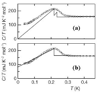
Figure 7: The specific heat coefficient of URhGe as observed in Ref. Aoki et al., 2001 (circles). The solid line in (a) shows the qualitative theoretical prediction for a perfect sample based on the present analysis. The one in (b) would apply if the down-spin electrons remained unpaired to the lowest observable temperature. The size of the discontinuity is known theoretically only in the weak-coupling limit;Vollhardt and Wölfle (1990) for the purpose of this qualitative illustration we have adjusted it to fit the maximum in the data.

V Discussion and conclusion

Let us further discuss several aspects of our theory and its implications. First, we consider in more detail our results regarding the magnetic susceptibility. In a normal conducting ferromagnetic phase, the transverse spin susceptibility is soft, displaying ferromagnetic magnons with a quadratic dispersion relation. The scale in the dispersion relation is set by the Stoner gap or exchange splitting $\delta$, which is proportional to the magnetization. In natural units, measuring wave numbers in units of the magnetic coherence length $\xi_{m}$, which is on the order of the Fermi wave number $k_{\text{F}}$, we have

$$\Omega\sim\delta\ ({\bf k}\xi_{m})^{2}\quad.$$

At zero frequency, the dimensionless transverse magnetic susceptibility diverges for ${\bm{k}}\to 0$ like

$$\chi_{\text{T}}({\bm{k}})=c/({\bm{k}}\xi_{m})^{2}\quad.$$

For a given distance from the magnetic phase transition, $c$ is a number of order one whose exact value depends on the details of the model. The Gaussian approximation we have employed correctly reflects these exact features, see Eqs. (26). In the presence of an up-spin gap, the structure of the magnon changes qualitatively. The Gaussian approximation for $\chi_{\text{T}}$ predicts a true gap, Eqs. (30). This is a consequence of the fact that the Gaussian approximation effectively treats the superconducting gap as a fixed external field. The LGW theory of Appendix A shows that this does not correctly reflect the symmetry properties of the system, and that the static $\chi_{\text{T}}$ actually has the structure

$$\chi_{\text{T}}({\bm{k}})=\frac{c}{({\bm{k}}\xi_{m})^{2}}\ \cfrac{1}{1+g\,\cfrac{2N_{\text{F}}\Gamma_{\text{t}}|\Delta_{\uparrow}|^{2}/\delta^{2}}{({\bm{k}}\xi_{m})^{2}+g\,(\xi_{m}/\xi_{\Delta})^{2}}}\quad.$$ (37a)

Here $$g {\tilde{g}} {\tilde{m}} g={\tilde{g}}\,{\tilde{m}} \chi_{\text{T}} {\bm{k}}^{2}<g\,\xi_{\Delta}^{-2} g \chi_{\text{T}}$$ is related to the coupling constant and the magnetic order parameter of the LGW theory by . This result shows that, in general, has a much more complicated structure than in the absence of spin-triplet superconductivity. At asymptotically small wave numbers, , drops out of the expression for , and we have

$$\chi_{\text{T}}({\bm{k}})=\frac{c}{{\bm{k}}^{2}}\ \frac{1}{1+(\Delta_{\uparrow}/\delta)^{2}\,(\xi_{\Delta}/\xi_{m})^{2}}\quad.$$ (37b)

Restoring the frequency, the dispersion relation of the magnon then is

$$\Omega\sim\delta\,\left[1+(\Delta_{\uparrow}/\delta)^{2}\,(\xi_{\Delta}/\xi_{m})^{2}\right]\,{\bm{k}}^{2}\quad.$$

We see that the magnon dispersion relation is substantially changed by the presence of $\Delta_{\uparrow}$ as long as the condition expressed by Eq. (48) is fulfilled. Namely, the magnon is much stiffer, i.e., the frequency rises much faster with the wave number, than in a normal conducting ferromagnet. The magnitude of this effect will depend on the detailed parameters of the material in question, but it clearly can be substantial: Assuming a value of $\Delta_{\uparrow}$ on the order of the superconducting $T_{\text{c}}$, or $\Delta_{\uparrow}\approx 1\text{K}$, a value of $\delta$ on the order of 10 times the magnetic $T_{\text{c}}$,del or $\delta\approx 100\text{K}$, and $\xi_{\Delta}/\xi_{m}\approx 1,000$, we find that the prefactor in the dispersion relation is enhance by a factor of 100 over its value in the normal conducting phase.

For larger wave numbers, ${\bm{k}}^{2}>g\,\xi_{\Delta}^{-2}$, we have

$$\chi_{\text{T}}({\bm{k}})\approx\frac{c}{({\bm{k}}\xi_{m})^{2}+g\,2N_{\text{F}}\Gamma_{\text{t}}\,|\Delta_{\uparrow}|^{2}/\delta^{2}}\quad.$$ (37c)

Using Eqs. (47), we have the correspondence $g\cong g(\delta/2T)/3\gtrsim 1$, so we recover the result of the Gaussian theory, Eqs. (30). As long as Eq. (48) is valid, $\chi_{\text{T}}$ thus displays a pronounced plateau as a function of the wave number, followed by a very steep increase at asymptotically small wave numbers. The Gaussian theory approximates this behavior by a true gap, ignoring the asymptotic regime. In the limit $\xi_{\Delta}/\xi_{m}\to\infty$ the asymptotic regime shrinks to zero, and the Gaussian theory becomes qualitatively correct. However, in this context one should note that the LGW theory of Appendix A is valid only for wave numbers $|{\bm{k}}|<\xi_{\Delta}^{-1}$. Within the LGW theory, the shoulder will lie in that regime provided the coupling constant ${\tilde{g}}$ is sufficiently small. While the above identification of ${\tilde{g}}$ with the parameters of the microscopic theory makes ${\tilde{g}}$ effectively of order unity, given the initial sharp rise of the magnon frequency with the wave number in the regime where the LGW is valid, a pronounced shoulder in the dispersion relation at intermediate wave numbers is inevitable. The wave number region where one expects this shoulder is given by

$$g\,\xi_{\Delta}^{-2}<{\bm{k}}^{2}<g\,(|\Delta_{\uparrow}|/\delta)^{2}\,\xi_{m}^{-2}\quad.$$ (38)

If we use the same numbers as above, and $g=1$, $\xi_{m}=1$Å, the upper limit of this wave-number range is given by $|{\bm{k}}|=0.01$Å. This is a factor of 3 below the smallest wave numbers currently observable with neutron scattering.Kittel (1996) However, in materials with smaller values of the exchange splitting $\delta$ the plateau should be in an observable regime.

Second, we add some comments about our prediction of two superconducting transitions that are separated only by a small temperature interval. Within our model, we have found this prediction to be very robust, especially given that all of our approximations have a tendency to overestimate the suppression of $T_{\text{c}\downarrow}$ compared to $T_{\text{c}\uparrow}$. Even an (artificial) increase of the gap in the transverse susceptibility by a factor of 10 does not make a visible change in Fig. 6. This reflects the fact that the up-spin and down-spin pairing are mediated by the same effective potential, viz., $\chi_{\text{L}}$, see Eq. (LABEL:eq:4.4a) and the corresponding Eq. (3.14a) in I. While $\chi_{\text{L}}$ is modified by $\Delta_{\uparrow}$, the effect is not sufficiently large to lead to a substantial separation of $T_{\text{c}\uparrow}$ and $T_{\text{c}\downarrow}$. This in turn means that the lower value of $T_{\text{c}\downarrow}$ is overwhelmingly due to the lower value of the density of states at the down-spin Fermi level. In this context we need to keep in mind that we have used a free-electron model with parabolic bands. A complicated band structure could lead to a drastically reduced value of $N_{\text{F}\downarrow}$, which in turn would lead to a much lower value of $T_{\text{c}\downarrow}$. If experiments on samples of improved quality should fail to show two transitions, this would be the most likely explanation. This would be of interest also with regard to distinguishing between the two proposed explanations for why the superconductivity is observed in the ferromagnetic phase only: Sandeman et al.Sandeman et al. (2003) have proposed a mechanism based on an intricate structure of the density of states, while the explanation proposed in I is based on properties of the magnetic susceptibility.

Third, we come back to our discussion of the specific heat. The experiment of Ref. Aoki et al., 2001 shows that the observed superconductivity is indeed a bulk effect. What is not clear a priori is the origin of the large residual value of the specific heat coefficient. While the down-spin electrons remaining unpaired, as was suggested in Ref. Aoki et al., 2001, is a possibility, normal-conducting regions within the sample would have the same effect and would also lead to the observed smearing of the discontinuity in the specific heat. With increasing sample quality, the discontinuity should become sharper, and a crucial question will be whether the residual value drops correspondingly. Of course, the emergence of the predicted double feature from the narrowing peak will be the most direct test of our predictions regarding the specific heat. In this context it is interesting to note that such a split transition, with two closely spaced discontinuities in the specific heat, has been observed in UPt₃,Fisher et al. (1989); Hasselbach et al. (1989) but only after a long period of gradually increasing sample quality. (UPt₃ is not ferromagnetic, though, and the split transition has a physical origin that is very different from what we have discussed.) Even in the best samples that show the split transition, however, there is a substantial residual specific heat coefficient, the origin of which is not quite clear. In a ferromagnetic superconductor, one also has to keep in mind that the ground state will not be homogeneous, due to the formation of a spontaneous vortex state.Greenside et al. (1981); Ng and Varma (1997); Radzihovsky et al. (2001) Normal electrons in the vortex cores are a possible source of a residual specific heat coefficient. This effect has been neglected in the current theory and will be pursued in a future publication.

Fourth, we briefly comment on the fact that the mass, or pseudo-mass, induced in the transverse magnetic susceptibility by the superconductivity, is a singular function of the magnetization. This can be seen in Eqs. (30), and it also leads to the factor of $1/\delta$ in the relation between the phenomenological coupling constant ${\tilde{g}}$ in the LGW theory and the microscopic parameters, Eq. (47c). This behavior can be traced back to the behavior of the integral in Eq. (30c), and thus ultimately to the Green functions and the soft particle-hole excitations that are characteristic for itinerant electron systems. The singularity is therefore a result of a coupling between the particle-hole excitations and the magnetic and superconducting Goldstone modes. It is very similar in nature to, e.g., the anomalous magnetization dependence of the magnon stiffness in a normal conducting ferromagnetic phase that was discussed in Ref. Belitz et al., 1998.

In conclusion, we summarize our results. We have presented a consistent and self-contained theory for the coexistence of superconductivity and ferromagnetism in itinerant electron systems. We have presented a field-theoretic formulation of this problem that allows for the determination of both the magnetic and the superconducting equation of state in a systematic loop expansion. This method, which utilizes Ma’s procedure for generating equations of state, remedies some shortcomings of the earlier theory presented in I, which relied on a minimization of the free energy. The self-contained character of the theory is achieved by means of explicit expressions for the magnetic susceptibility, which is needed as input for the generalized Eliashberg equations. These expressions have been evaluated in ferromagnetic phases, both normal conducting and superconducting ones. This is a generalization of the theory for the magnetic susceptibility that was developed in I, and it explicitly takes into account the feedback effects that are characteristic for any purely electronic mechanism for superconductivity.

We have explicitly evaluated this theory to one-loop order, and for a model that allows for two components of the superconducting order parameter, one each for Cooper pairs consisting of up-spin electrons and down-spin electrons, respectively. The limitations of this one-loop approximation, which neglects superconducting fluctuations and uses a zero-loop expression for the magnetic susceptibility, have been discussed by means of a phenomenological LGW theory that complements our microscopic theory. We have found that, for generic parameter values, the two superconducting transitions that describe the pairing of up-spin and down-spin electrons, respectively, occur close to one another, with transition temperatures that typically differ by only on the order of 10%. This suggests that, if the superconductivity observed in URhGe is indeed of a spin-triplet p-wave type mediated by ferromagnetic fluctuations, then the broad feature observed in the specific heat near the temperature of the resistive transitionAoki et al. (2001) should contain two transitions that are close together. If samples of improved quality should show only one sharp discontinuity in the specific heat, then this would be a strong argument against the type of pairing we have assumed in this paper. A caveat is provided by our assumption of parabolic bands, however, as discussed above. The presence of spin-triplet superconductivity has further been shown to drastically change the structure of the dispersion relation of the ferromagnetic magnons. In materials with a small exchange splitting this effect is observable with neutron scattering, and can also be used as a probe for the nature of the superconductivity.

Appendix A LGW theory

In this appendix we discuss the mean-field action $\mathcal{A}^{(0)}$, Eq. (8), or the corresponding Landau free energy density $f^{(0)}=-(T/V)\mathcal{A}^{(0)}$, and its generalization to a phenomenological LGW theory.

A.1 Landau theory

From Eq. (8) we have

$$f^{(0)}=\frac{\Gamma_{\text{t}}}{2}\,m^{2}-\frac{T}{V}\,{\text{Tr}}\,(\lambda\langle\mathcal{G}\rangle)-\frac{T}{2V}\,{\text{Tr}}\,\ln\tilde{G}^{-1}\quad.$$ (39)

In what follows we neglect the normal self-energy contribution to the matrix $\lambda$, Eqs. (6), which lead only to a trivial renormalization of the normal Green function. An expansion in powers of the order parameters $m$ and $\lambda$ then yields

$$f^{(0)} = {\text{Tr}}\,\left(\lambda^{\text{T}}(\langle\mathcal{G}^{\text{T}}\rangle-\tilde{G}_{0}/2)\right)-\frac{T}{4V}\,{\text{Tr}}\,\left(\lambda^{\text{T}}\tilde{G}_{0}\right)^{2}$$ (40)

$$\hskip-40.0pt+\frac{\Gamma_{\text{t}}}{2}\,t\,m^{2}-\frac{T\Gamma_{\text{t}}}{2V}\,m\,{\text{Tr}}\,\left(\tilde{G}_{0}\,\gamma_{3}\,\tilde{G}_{0}\lambda^{\text{T}}\,\tilde{G}_{0}\lambda^{\text{T}}\right)+\ldots$$

Here $t=1-2N_{\text{F}}\Gamma_{\text{t}}$ is the mean-field distance from the magnetic critical point, and we have omitted cubic terms of order $m^{3}$, $m^{2}\lambda$, and $\lambda^{3}$, as well as all quartic terms.

This mean-field free energy does not describe a superconducting transition; this requires magnetic loops, as we have seen in the main text. The magnetic part, however, agrees with an expansion of the mean-field magnetic equation of state, Eq. (14). In particular, the cubic term of $O(m\lambda^{2})$ shown in Eq. (40) has important consequences. For a nonzero superconducting order parameter $\Delta_{\uparrow}$, Eq. (6), the quantity

$$h_{\text{eff}}=\frac{T\Gamma_{\text{t}}}{2V}\,{\text{Tr}}\,\left(\tilde{G}_{0}\,\gamma_{3}\,\tilde{G}_{0}\lambda^{\text{T}}\,\tilde{G}_{0}\lambda^{\text{T}}\right)$$ (41a)

acts like an effective external magnetic field. Performing the trace, we have

$$h_{\text{eff}}=-\Gamma_{\text{t}}\,\frac{T}{V}\sum_{k}|\Delta_{\uparrow}(k)|^{2}\,|\tilde{G}_{0}(k)|^{2}\,\tilde{G}_{0}(k)\quad.$$ (41b)

General argumentsMa (1976) show that such a term in the free energy leads to a mass in the magnetic Goldstone mode, i.e., in the transverse spin susceptibility,

$$\chi_{\text{s}}^{-1}(k=0)=h_{\text{eff}}/m\quad.$$ (42)

If we expand Eq. (29) in powers of $\Delta_{\uparrow}$ and $m$, we see that this is indeed the same result we obtained in Sec. III by a direct calculation of the susceptibility. The current derivation makes it obvious that this result has been obtained while neglecting fluctuations. We consider the influence of fluctuations in the next subsection.

A.2 LGW theory

The conclusion in the previous subsection, namely, that the transverse spin susceptibility is massive, cannot be strictly correct. Even in the presence of superconducting order, one expects the system to be invariant under rotations of all spins, and this symmetry must manifests itself via a Goldstone mode to which the magnetic susceptibility must couple. To investigate this point, we consider the following phenomenological action,qua

$$S[{\bm{m}},{\bm{\phi}}] = \int d{\bm{x}}\ \left[t_{m}\,{\bm{m}}^{2}({\bm{x}})+\xi_{m}^{2}\,\left(\nabla{\bm{m}}({\bm{x}})\right)^{2}+u_{m}\,{\bm{m}}^{4}({\bm{x}})\right]+\int d{\bm{x}}\ \left[t_{\Delta}\,|{\bm{\phi}}({\bm{x}})|^{2}+\xi_{\Delta}^{2}\,|\nabla{\bm{\phi}}({\bm{x}})|^{2}+u_{\Delta}\,|{\bm{\phi}}({\bm{x}})|^{4}\right]$$ (43)

$$-i{\tilde{g}}\int d{\bm{x}}\ {\bm{m}}({\bm{x}})\cdot\left({\bm{\phi}}({\bm{x}})\times{\bm{\phi}}^{*}({\bm{x}})\right)\quad.$$

Here ${\bm{m}}$ and ${\bm{\phi}}$ are the magnetic and the superconducting order parameter, respectively, and the latter has been represented as a complex 3-vector in spin space.Vollhardt and Wölfle (1990) $t_{m}$ and $t_{\Delta}$ are the dimensionless distances from the magnetic and superconducting critical point, and $\xi_{m}$ and $\xi_{\Delta}$ are the (zero-temperature) magnetic and superconducting coherence lengths, respectively. ${\tilde{g}}$ is a phenomenological coupling constant. At the mean-field level, ${\bm{m}}=(0,0,{\tilde{m}})$, and ${\bm{\phi}}=({\tilde{\Delta}},i{\tilde{\Delta}},0)$, with ${\tilde{m}}\propto m$ and ${\tilde{\Delta}}\propto\Delta_{\uparrow}$, and the theory is seen to have the structure of the Landau theory derived from the miscroscopic theory in Sec. A.1 above.

This action is invariant under a symmetry group SO(3)$\times$U(1), which represents co-rotations of the vectors ${\bm{m}}$ and ${\bm{\phi}}$, and in addition a gauge transformation of the complex field ${\bm{\phi}}$. In the ordered state given above, this symmetry is spontaneously broken, and the ordered state is invariant only under rotations about the 3-axis. We thus expect dim(SO(3)$\times$U(1)/SO(2)) = 3 Goldstone modes. An explicit calculation, involving an expansion to Gaussian order about the ordered state, confirms this expectation. Of the three soft modes, two are spin wave-like modes, namely, superpositions of the transverse components of ${\bm{m}}$ and the 3-component of ${\bm{\phi}}$, while the third is an Anderson-Bogoliubov-like mode that reflects the broken gauge symmetry. Specifically, the transverse ${\bm{m}}$-susceptibility has an overlap with one of the spin-wave Goldstone modes. The Gaussian theory yields

$${\tilde{\chi}}_{\text{T}}({\bm{p}}) \equiv \langle m_{1}({\bm{p}})\,m_{1}(-{\bm{p}})\rangle$$ (44)

$$= \frac{{\tilde{m}}\xi_{m}^{-2}\,\left({\tilde{g}}{\tilde{m}}\xi_{\Delta}^{-2}+{\bm{p}}^{2}\right)}{2{\bm{p}}^{2}\,\left[{\tilde{g}}\left({\tilde{\Delta}}^{2}\xi_{m}^{-2}+{\tilde{m}}^{2}\xi_{\Delta}^{-2}\right)+{\tilde{m}}{\bm{p}}^{2}\right]}$$

From this result we see that, in the momentum range

$${\tilde{g}}\,{\tilde{m}}\,\xi_{\Delta}^{-2}<{\bm{p}}^{2}<{\tilde{g}}\,({\tilde{\Delta}}^{2}/{\tilde{m}})\,\xi_{m}^{-2}\quad,$$ (45)

the transverse susceptibility is effectively massive,

$${\tilde{\chi}}_{\text{T}}({\bm{p}})\approx{\tilde{m}}/2{\tilde{g}}{\tilde{\Delta}}^{2}\quad.$$ (46)

${\tilde{m}}$ and ${\tilde{\Delta}}$ can be related to $m$ and $\Delta_{\uparrow}$, respectively, in the microscopic theory by comparing Eq. (43) with the Landau theory in Sec. A.1 above. One finds the correspondence

$${\tilde{m}}\cong m\,\sqrt{\Gamma_{t}/2T}\quad,$$ (47a)

$${\tilde{\Delta}}\cong\Delta_{\uparrow}\,\sqrt{N_{\text{F}}/T}\quad.$$ (47b)

$${\tilde{g}} m \delta=\Gamma_{\text{t}}\,m g(\delta/2T)$$ does not corresponds to a simple constant in the microscopic theory, but rather to a function of (or ) and the function in Eq. (30c),

$${\tilde{g}}\cong\sqrt{2T\Gamma_{\text{t}}}\ \frac{1}{3\delta}\ g(\delta/2T)\quad.$$ (47c)

This complicated behavior of the effective coupling between the magnetic and superconducting order parameters is not reflected by the LGW theory. It is a result of the itinerant nature of the electrons, and the corresponding soft particle-hole excitations, as is discussed in Sec. V. Upon substituting Eqs. (47) in Eq. (46) we see that the latter is the same result as Eq. (30a) for the magnetic susceptibility.

The momentum range given by Eq. (45) exists only if the condition $\Delta\gg{\tilde{m}}\xi_{m}/\xi_{\Delta}$ is fulfilled. In terms of the Stoner gap $\delta=\Gamma_{\text{t}}\,m$ and $\Delta_{\uparrow}$ this condition takes the form

$$\delta/\Delta_{\uparrow}\ll\xi_{\Delta}/\xi_{m}\quad.$$ (48)

These results are further discussed in Sec. V.

Appendix B The spin susceptibility

In this appendix we establish the relation between the physical spin susceptibility $\chi_{\text{s}}$, as measured, e.g., by neutron scattering, and the quantity $\chi$ that emerges as the $\delta\bm{M}$ propagator of our field theory, see Eqs. (9, 10). We start by adding a magnetic field $\bm{h}(x)$ to our action that couples linearly to the electron spin density and acts as a source field for spin-density correlation functions. The action, Eq. (1), becomes

$${\cal A}[{\bm{M}},{\cal G},\Lambda;\bm{h}] = {\text{Tr}}\,(\Lambda{\cal G})-\int dx\ {\bm{M}}(x)\cdot{\bm{M}}(x)$$ (49)

$$\hskip-75.0pt+\frac{1}{2}{\text{Tr}}\,\ln({\tilde{G}}_{0}^{-1}+\sqrt{2\Gamma_{\text{t}}}{\bm{\gamma}}\cdot{\bm{M}}-\Lambda^{\text{T}}+\bm{\gamma}\cdot\bm{h})\quad.$$

The partition function,

$$Z[\bm{h}]=\int D[\delta\bm{M},\delta\lambda,\delta\mathcal{G}]\ e^{{\cal A}[{\bm{M}},{\cal G},\Lambda;\bm{h}]}\quad,$$ (50)

then serves as the generating functional for the magnetization,

$$m=\langle n_{\text{s}}^{3}(x)\rangle=\frac{\delta}{\delta h_{3}(x)}\Biggl{|}_{\bm{h}=0}\ \ln Z[h]\quad,$$ (51)

and for the spin susceptibility,

$$\chi_{\text{s}}^{ij}(x-y)=\langle\delta n_{\text{s}}^{i}(x)\,\delta n_{\text{s}}^{j}(y)\rangle=\frac{\delta^{2}}{\delta h_{i}(x)\,\delta h_{j}(y)}\Biggl{|}_{\bm{h}=0}\ \hskip-5.0pt\ln Z[h]\ ,$$ (52)

where $\bm{n}_{\text{s}}(x)$ is the electron spin density, and $\delta n_{\text{s}}^{i}(x)=n_{\text{s}}^{i}(x)-\langle n_{\text{s}}^{i}(x)\rangle$.

The simplest way to deal with the source field is to shift $\bm{M}$: $\bm{M}(x)\rightarrow\bm{M}(x)-\bm{h}(x)/\sqrt{2\Gamma_{\text{t}}}$. We then find

$$m=\sqrt{2/\Gamma_{\text{t}}}\,\langle M_{3}(x)\rangle\quad,$$ (53)

in agreement with Eq. (5a). An evaluation of $\langle M_{3}(x)\rangle$ to one-loop order yields the magnetic equation of state, Eq. (14). Similarly,

$$\chi_{\text{s}}^{ij}(x-y)=\langle\delta M_{i}(x)\,\delta M_{j}(y)\rangle-\delta_{ij}\,\delta(x-y)\quad.$$ (54)

If we evaluate the $\delta\bm{M}$-correlation function in Gaussian approximation, we findshi

$$\chi_{\text{s}}^{ij}(x-y)\approx\left[\chi_{ij}(x-y)-\delta_{ij}\,\delta(x-y)\right]/\Gamma_{\text{t}}\quad.$$ (55)

We see that the $\delta\bm{M}$-propagator of the field theory is simply related to the physical spin susceptibility. In particular, the transverse part of $\chi_{\text{s}}$ is massive if and only if that of $\chi$ is. For the Fourier transform of the longitudinal part, we find from Eq. (55)

$$\chi_{\text{s}}^{\text{L}}(k)\equiv\chi_{\text{s}}^{33}(k)=\frac{-\chi_{\text{L}}^{0}(k)}{1+\Gamma_{\text{t}}\chi_{\text{L}}^{0}(k)}\quad,$$ (56)

which has the expected RPA-type structure. Notice that the “contact term”, which results from the term in $\mathcal{A}$ that is quadratic in $\bm{h}$, provides the numerator in Eq. (56) that is missing in $\chi_{\text{L}}$.

References

- Saxena et al. (2000) S. S. Saxena, P. Agarwal, K. Ahilan, F. M. Grosche, R. K. W. Haselwimmer, M. J. Steiner, E. Pugh, I. R. Walker, S. R. Julian, P. Monthoux, et al., Nature 406, 587 (2000).
- Huxley et al. (2001) A. Huxley, I. Sheikin, E. Ressouche, N. Kernavanois, D. Braithwaite, R. Calemczuk, and J. Flouquet, Phys. Rev. B 63, 144519 (2001).
- Aoki et al. (2001) D. Aoki, A. Huxley, E. Ressouche, D. Braithwaite, J. Floquet, J. P. Brison, E. Lhotel, and C. Paulsen, Nature 413, 613 (2001).
- Pfleiderer et al. (2001) C. Pfleiderer, M. Uhlarz, S. M. Hayden, R. Vollmer, H. von Löhneysen, N. R. Bernhoeft, and G. G. Lonzarich, Nature 412, 58 (2001).
- (5) Spin-triplet superconductivity induced by magnetic fluctuations was predicted to occur in ZrZn2 as early as 1980 by Fay and Appel, Ref. Fay and Appel, 1980. Band structure calculations for UGe2, Ref. Shick and Pickett, 2001, and ZrZn2, Ref. Santi et al., 2001, have concluded that this mechanism is indeed a possibility in these materials. Other mechanisms have been proposed in Refs. Shimahara and Kohmoto, 2002; Blagoev et al., 1999; Watanabe and Miyake, 2002. Ref. Sandeman et al., 2003 has proposed that a density-of-states effect is responsible for the asymmetry of the phase diagram in UGe2, independent of the nature of the pairing interaction.
- Fay and Appel (1980) D. Fay and J. Appel, Phys. Rev. B 22, 3173 (1980).
- Kirkpatrick and Belitz (2003) T. R. Kirkpatrick and D. Belitz, Phys. Rev. B 67, 024515 (2003), see also T. R. Kirkpatrick, D. Belitz, T. Vojta, and R. Narayanan, Phys. Rev. Lett. 87, 127003 (2001).
- Tateiwa et al. (2001) N. Tateiwa, T. C. Kobayashi, K. Hanazono, K. Amaya, Y. Haga, R. Settai, and Y. Onuki, J. Phys.: Cond. Matter 13, L17 (2001).
- Vollhardt and Wölfle (1990) D. Vollhardt and P. Wölfle, The Superfluid Phases of Helium 3 (Taylor & Francis, 1990).
- (10) In addition, the superconducting state cannot be uniform, but must display a spontaneous flux-lattice structure, with both the magnetic and the superconducting order parameters showing spatial modulation. We will ignore this effect in this paper and come back to it in a separate publication.
- (11) T. R. Kirkpatrick and D. Belitz, eprint cond-mat/0307348, to appear in Phys. Rev. Lett.
- (12) While the end result in I was correct, the derivation contained a number of compensating errors.
- Ma (1976) S.-K. Ma, Modern Theory of Critical Phenomena (Benjamin, Reading, MA, 1976).
- (14) This is closely related to the diagram rules in Sec. IV.A of Ref. Belitz and Kirkpatrick, 1997.
- (15) Equation (3.10) in I had a factor of missing.
- (16) It is not obvious what the free energy should be minimized with respect to, and what should be kept constant in such a procedure. While the end result in I was correct, the derivation contained a number of compensating errors. This is the main reason why Ma’s method is advantageous compared to a minimization of the free energy.
- Forster (1975) D. Forster, Hydrodynamic Fluctuations, Broken Symmetry, and Correlation Functions (Benjamin, Reading, MA, 1975).
- Pao and Bickers (1991) C.-H. Pao and N. E. Bickers, Phys. Rev. B 44, 10270 (1991).
- Brinkman and Engelsberg (1968) W. F. Brinkman and S. Engelsberg, Phys. Rev. 169, 417 (1968).
- Brézin and Wallace (1973) E. Brézin and D. J. Wallace, Phys. Rev. B 7, 1967 (1973).
- Belitz et al. (1989) D. Belitz, S. D. Souza-Machado, T. P. Devereaux, and D. W. Hoard, Phys. Rev. B 39, 2072 (1989).
- (22) This assumes that the transition is of second order. Close to the ferromagnetic quantum critical point, this may not be the case, see Ref. Chubukov et al., 2003.
- (23) The code used to calculate in zero-loop approximation in I had the wave number in pinned to the paramagnetic Fermi surface rather than to the up-spin Fermi surface. As a consequence, our present results for differ slightly from those in I for the same parameter values.
- (24) In the elemental ferromagnets Fe and Co the exchange splitting is larger than the Curie temperature by a factor on the order of 10.Kübler (2000) For the superconducting ferromagnets of interest here we are not aware of any values for .
- Kittel (1996) C. Kittel, Introduction to Solid State Physics (Wiley, New York, 1996).
- Sandeman et al. (2003) K. Sandeman, G. Lonzarich, and A. Schofield, Phys. Rev. Lett. 90, 167005 (2003).
- Fisher et al. (1989) R. A. Fisher, S. Kim, B. F. Woodfield, N. E. Phillips, L. Taillefer, K. Hasselbach, J. Flouquet, A. L. Georgi, and J. L. Smith, Phys. Rev. Lett. 62, 1411 (1989).
- Hasselbach et al. (1989) K. Hasselbach, L. Taillefer, and J. Flouquet, Phys. Rev. Lett. 63, 93 (1989).
- Greenside et al. (1981) H. S. Greenside, E. I. Blount, and C. M. Varma, Phys. Rev. Lett. 46, 49 (1981).
- Ng and Varma (1997) T. K. Ng and C. M. Varma, Phys. Rev. Lett. 78, 330 (1997).
- Radzihovsky et al. (2001) L. Radzihovsky, E. M. Ettouhami, K. Saunders, and J. Toner, Phys. Rev. Lett. 87, 027001 (2001).
- Belitz et al. (1998) D. Belitz, T. R. Kirkpatrick, A. J. Millis, and T. Vojta, Phys. Rev. B 58, 14155 (1998).
- (33) In addition to the quartic term , there is in general also a term . Adding this term does not change our conclusions.
- (34) Note that this relation holds both before and after the shifts that diagonalize the Gaussian action. The reason is the same cancellation that leads to the diagram rule in Sec. II.3.
- Shick and Pickett (2001) A. Shick and W. Pickett, Phys. Rev. Lett. 86, 300 (2001).
- Santi et al. (2001) G. Santi, S. B. Dugdale, and T. Jarlborg, Phys. Rev. Lett. 87, 247004 (2001).
- Shimahara and Kohmoto (2002) H. Shimahara and M. Kohmoto, Europhys. Lett. 57, 247 (2002).
- Blagoev et al. (1999) K. B. Blagoev, J. R. Engelbrecht, and K. S. Bedell, Phys. Rev. Lett. 82, 133 (1999).
- Watanabe and Miyake (2002) S. Watanabe and K. Miyake, J. Phys. Soc. Jpn. 71, 2489 (2002).
- Belitz and Kirkpatrick (1997) D. Belitz and T. R. Kirkpatrick, Phys. Rev. B 56, 6513 (1997).
- Chubukov et al. (2003) A. V. Chubukov, A. M. Finkelstein, R. Haslinger, and D. K. Morr, Phys. Rev. Lett. 90, 077002 (2003).
- Kübler (2000) J. Kübler, Theory of Itinerant Electron Magnetism (Clarendon Press, Oxford, 2000).