First-order superfluid-Mott insulator transition of spinor bosons in an optical lattice

Abstract

We study the superfluid-Mott insulator transition of antiferromagnetic spin-1 bosons in an optical lattice described by a Bose-Hubbard model. Our variational study with the Gutzwiller-type trial wave function determines that the superfluid-Mott insulator transition is a first-order one at a part of the phase boundary curve, contrary to the spinless case. This first-order transition may be observed through an experiment, such as a Stern-Gerlach type, under a magnetic field.

Superfluid (SF) transition is one of the most striking phenomena of condensed matter physics. In particular, critical phenomena of superfluid transition, including the order of the transition, have been extensively studied for several decades. The quantum superfluid-Mott insulator (SF-MI) transition has been studied in granular superconductors Goldman , Josephson-junction arrays Fazio , and helium absorbed in the porous media Reppy . Recently, the SF-MI transition of bosons in an optical lattice has been very clearly observed Greiner . Jaksch et al. Jaksch have shown that bosons in an optical lattice can be described by a Hubbard model M.P.A.Fisher (a Bose-Hubbard model). The Bose-Hubbard model for spinless bosons has been theoretically studied for the last two decades M.P.A.Fisher ; QMC ; BoseGutz ; Oosten ; Sheshadri . Monte Carlo studies QMC have confirmed that the transitions of the clean and dirty Bose-Hubbard models of spinless bosons are continuous as suggested by analytical studies M.P.A.Fisher .

It is also interesting to study the Bose-Hubbard model of spinor bosons spinor . Demler and Zhou DemlerZhou have discussed several unique properties of spin-1 bosons in an optical lattice. In a previous paper Tsuchiya , we determined the SF-MI phase boundary of spin-1 bosons with an antiferromagnetic interaction using a perturbative mean-field approximation (PMFA) Oosten , which gives a phase boundary close to that obtained by Monte Carlo studies for the case of spinless bosons.

An excellent trial wave function for studying the Bose-Hubbard model is a Gutzwiller-type wave function (GW) Gutzwiller , which has been frequently used for the Hubbard model for electrons Yokoyama . For spinless bosons, the GW describes a second-order SF-MI transition and obtains a phase boundary curve, which is in an exact agreement with that obtained using the PMFA Oosten . A GW for spinor bosons has been employed only recently for a non-uniform system Yamashita .

In the present study, by employing the GW, we show the SF-MI transition can be a first-order one at a part of the phase boundary. The first-order SF-non-SF transition is rare and interesting. For example, as stated above, the SF-MI transition of the spinless bosons is second-order one M.P.A.Fisher . Hence, the spin degree of freedom has an essential role in the first-order transition. The first-order transition can be observed by experiments, such as Stern-Gerlach type, under a magnetic field.

The Bose-Hubbard Hamiltonian DemlerZhou ; nematic1 ; note1 of spin-1 bosons is given by $H=H_{0}+H_{1}$,

$$H_{0} = -t\sum_{\langle i,j\rangle}\sum_{\alpha}(a_{i\alpha}^{\dagger}a_{j\alpha}+a_{j\alpha}^{\dagger}a_{i\alpha}),$$

$$H_{1} = -\mu\sum_{i}\sum_{\alpha}a_{i\alpha}^{\dagger}a_{i\alpha}+\frac{1}{2}U_{0}\sum_{i}\sum_{\alpha,\beta}a_{i\alpha}^{\dagger}a_{i\beta}^{\dagger}a_{i\beta}a_{i\alpha}$$ (1)

$$+\frac{1}{2}U_{2}\sum_{i}\sum_{\alpha,\beta,\gamma,\delta}a_{i\alpha}^{\dagger}a_{i\gamma}^{\dagger}{\bf F}_{\alpha\beta}\cdot{\bf F}_{\gamma\delta}a_{i\delta}a_{i\beta}.$$

$$= \sum_{i}[-\mu\hat{n}_{i}+\frac{1}{2}U_{0}\hat{n}_{i}(\hat{n}_{i}-1)+\frac{1}{2}U_{2}({\hat{\mathbf{S}}_{i}}^{2}-2\hat{n}_{i})].$$

Here, $\mu$ and $t$ are the chemical potential and the hopping matrix element between adjacent sites, respectively. $U_{0}$ and $U_{2}$ represent the spin-independent and the spin-dependent interactions between bosons, respectively. We assume an antiferromagnetic interaction ($U_{2}>0$). $a_{i\alpha}$ and $a_{i\alpha}^{\dagger}$ are the annihilation and creation operators, respectively, for a boson at site $i$ with spin magnetic quantum number $\alpha=1,0,-1$. $n_{i}\equiv\sum_{\alpha}n_{i\alpha}$ ($n_{i\alpha}\equiv a_{i\alpha}^{\dagger}a_{i\alpha}$) is a number operator at site $i$. ${\hat{\bf S}_{i}}\equiv\sum_{\alpha,\beta}a_{i\alpha}^{\dagger}{\bf F}_{\alpha\beta}a_{i\beta}$ is a spin operator at site $i$ and ${\bf F}_{\alpha\beta}$ represent the spin-1 matrices. $\langle i,j\rangle$ expresses a summation for all the sets of adjacent sites.

The GW of the model is defined as $\Psi\equiv\prod_{i}\Phi_{i}$. Here, $\Phi_{i}$ is a wave function at site $i$ but the functional form of $\Phi_{i}$ is assumed to be site-independent such that $\Phi_{i}=\Phi$. $\Phi$ is written as a linear combination of states with $N$ bosons at a site as $\Phi=\sum_{N}g(N)|N\rangle$, where $|2n+1\rangle=\sum^{2n+1}_{S=1}f(2n+1,S)|2n+1,S\rangle$ and $|2n\rangle=\sum^{2n}_{S=0}f(2n,S)|2n,S\rangle$; $|N,S\rangle$ is the state where $N$ is the number of bosons and $S$ is the total spin, where $S$ must be odd for an odd and even for an even $N$ DemlerZhou . We assume that ${\hat{S}}_{z}|N,S\rangle=0$ note2 . Hence, $\Phi$ is an eigenstate of $S_{z}$ (not $S$) as a quantum spin nematic state nematic1 in the MI state. $\Phi$ can interpolate between two limits about $U_{2}$ as $\Phi=\sum_{n}[g(2n)|2n,S=0\rangle+g(2n+1)|2n+1,S=1\rangle]$ ($U_{2}\rightarrow\infty$) that minimizes the antiferromagnetic interaction $H_{\rm AF}\equiv\frac{1}{2}\sum_{i}U_{2}({\hat{\mathbf{S}}_{i}}^{2}-2\hat{n}_{i})$ and $\Phi=\sum_{n}g(N)a_{0}^{\dagger N}|0\rangle/\sqrt{N!}$ ($U_{2}\rightarrow 0$) that includes high-spin states and minimizes the kinetic energy, where $|0\rangle$ is the vacuum of bosons. We note that the latter GW for $U_{2}=0$ has the same form as the GW of the spinless bosons BoseGutz . We numerically optimize the variational parameters $g(N)$ and $f(N,S)$ to minimize the energy expectation value by Powell’s method numerical under the normalization conditions $\sum_{N}|g(N)|^{2}=1$ and $\sum_{S}|f(N,S)|^{2}=1$. We select the states where the number of bosons range from $N=0$ to $N=6$, which are sufficient for a numerical convergence in the parameter regime studied in this paper. We define that the MI phase has a zero particle number fluctuation, and the SF phase has a finite particle number fluctuation note0 . In an SF phase close to an MI one with $N$ bosons, probability densities of the states for a different values of $N$ can be considered as SF order parameters.

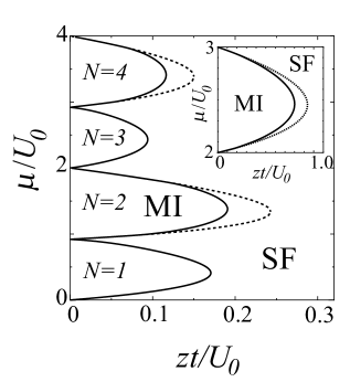
Figure 1: Phase diagram of the Bose-Hubbard model of spin-1 bosons for $U_{2}/U_{0}=0.04$. Here, $z$ is the number of adjacent sites in the lattice. SF and MI indicate the superfluid and the Mott-insulating phases, respectively. The solid and dashed curves are obtained using the GW and the PMFA, respectively. The inset indicates the SF-MI phase boundary around the MI state with $N=3$ for $U_{2}/U_{0}=0.001$.

Figure 1 shows the phase diagram for $U_{2}/U_{0}=0.04$, which corresponds to ${}^{23}{\mathrm{N}a}$ atoms spinor . The solid and dashed curves indicate the SF-MI phase boundaries using the GW and the PMFA, respectively. Here, $z$ is the number of adjacent sites in the lattice. Interestingly, at a part of the phase boundary curves, the GW slightly redefines the phase boundary curves obtained using the PMFA. It will be important to note that for spinless bosons, the phase boundary obtained using the GW is the same as that obtained using the PMFA. However, an even-odd conjecture predicted in Ref. Tsuchiya still clearly holds; the MI phase with an even $N$ is strongly stabilized against the SF phase.

On the other hand, in Fig. 1, the SF-MI phase boundary around the MI phase with an odd $N$ obtained using the GW is the same as that obtained using the PMFA. This agreement always holds around the MI phase with $N=1$. However, if we assume a much smaller $U_{2}$, we see a similar discrepancy between the two methods (inset of Fig. 1) around the MI phase with $N=3$.

It should be noted that the GW including only a set of low-spin states exactly reproduces the phase boundary obtained using the PMFA. For an even $N=2n$, assuming $g(2n\pm 1)=\epsilon_{2n\pm 1}$, $g(2n)=\sqrt{1-\epsilon_{2n+1}^{2}-\epsilon_{2n-1}^{2}}$, and $f(2n\pm 1,S=1)=f(2n,S=0)=1$ ($\epsilon_{2n\pm 1}$ are infinitesimal), we analytically reproduce the phase boundary curve around the Mott phase with $N=2n$ obtained using the PMFA (Eq. 30 in Ref. Tsuchiya ). We also reproduce the phase boundary obtained using the PMFA around the Mott phase with an odd $N=2n+1$ by numerical optimization of the GW only including the states $|2n+1,S=1\rangle$, $|2n+2,S=0\rangle$, $|2n+2,S=2\rangle$, $|2n,S=0\rangle$, and $|2n,S=2\rangle$. These sets of the low-spin states are nothing but the states that emerge as zero-order states or intermediate states in the second-order PMFA which determines the phase boundary Tsuchiya . This is consistent with the case of the phase boundary around the Mott state with $N=1$ and that of spinless bosons.

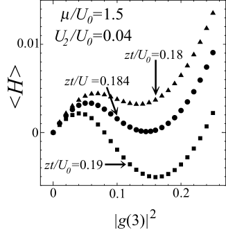
Figure 2: Expectation values of the total energy per site $\langle H\rangle$ as a function of $|g(3)|^{2}$ for $U_{2}/U_{0}=0.04$ and $\mu/U_{0}=1.5$. The other variational parameters are determined to minimize the energy. The origin of the vertical axis corresponds to the energy of the MI state with $N=2$. $zt=1.9$, $zt=1.84$, and $zt=1.8$ correspond to an MI state, a state very close to the phase boundary, and an SF state, respectively.

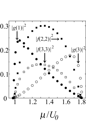
Figure 3: Variational parameters just on the phase boundary between the SF and MI phases with $N=2$ for $U_{2}/U_{0}=0.04$. The black and white circles indicate $|g(1)|^{2}$ and $|g(3)|^{2}$, respectively and the black and white squares indicate $|f(2,2)|^{2}$ and $|f(3,3)|^{2}$, respectively.

In our GW, the SF phase has a polar symmetry ($\langle{\bf S}\rangle=0$) and not only does the lowest spin state ($S=1$ or $S=0$) at a given $N$ but also higher spin states have finite probability densities. The probability densities of the high spin states and SF order parameters are finite just on a part of the phase boundary curve as long as the phase boundary curve does not agree with that obtained using the PMFA (hereafter, we call this part of the phase boundary curve as the non-perturbative part). Figure 2 shows the total energy expectation value par site $\langle H\rangle$ as a function of $|g(3)|$ around a MI phase with $N=2$, where we see the first-order transition clearly. The high spin states of spin-1 bosons have an essential role in the first-order transition: for small $|g(3)|$, the PMFA calculation holds and the total energy increases with $|g(3)|$; for large $|g(3)|$, $|f(2,2)|$ and $|f(3,3)|$ become large and strongly enhance the absolute value of the kinetic energy and the total energy decreases with $|g(3)|$; for much larger $|g(3)$, the interaction energy within $|N=3\rangle$ becomes larger and the total energy again increases with $|g(3)|$. In summation, the transition between the MI with only the lowest spin state (which has the lowest antiferromagnetic interaction energy) and the SF with higher spin states (which has a large absolute value of kinetic energy) can be a first-order one.

Figure 3 shows the chemical potential dependence of variational parameters including SF order parameters ($|g(1)|^{2}$ and $|g(3)|^{2}$) just on the phase boundary around the MI phase with $N=2$. These parameters are found to be finite on the non-perturbative part and continuously disappear at the edges of the non-perturbative part ($\mu/U_{0}\sim 0.97$ and $1.79$) where the phase boundary curve agrees with that obtained using the PMFA and the transition becomes a second-order one as in the spinless case.

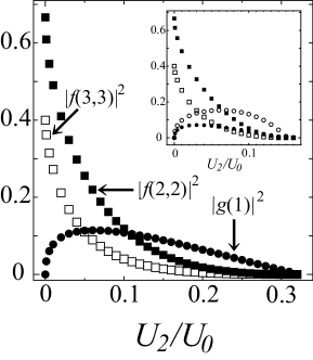
Figure 4: Variational parameters just on the Mott lobe of the phase boundary between the SF and MI phases with $N=2$ as a function of $U_{2}$. The black circles indicate $|g(1)|^{2}$, the black and white squares indicate $|f(2,2)|^{2}$ and $|f(3,3)|^{2}$, respectively. Here, $|g(3)|=|g(1)|$ within numerical errors. The inset indicates the same variational parameters including $|g(3)|^{2}$ (white circles) for $\mu=1.5/U_{0}$ just on the phase boundary.

The phase boundary curve obtained using the GW around the MI phase with $N$ bosons becomes close to that obtained using the PMFA for a stronger $U_{2}$ and coincide with it for a finite $U_{2}$ (e.g., $U_{2}/U_{0}\sim 0.32$ for $N=2$ and $U_{2}/U_{0}\sim 0.014$ for $N=3$), where the transition becomes a second-order one along the whole phase boundary. On the other hand, for $U_{2}=0$, the transition also becomes a second-order one because the GW has the same form as that of the spinless bosons [See above (the sixth paragraph)]. Figure 4 shows the variational parameters just on the Mott lobe of the phase boundary between the SF phase and the MI phase with $N=2$ as a function of $U_{2}/U_{0}$. Here, $\mu$ and $zt$ are determined as a function of $U_{2}$ to obtain the variational parameters just at the Mott lobe. We note that the Mott lobe stays on the non-perturbative part until the phase diagram perfectly coincides with that obtained using the PMFA for $U_{2}/U_{0}\sim 0.32$. Furthermore, $|g(3)|=|g(1)|$ holds within numerical errors. While SF order parameters $g(1)$ and $g(3)$ disappear for $U_{2}=0$ and $U_{2}/U_{0}\sim 0.32$, $|f(2,2)|^{2}$ and $|f(3,3)|^{2}$ become larger for small $U_{2}/U_{0}$ and attain the maximum values for $U_{2}/U_{0}=0$. This is because for $U_{2}/U_{0}=0$, $|N=2\rangle=a_{0}^{\dagger 2}|0\rangle/\sqrt{2!}=(|2,0\rangle+\sqrt{2}|2,2\rangle)/\sqrt{3}$ and $|N=3\rangle=a_{0}^{\dagger 3}|0\rangle/\sqrt{3!}=(\sqrt{3}|3,1\rangle+\sqrt{2}|3,3\rangle)/\sqrt{5}$, resulting in $|f(2,2)|^{2}=2/3$ and $|f(3,3)|^{2}=2/5$. The inset of Fig.4 shows the $U_{2}$ dependence of the variational parameters for $\mu/U_{0}=1.5$ just on the phase boundary between the SF and MI phases with $N=2$, where $zt$ is determined to obtain the variational parameters just at the phase boundary as a function of $U_{2}$. The SF order parameters (where $|g(3)|$ is different from $g(1)$) continuously disappear for $U_{2}/U_{0}\sim 0.15$, where $\mu/U_{0}=1.5$ on the phase boundary appears away from the non-perturbative part.

The first-order transition may be observed in future experiments. If the lifetimes of locally stable states are sufficiently long, one can observe the first-order transition through a hysteresis curve because $t/U_{0}$ and $t/U_{2}$ can be easily controlled by the laser beam. On the other hand, the first-order transition may also be observed through the response of a spin to a weak magnetic field. The magnetization (spin expectation value) under a magnetic field may be observed by an experiment such as a Stern-Gerlach type time-of-flight measurement as discussed in Ref. plateau . We consider a uniform magnetic field parallel to the $x$-axis note4 . We add the Zeeman coupling $-g\mu_{B}B\sum_{i}S_{xi}$ to the Hamiltonian, where $g$ is the Lande’s $g$-factor of bosons, $\mu_{B}$ is a Bohr magneton, $B$ is the magnetic field, and $S_{xi}$ is the $x$-component of the spin at site $i$. We neglect the quadratic Zeeman term because a weak magnetic field of the order of mGauss or less than mGauss is sufficient plateau . In the GW, the magnetization is also site-independent such that $\langle S_{xi}\rangle=\langle S_{x}\rangle$. In a magnetic field, the $S_{z}=0$ states are not sufficient to obtain the ground state, and hence, we employ the complete set with $S_{z}=-S,-S+1,\cdot\cdot\cdot,S$ in the GW. Figure 5 shows the $zt/U_{0}$ dependence of $\langle S_{x}\rangle$ for $U_{2}/U_{0}=0.04$ and $\mu/U_{0}=1.5$ under a magnetic field $g\mu_{B}B=0.005$ note6 . We can clearly see that $\langle S_{x}\rangle$ jumps from zero to a finite value for $zt/U_{0}\sim 1.85$, which corresponds to the SF-MI phase boundary under the magnetic field, and is close to that at zero magnetic field $zt/U_{0}\sim 1.84$. In the MI phase, the singlet state at a site is stable under a weak magnetic field, while in the SF phase, it has a finite spin at a site resulting in a finite $\langle S_{x}\rangle$ under a magnetic field.note7 However, if the transition is continuous, $\langle S_{x}\rangle$ must be a continuous function and should not jump at the phase boundary. Hence, this jump of $\langle S_{x}\rangle$ is a unique result of the first-order transition.

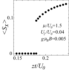
Figure 5: $zt/U_{0}$ dependence of $\langle S_{x}\rangle$ for $U_{2}/U_{0}=0.04$ and $\mu/U_{0}=1.5$ under a magnetic field $g\mu_{B}B=0.005$.

We finally note that recent studies nematic1 have predicted possible nematic phases in the MI phase, while our approximation results in the lowest spin state in the MI phase regardless of the strength of $U_{2}(>0)$; our study using the GW cannot include the effects of virtual hopping processes, which result in Heisenberg type spin-spin couplings between adjacent sites. However, the singlet-nematic phase boundary will be out of the MI phase in small densities of ${}^{23}{\mathrm{N}a}$ atoms such as two atoms per site (the case of which is well studied in the present paper) note5 . As a matter of course, the relation and/or competition between the SF-MI transition and the singlet-nematic transition will be an interesting and open subject.

We acknowledge M. Yamashita, M.W. Jack, T. Morishita, S. Watanabe, and K. Kuroki for helpful discussions. T. K. gratefully acknowledges financial support through a Grant-in-Aid for the 21st COE Program (Physics of Systems with Self-Organization Composed of Multi-Elements). S. T. is supported by the Japan Society for the Promotion of Science. A part of the numerical calculations was performed at the Supercomputer Center, Institute for Solid State Physics, University of Tokyo.

References

- (1) C.Christiansen, L. M. Hernandez, and A. M. Goldman, Phys. Rev. Lett. 88, 037004 (2002).
- (2) R. Fazio and H. van der Zant, Phys. Rep. 355, 235 (2001).
- (3) M.H.W. Chan, K.I. Blum, S.Q. Murphy, G.K.S. Wong, and J.D. Reppy, Phys. Rev. Lett. 61, 1950 (1988).
- (4) M. Greiner et al., Nature 415, 918 (2002).
- (5) D. Jaksch et al., Phys. Rev. Lett. 81, 3108 (1998).
- (6) M.P.A. Fisher, P.B. Weichman, G. Grinstein, and D.S. Fisher, Phys. Rev. B 40, 546 (1989).
- (7) G.G. Batrouni, R.T. Scalettar and G.T Zimanyi, Phys. Rev. Lett. 65, 1765 (1990); W. Krauth and N. Trivedi, Europhys. Lett. 14, 627 (1991).
- (8) D.S. Rokhsar and B.G. Kotliar, Phys. Rev. B 44, 10328 (1991); W. Krauth, M. Caffarel and J.-P. Bouchaud, Phys. Rev. B 45, 3137 (1992).
- (9) D. van Oosten, P. van der Straten, and H.T.C. Stoof, Phys. Rev. A 63, 053601 (2001).
- (10) K. Sheshadri, H. R. Krishnamurthy, R. Pandit, and T.V. Ramakrishnan, Europhys. Lett. 22, 257 (1993).
- (11) T.-L. Ho, Phys. Rev. Lett. 81, 742 (1998); T. Ohmi and K. Machida, J. Phys. Soc. Jpn. 76, 1822 (1998); D.M. Stamper-Kurn et al., Phys. Rev. Lett. 80, 2027 (1998).
- (12) E. Demler and F. Zhou, Phys. Rev. Lett. 88, 163001 (2002).
- (13) S. Tsuchiya, S. Kurihara, and T. Kimura, preprint (cond-mat/0209676).
- (14) M.C. Gutzwiller, Phys. Rev. 137, A1726 (1965).
- (15) See, e.g., H. Yokoyama and H. Shiba, J. Phys. Soc. Jpn. 57, 2482 (1988) and references therein.
- (16) M. Yamashita and M.W. Jack, preprint.
- (17) A. Imambekov, M. Lukin, and E. Demler, Phys. Rev. A 68, 063602 (2003); M. Snoek and F. Zhou, Phys. Rev. B 69, 094410 (2004).
- (18) For simplicity, we neglect the weak trapping potential and assume that the system is perfectly periodic.
- (19) We have numerically checked that the complete set including states with finite has the same lowest energy as that of the states with only at least within the states where the number of particles range from to .
- (20) A GW has a unique spin state in an MI because our approximation does not include inter-site effective spin coupling through virtual hopping processes nematic1 in the MI.
- (21) Strictly speaking, the nematic axis turns in a direction perpendicular to the magnetic field to minimize the Zeeman energy when a magnetic field is applied. [For further details, see F. Zhou, Int. J. Mod. Phys. B 17, 2643 (2003).]
- (22) In refs.nematic1 it is suggested that the singlet-nematic transition occurs for in the Mott state with two bosons, which corresponds to for in the case of three dimensional cubic lattices with (also see Fig. 1).
- (23) To obtain this figure, we have employed a complete set where the number of bosons range from to . The states with have very small amplitudes ( and ), and hence, the numerical convergence is fairly sufficient.
- (24) W.H. Press, S.A. Teukolsky, and W.T. Vetterling, Numerical Recipes in Fortran: The Art of Scientific Computing, Cambridge Univ. (1992).
- (25) A. Imambekov, M. Lukin, and E. Demler, preprint (cond-mat/0401526).
- (26) Even if the SF phase has no total spin as a whole system (in spite of a finite spin at a site), the magnetization will be finite under the magnetic field as long as the SF phase has no spin excitation gap.