Large-$N$ expansion based on the Hubbard operator path integral representation and its application to the t-J model II. The case for finite $J$.

Abstract

We have introduced a new perturbative approach for $t-J-V$ model where Hubbard operators are treated as fundamental objects. Using our vertices and propagators we have developed a controllable large-$N$ expansion to calculate different correlation functions. We have investigated charge density-density response and the phase diagram of the model. The charge correlations functions are not very sensitive to the value of $J$ and they show collective peaks (or zero sound) which are more pronounced when they are well separated (in energy) from the particle-hole continuum. For a given $J$ a Fermi liquid state is found to be stable for doping $\delta$ larger than a critical doping $\delta_{c}$. $\delta_{c}$ decreases with decreasing $J$. For the physical region of the parameters and, for $\delta<\delta_{c}$, the system enters in an incommensurate flux or DDW phase. The inclusion of the nearest-neighbors Coulomb repulsion $V$ leads to a CDW phase when $V$ is larger than a critical value $V_{c}$. The dependence of $V_{c}$ with $\delta$ and $J$ is shown. We have compared the results with other ones in the literature.

I Introduction

In the last years a large part of the solid state community has been devoted to understand the physics of strongly electronic correlated models. The importance of this study is supported by clear experimental facts. High-$T_{c}$ superconductors Anderson and organic superconductors McKenzie are considered, for instance, electronic correlated systems. They show that electronic properties are very different from those expected in usual metals.

For better understanding of the physics of these systems, it is very important to develop different methods for studying models for correlated electrons. The two dimensional ($2D$) $t-J$ model is probably one of the most simple models we should understand in the first place.

The $t-J$ model is the strong coupling version of the Hubbard model Izyumov . In spite of its simple form, there is no exact solution for this model until now and, many analytical and numerical Dagotto methods have been developed and the obtained results confronted to each other.

In the $t-J$ model double occupancy is forbidden and, the model can be written in terms of the correlated or projected operators, also known as Hubbard X-operators Hubbard . Hubbard operators verify complicated commutation rules which are very different from the familiar commutation rules for usual fermions and bosons. One of the common methods, used for avoiding this problem, introduces slave-particlesIzyumov in order to decouple the original $X$-operator. These slave-particles verify usual commutation rules but, they are fictitious and sometimes it is not clear if the obtained results are genuine or artifacts from merely decoupling. On the other hand, the decoupling scheme introduces a gauge degree of freedom which requires a gauge fixing. The gauge fixing is a long discussed fundamental problem (see for example Ref.[Arrigoni, ]).

Another problem in the treatment of the $t-J$ model is the absence of any small coupling parameter suitable for a perturbative expansion. To deal with this problem, strong-coupling techniques have been developed. Between them, what will be important for the present paper is the large-$N$ expansion where $N$ is the number of electronic degrees of freedom per site (see below). The large-$N$ expansion has been used extensively in the context of slave-boson approach Wang (SBA) and, more recently, using Bayn-Kadanoff functional theory (BKF) in terms of $X$-operators Zeyher ; Zeyher1 .

On the basis of our Feynman path integral representation for the $t-J$ model Foussats1 , we developed a large-$N$ approach Foussats for the $J=0$ case ($U$-infinite Hubbard model). This method has the advantage of working with Hubbard operators as fundamental objects without any decoupling procedure. Then, we neither take care of gauge fluctuations nor Bose condensation as in the SBA.

The method developed in Ref.[Foussats, ] was recently applied to describe electronic properties of quarter-filled organic molecular crystals Merino . For instance, in Ref.[Merino, ] we have calculated electronic self-energies $\Sigma(k,\omega)$, spectral functions $A(k,\omega)$ and the electronic density of states $N(\omega)$ which are nontrivial calculations considering that they involve fluctuations, in a controllable approach, above the mean field. Our $A(k,\omega)$ and $N(\omega)$ were carefully compared Merino with similar results obtained by Lanczos diagonalization. Good agreement has been found for the behavior of the dynamical properties at $J=0.0$.

Our previous studies for $J=0.0$ motivate us to extend our approach to the case of finite $J$. On the other hand, many physical problems play with a finite value of $J$ and therefore, it is necessary to extend our approach to this case. This extension is the main topic of the present paper.

As our method is new and we claim it can be used to simplify several calculations, we must show: a) how our method explicitly works and, b) comparison of the results with others in the literature in order to show the confidence of the method. To satisfy a) and b) is one of the main purpose of the present paper.

In Sec.II we develop the perturbative expansion and we give the new Feynman rules which are used in the explicit calculation in Secs. III and IV. In Sec.III we show results for the charge-charge correlation functions. In Sec.IV we study different instabilities of the model. In Sec. V we give the conclusions.

II Perturbative approximation: A large-$N$ approach

In this section, we present the large-$N$ expansion for the $t-J-V$ model in the framework of the path integral representation for Hubbard operators. We will extend our formalism of Ref.[Foussats, ] to the case of finite $J$.

As in Ref.[Foussats, ], our starting point for developing the large-$N$ approach is the path integral partition function written in the Euclidean form ($it\rightarrow\tau$),

$$Z = \int{\cal D}X_{i}^{\alpha\beta}\;\delta[X_{i}^{00}+\sum_{\sigma}X_{i}^{\sigma\sigma}-1]\;\delta[X_{i}^{\sigma\sigma^{\prime}}-\frac{X_{i}^{\sigma 0}X_{i}^{0\sigma^{\prime}}}{X_{i}^{00}}]$$ (1)

$$\times (sdetM_{AB})_{i}^{\frac{1}{2}}exp\;(-\int d\tau\;L_{E}(X,\dot{X}))\;.$$

In Eq.(1), the five Hubbard $X$-operators $\hat{X}^{\sigma\sigma^{\prime}}$ and $\hat{X}^{00}$ are boson-like and the four Hubbard ${\hat{X}}$-operators $\hat{X}^{\sigma 0}$ and $\hat{X}^{0\sigma}$ are fermion-like Hubbard . The spin index $\sigma$ is $\sigma=\pm$ ($up$ and $down$ state, respectively).

There is also a superdeterminant $(sdetM_{AB})^{\frac{1}{2}}=1/\frac{1}{(-X_{i}^{00})^{2}}$ formed with the set of all the second class constrains of the theory (see Refs.[Foussats, ] and [Foussats1, ]).

The Euclidean Lagrangian $L_{E}(X,\dot{X})$ in (1) is:

$$L_{E}(X,\dot{X})=\frac{1}{2}\sum_{i,\sigma}\frac{({\dot{X_{i}}}^{0\sigma}\;X_{i}^{\sigma 0}+{\dot{X_{i}}}^{\sigma 0}\;X_{i}^{0\sigma})}{X_{i}^{00}}+H(X)\;.$$ (2)

On the basis of Hubbard $X$-operators, the $t-J-V$ Hamiltonian is of the form:

$$H(X) = \sum_{<ij>,\sigma}\;(t_{ij}\;\hat{X}_{i}^{\sigma 0}\hat{X}_{j}^{0\sigma}+h.c.)$$ (3)

$$+ \frac{1}{2}\sum_{<ij>;\sigma}J_{ij}(\hat{X}_{i}^{\sigma{\bar{\sigma}}}\hat{X}_{j}^{{\bar{\sigma}}\sigma}-\hat{X}_{i}^{\sigma\sigma}\hat{X}_{j}^{\bar{\sigma}\bar{\sigma}})$$

$$+ \sum_{<ij>;\sigma\sigma^{\prime}}V_{ij}\hat{X}_{i}^{\sigma\sigma}\hat{X}_{j}^{\sigma^{\prime}\sigma^{\prime}}-\mu\sum_{i,\sigma}\;\hat{X}_{i}^{\sigma\sigma}.$$

Now, similarly to Ref.[Foussats, ] we make the following changes in the path integral (1):

a) We integrate over the boson variables ${X^{\sigma\sigma^{\prime}}}$ using the second ${\delta}$ -function in (1).

b) The spin index $\sigma=\pm$, is extended to a new index $p$ running from $1$ to $N$. In order to get a finite theory in the $N$-infinite limit, we re-scale the hopping $t_{ij}$, the exchange parameters $J_{ij}$ and the nearest-neighbors Coulomb repulsion $V_{ij}$ to $t_{ij}/N$, $J_{ij}/N$ and $V_{ij}/N$, respectively.

c) The completeness condition ($X_{i}^{00}+\sum_{p}X_{i}^{pp}=N/2$) can be exponentiated, as usual, by using the Lagrangian multipliers $\lambda_{i}$.

d) The charge-like terms (the 3rd and 4th term of (3)) of the Hamiltonian, after extended to large-$N$, are written in terms of $X^{00}$ using the completeness condition.

e) We write $X^{00}$ and $\lambda$ in terms of static mean-field values and dynamic fluctuations; $X_{i}^{00}=Nr_{0}(1+\delta R_{i})$, $\lambda_{i}=\lambda_{0}+\delta{\lambda_{i}}$.

f) Finally, we make the following change of variables; $f^{+}_{ip}=\frac{1}{\sqrt{Nr_{o}}}X_{i}^{p0}$, $f_{ip}=\frac{1}{\sqrt{Nr_{o}}}X_{i}^{0p}$.

By following the steps a-f, we find the effective Lagrangian

$$L_{eff} = -\frac{1}{2}\sum_{i,p}\left(\dot{f_{ip}}f^{+}_{ip}+\dot{f^{+}_{ip}}f_{ip}\right)\frac{1}{(1+\delta R_{i})}+\sum_{<ij>,p}(t_{ij}\ r_{o}f^{+}_{ip}f_{jp}+h.c.)-(\mu-\lambda_{0})\;\sum_{i,p}\;f^{+}_{ip}f_{ip}\frac{1}{(1+\delta R_{i})}$$ (4)

$$+ N\;r_{0}\;\sum_{i}\delta{\lambda_{i}}\;\delta R_{i}+\frac{1}{2}\sum_{<ij>,p,p^{\prime}}\frac{J_{ij}}{N}\frac{f^{+}_{ip}f_{ip^{\prime}}}{(1+\delta R_{i})}\frac{f^{+}_{jp^{\prime}}f_{ip}}{(1+\delta R_{j})}+Nr_{0}^{2}\sum_{<ij>}(V_{ij}-\frac{1}{2}J_{ij})\delta R_{i}\delta R_{j}$$

$$+ \sum_{i,p}f^{+}_{ip}f_{ip}\frac{1}{(1+\delta R_{i})}\;\delta{\lambda_{i}}+L_{ghost}.$$

$(sdetM_{AB})^{\frac{1}{2}}$ leads to $L_{ghost}({\bf{\cal Z}})=-\sum_{ip}\;{\bf{\cal Z}}^{{\dagger}}_{ip}\left(\frac{1}{1+\delta R_{i}}\right){\bf{\cal Z}}_{ip}$ when is written in terms of complex boson ghost field ${\bf{\cal Z}}_{p}$ Foussats .

Now, we treat the exchange terms $J_{ij}$. These can be decoupled in terms of the bond variable $\Delta_{ij}$ through a Hubbard-Stratonovich transformation, where $\Delta_{ij}$ is the field associated with the quantity $\sum_{p}\frac{f^{+}_{jp}f_{ip}}{\sqrt{(1+\delta R_{i})(1+\delta R_{j})}}$.

Finally, the Lagrangian (4) results

$$L_{eff} = -\frac{1}{2}\sum_{i,p}\left(\dot{f_{ip}}f^{+}_{ip}+\dot{f^{+}_{ip}}f_{ip}\right)\frac{1}{(1+\delta R_{i})}+\sum_{<ij>,p}\;(t_{ij}\ r_{o}f^{+}_{ip}f_{jp}+h.c.)-(\mu-\lambda_{0})\;\sum_{i,p}\;f^{+}_{ip}f_{ip}\frac{1}{(1+\delta R_{i})}$$ (5)

$$+ N\;r_{0}\;\sum_{i}\delta{\lambda_{i}}\;\delta R_{i}+\frac{2N}{J}\sum_{<ij>}\Delta^{+}_{ij}\;\Delta_{ij}-\sum_{<ij>}\left(\sum_{p}\frac{f^{+}_{ip}f_{jp}}{\sqrt{(1+\delta R_{i})(1+\delta R_{j})}}\;\Delta_{ij}+h.c.\right)$$

$$+ Nr_{0}^{2}\sum_{<ij>}(V_{ij}-\frac{1}{2}J_{ij})\delta R_{i}\delta R_{j}+\sum_{i,p}f^{+}_{ip}f_{ip}\frac{1}{(1+\delta R_{i})}\;\delta{\lambda_{i}}+L_{ghost}.$$

At this point it is necessary to discuss similarities and differences between the SBA and our approach.

a) From step f), we see that the fermions $f_{p}$ are proportional to the constrained $X^{0p}$ operators. They are not associated with the spinons as in the SBA.

b) From step e), the field $\delta R$ is proportional to the real $X^{00}$ operator representing the number of holes (empty sites). This is not associated with the holons as in the SBA.

c) The bond variable $\Delta_{ij}$ looks close to the valence bond variable of the SBA. However, $\Delta_{ij}$ besides to be a function of the correlated fermions $f_{p}$, it is also a function of $\delta R$ through the denominator.

Note that $L_{eff}$ (Eq.(5)) contains several nonpolynomial terms. These apparent complications are the price we have to pay for working in terms of $X$-operators. Since the $t-J-V$ model Hamiltonian is quadratic in the $X$’s, the strong electronic interactions are contained in the commutation rules and the constraints. In the path integral formulation, the information contained in the Hubbard algebra was transfered to the effective theory.

In the next sections we will show that present theory can go beyond a formal level and, the obtained results can be compared with others in the literature.

Now, we write the $\Delta_{ij}$ fields in term of static mean-field values and dynamics fluctuations $\Delta^{\eta}_{i}=\Delta(1+r^{\eta}_{i}+iA^{\eta}_{i})$, where ${\eta}=x,y$ and $r^{\eta}_{i}$ and $A^{\eta}_{i}$ correspond to the amplitude and the phase fluctuations of the bond variable respectively.

To implement the $1/N$ expansion, the nonpolynomial $L_{eff}$ should be developed, as in Ref.[Foussats, ], in powers of $\delta R$. Up to order $1/N$ the following Lagrangian is sufficient

$$L_{eff} =-\frac{1}{2}\sum_{i,p}\left(\dot{f_{ip}}f^{+}_{ip}+\dot{f^{+}_{ip}}f_{ip}\right)(1-\delta R_{i}+\delta R_{i}^{2})+\sum_{<ij>,p}\;(t_{ij}r_{o}f^{+}_{ip}f_{jp}+h.c.)-\mu\;\sum_{i,p}\;f^{+}_{ip}f_{ip}(1-\delta R_{i}+\delta R_{i}^{2})$$ (6)

$$+ N\;r_{0}\;\sum_{i}\delta{\lambda_{i}}\;\delta R_{i}+\sum_{i,p}f^{+}_{ip}f_{ip}(1-\delta R_{i})\;\delta{\lambda_{i}}+\frac{2N}{J}\Delta^{2}\sum_{i\eta}\left[({r_{i}^{\eta}})^{2}+({A_{i}^{\eta}})^{2}\right]$$

$$- \Delta\sum_{<ij>,p,p^{\prime}}(f^{+}_{ip}f_{jp^{\prime}}+f^{+}_{jp^{\prime}}f_{ip})[1-\frac{1}{2}(\delta R_{i}+\delta R_{j})+\frac{1}{4}\delta R_{i}\delta R_{j}+\frac{3}{8}(\delta R_{i}^{2}+\delta R_{j}^{2})]$$

$$- \Delta\sum_{<ij>,p,p^{\prime}}(f^{+}_{ip}f_{jp^{\prime}}+f^{+}_{jp^{\prime}}f_{ip})({r_{i}^{\eta}}+i{A_{i}^{\eta}})[1-\frac{1}{2}(\delta R_{i}+\delta R_{j})]$$

$$+ Nr_{0}^{2}\sum_{<ij>}(V_{ij}-\frac{1}{2}J_{ij})\delta R_{i}\delta R_{j}-\sum_{ip}\;{\bf{\cal Z}}_{ip}^{{\dagger}}\left(1-\delta R_{i}+\delta R^{2}_{i}\right){\bf{\cal Z}}_{ip},$$

where we have changed $\mu$ to $\mu-\lambda_{0}$ and dropped constant and linear terms in the fields.

Looking at the effective Lagrangian (6), the Feynman rules can be obtained as usual. The bilinear parts give rise to the propagators and the remaining pieces are represented by vertices. Besides, we assume the equation (6) written in the momentum space once the Fourier transformation was performed.

In leading order of $1/N$, we associate with the N-component fermion field $f_{p}$, connecting two generic components $p$ and $p^{\prime}$, the propagator

$$G_{(0)pp^{\prime}}(k,\nu_{n})=-\frac{\delta_{pp^{\prime}}}{i\nu_{n}-(E_{k}-\mu)}$$ (7)

which is $O(1)$.

In (7), $E_{k}=-2(tr_{0}+\Delta)(cosk_{x}+cosk_{y})$, is the electronic dispersion in leading order, where $t$ is the hopping between nearest neighbors sites on the square lattice.

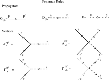
Figure 1: Summary of the Feynman rules. Solid line represents the propagator $G_{(0)}$ (Eq.(7)) for the correlated fermion $f_{p}$. Dashed line represents the $6\times 6$ boson propagator $D_{(0)}$ (Eq.(8)) for the $6$-component field $\delta X^{a}$. Note that the component $(1,1)$ of this propagator is directly associated with the $X^{00}$ charge operator. Doted line is the propagator $B$ for the boson ghost field ${\cal Z}_{p}$. $\Lambda^{pp^{\prime}}_{a}$ (Eq.(9)) and $\Lambda^{pp^{\prime}}_{ab}$ represent the interaction between two fermions $f_{p}$ and one and two bosons $\delta X^{a}$ respectively. $\Gamma^{pp^{\prime}}_{a}$ and $\Gamma^{pp^{\prime}}_{ab}$ represent the interaction between two ghost fields ${\cal Z}_{p}$ and one and two bosons $\delta X^{a}$ respectively.

The mean field values $r_{0}$ and $\Delta$ must be determined minimizing the leading order theory. From the completeness condition $r_{0}$ is equal to $\delta/2$ where $\delta$ is the hole doping away from half-filling. On the other hand, minimizing respect to $\Delta$ we obtain $\Delta=\frac{J}{2}\frac{1}{N_{s}}\sum_{k}cos(k_{x})n_{F}(E_{k}-\mu)$ where $n_{F}$ is the Fermi function and $N_{s}$ is the number of sites in the Brillouin zone (BZ).

For a given doping $\delta$, the chemical potential $\mu$ and $\Delta$ must be determined self-consistently from $(1-\delta)=\frac{2}{N_{s}}\sum_{k}n_{F}(E_{k}-\mu)$.

We associate with the six component $\delta X^{a}=(\delta R\;,\;\delta{\lambda},\;r^{x},\;r^{y},\;A^{x},\;A^{y})$ boson field, the inverse of the propagator, connecting two generic components a and b,

$$D^{-1}_{(0)ab}(q,\omega_{n})=N\left(\begin{array}[]{cccccc}(4V-2J)r_{0}^{2}(cos(q_{x})+cos(q_{y}))&r_{0}&0&0&0&0\\ r_{0}&0&0&0&0&0\\ 0&0&\frac{4}{J}\Delta^{2}&0&0&0\\ 0&0&0&\frac{4}{J}\Delta^{2}&0&0\\ 0&0&0&0&\frac{4}{J}\Delta^{2}&0\\ 0&0&0&0&0&\frac{4}{J}\Delta^{2}\end{array}\right)$$ (14)

The bare boson propagator $D_{(0)ab}$ (the inverse of Eq.(8)) is $O(1/N)$. As we will see $D_{0}$ is renormalized to $D$ by an infinite series of diagrams of $O(1/N)$.

We associate with the N-component ghost field ${\bf{\cal Z}}_{p}$, the propagator, connecting two generic components $p$ and $p^{\prime}$, $B_{pp^{\prime}}=-\delta_{pp^{\prime}}$ which is $O(1)$.

The expressions for three-leg and four-leg vertices are:

a)

$$\Lambda^{pp^{\prime}}_{a} = (-1)\;\left(\frac{i}{2}(\nu_{n}+{\nu^{\prime}}_{n})+\mu+2\Delta\sum_{\eta}cos(k_{\eta}-\frac{q_{\eta}}{2})\;cos\frac{q_{\eta}}{2};\;1;-2\;\Delta\;cos(k_{x}-\frac{q_{x}}{2})\;;\right.$$ (15)

$$- \left.2\;\Delta\;cos(k_{y}-\frac{q_{y}}{2});\right.\left.2\;\Delta\;sin(k_{x}-\frac{q_{x}}{2})\;;2\Delta\;sin(k_{y}-\frac{q_{y}}{2})\right)\;\delta^{pp^{\prime}}$$

represents the interaction between two fermions and one boson.

b) $\Lambda^{pp^{\prime}}_{ab}$, which represents the interaction between two fermions and two bosons, is a $6\times 6$ matrix where the only elements different from zero are:

$$\Lambda^{pp^{\prime}}_{\delta R\delta R} = \left(\frac{i}{2}(\nu_{n}+{\nu^{\prime}}_{n})+\mu+\Delta\;\sum_{\eta}cos(k_{\eta}-\frac{q_{\eta}+q^{\prime}_{\eta}}{2})\;[cos\frac{q_{\eta}}{2}\;cos\frac{q^{\prime}_{\eta}}{2}\;+\;cos\frac{q_{\eta}+q^{\prime}_{\eta}}{2}]\right)\delta^{pp^{\prime}}$$ (16)

$$\Lambda^{pp^{\prime}}_{\delta R\delta\lambda}=\frac{1}{2}\;\delta^{pp^{\prime}}$$ (17)

$$\Lambda^{pp^{\prime}}_{\delta R\;r^{\eta}}=-\Delta\;cos(k_{\eta}-\frac{q_{\eta}+q^{\prime}_{\eta}}{2})\;cos\frac{q^{\prime}_{\eta}}{2}\;\delta^{pp^{\prime}}$$ (18)

$$\Lambda^{pp^{\prime}}_{\delta R\;A^{\eta}}=\Delta\;sin(k_{\eta}-\frac{q_{\eta}+q^{\prime}_{\eta}}{2})\;cos\frac{q^{\prime}_{\eta}}{2}\;\delta^{pp^{\prime}}$$ (19)

c) $\Gamma^{pp^{\prime}}_{a}=(-1)(\delta_{pp^{\prime}}\;,\;0,\;0,\;0,\;0,\;0)$ represents the interaction between two ghosts and one boson.

d) ${\Gamma}^{pp^{\prime}}_{ab}$ is a $6\times 6$ matrix, where ${\Gamma}^{pp^{\prime}}_{{\delta}R{\delta}R}=\delta_{pp^{\prime}}$ and, the others components are zero. It represents the interaction between two bosons and two ghosts.

Each vertex conserves the momentum and energy and they are $O(1)$. In addition, in each diagram there is a minus sign for each fermion loop and a topological factor.

Fig.1 summarizes the Feynman rules.

After identifying the propagators and vertices and the respective order of them, in the next sections, we will calculate different physical quantities.

Before finishing this section, one remark is necessary. From the $N$-extended completeness condition we can see that the charge operator $X^{00}$ is $O(N)$, while the operators $X^{pp}$ are $O(1)$. This fact will have the physical consequence that the $1/N$ approach weakens the effective spin interactions compared to the one related to the charge degrees of freedom. This is discussed in the next section.

III Charge Correlations

In this section density-density correlations functions are calculated. It will be showed that the developed formalism can be used in explicit calculation of different correlation functions and we will also compare our results with others in the literature.

The density-density correlation function is defined as Lew ; Foussats

$$\tilde{D}_{ij}=\frac{1}{N}\sum_{pp^{\prime}}<T_{\tau}X^{pp}_{i}X^{p^{\prime}p^{\prime}}_{j}>$$ (20)

Using $\sum_{p}X^{pp}_{i}=N/2-X^{00}_{i}$ we find for $\tilde{D}$ in the Fourier space

$$\tilde{D}({\bf q},\omega_{n})=-N{(\frac{\delta}{2})}^{2}D_{\delta R\delta R}({\bf q},\omega_{n})$$ (21)

The charge correlation, in $O(1)$, needs the calculation of all $O(1/N)$ contributions to $D_{\delta R\delta R}({\bf q},\omega_{n})$. From the Dyson equation, $(D_{ab})^{-1}=(D_{(0)ab})^{-1}-\Pi_{ab}$, the dressed components $D_{ab}$ of the boson propagator can be found after the evaluation of the $6\times 6$ boson self-energy matrix $\Pi_{ab}$. Using the Feynman rules we may evaluate $\Pi_{ab}$ through the diagramas of Fig.2. Note that $D_{\delta R\delta R}$ is the element $(1,1)$ of the $6\times 6$ dressed propagator.

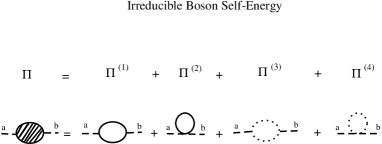
Figure 2: The four different contributions $\Pi^{(i)}_{ab}$ ($i=1,2,3,4$) to the irreducible boson self-energy $\Pi_{ab}$.

We note here an important difference with respect to the SBA. In SBA, only in leading order, the charge-charge correlation can be associated with the holon propagator. Beyond leading order, the convolution of holon propagators (which means the reconstruction of the $X$-operator $X^{00}$) is necessary. Meanwhile, in our case, it is not used any decoupling scheme and then, the different correlation functions are directly associated with our field variables.

The density-density spectral function, which in principle can be measure with electron energy loss scattering EELS , is defined as $D({\bf q},\omega)=-Im[\tilde{D}({\bf q},\omega)]$. The imaginary part is taken as usual after performing the analytical continuation $i\omega_{n}=\omega+i\eta$.

In Fig.3 we show the density-density correlation function for the physical value $J=0.3$ and for doping $\delta=0.20$. We plotted the densities for different ${\bf q}$ vectors in the BZ as a function of $\omega$. The ${\bf q}$ vectors and the physical parameters are the same to those used in the calculation of the densities in Ref.[Zeyher2, ]. We used $\eta=0.1$ in the analytical continuation.

Comparing Fig.3 with Fig.3 of Ref.[Zeyher2, ], we find a remarkable agreement between both methods in spite of the fact that the two approaches are very different.

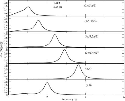
Figure 3: Density-density correlation functions for $J=0.3$, $V=0.0$ and $\delta=0.20$ for different ${\bf q}$’s in the BZ. The density-density correlation functions contain collective peaks due to infinite diagram summation seen in Fig.2. The collective peaks are well pronounced when they are above the particle-hole continuum (see for example ${\bf q}=(\pi,0)$). They are less pronounced when they are superimposed to the particle-hole continuum (see for example ${\bf q}=(2\pi/5,\pi/5)$). $\omega$ is in units of $2t$ and $t$ is considered to be $1$.

The density-density correlation function is nearly independent of $J$. For example, comparing Fig.3 (for J=0.3) with Fig.2 in Ref.[Foussats, ](for $J=0$) for momentum ${\bf q}=(\pi,\pi)$, we find a well pronounced collective peak (or zero sound) at $\omega\sim 3.5$. (Note that in Ref.[Foussats, ] $\omega$ is in units of $t$ meanwhile in Fig. 3 it is in units of $2t$ in order to absorb the factor $1/N$ due to the re-scaling of the hopping term.)

The fact that the density correlations are nearly independent of $J$ means that $\tilde{D}({\bf q},i\omega_{n})$ is dominated by charge fluctuations. As we mentioned above, the present formalism privileges charge over spin fluctuations. Another consequence of this result is the absence, in $O(1)$, of collective excitations (like magnons) in the spin susceptibility. The spin-spin correlation function is the electronic bubble with renormalized band due to correlations Foussats ; Lew . Meanwhile there are collective effects in the charge sector in $O(1)$, that appear in $O(1/N)$ in the spin sector.

The collective peaks are more pronounced when they are present well above the particle-hole continuum as for ${\bf q}=(\pi,\pi)$. For momentum ${\bf q}=(2\pi/5,\pi/5)$ the collective peak is superimposed to the particle-hole continuum and it appears broader. The broadening of the collective peak ${\bf q}=(\pi,\pi)$ is not intrinsic and it is only due to the finite value of $\eta$ we used in the analytical continuation.

At this point we can compare our results with those obtained using exact diagonalization Tohyama . Despite the charge correlation function in Ref.[Tohyama, ] was for doping $\delta=0.25$ and $J=0.4$ and our calculation is for $\delta=0.20$ and $J=0.3$, there are some similarities and differences to remark. For example, Fig. 2 in Ref.[Tohyama, ] shows also a peak at ${\bf q}=(\pi,\pi)$. However, a) this peak appears at larger energies than our collective peak, b) the peak at $(\pi,\pi)$ obtained in Ref.[Tohyama, ] contains more structure than the ours and c) we must note also a difference at ${\bf q}=(\pi,0)$. In our calculation we found a collective-like peak at $\omega\sim 2$ and a broad and small continuum at low energy. Lanczos diagonalization presents also this picture but, in addition there is a peak at lower energy. As it was already pointed out by Khaliullin and Horsch in Ref.[Kha1, ] (see also Ref.[Kha2, ]), the inclusion of fluctuations beyond the mean field level is probably responsible for the differences listed in a), b) and, c). We think that the inclusion of fluctuations is more important at lower than at larger doping. In Ref.[Merino, ], for doping $\delta=0.5$, we found a better agreement between the peak position for ${\bf q}=(\pi,\pi)$ obtained by our approach and that obtained by Lanczos.

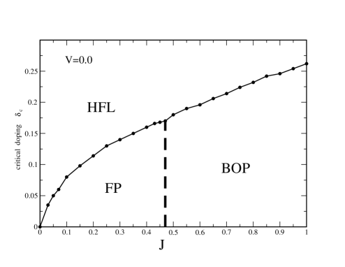
Figure 4: Phase diagram in the $\delta_{c}-J$ plane for $V=0.0$. The solid line defines the stability border for the homogeneous Fermi liquid (HFL). For a given $J$ the HFL is stable for $\delta>\delta_{c}$. The thick dashed line around $J\sim 0.5$ separates the flux phase (FP) from the bond order phase (BOP).

IV Instabilities

IV.1 Flux and Bond-Order phases

The theory developed in previous sections defines a homogeneous Fermi liquid (HFL) phase. In $O(1)$ the mean field solution ($r_{0}$, $\Delta$) was independent of sites. Therefore, at $N$-infinite, we have free fermions with renormalized band $E_{k}$ due to correlations.

In this section we will study the stability conditions for the HFL.

In leading order, there are collective effects in the charge sector whereas there are not in the spin sector. Therefore, in principle, we expect instabilities in the charge channel.

The HFL system is unstable when the static charge susceptibility $Re(\tilde{D}({\bf q},i\omega_{n}=0)$ diverges. The ${\bf q}$ vector, where the instability occurs ($\bf{q_{c}}$), being the modulation of the new phase.

Fig.4 shows the phase diagram of the model for $V=0$. For a given $J$, below a critical doping $\delta_{c}$ where the static charge susceptibility diverges at a given vector ${\bf q}$ in the BZ, the HFL is not the stable phase.

In the limit $J\rightarrow 0$ $\delta_{c}\rightarrow 0$ the HFL is stable for the whole doping range except at half filling where the system is an insulator because the band effective-mass tends to infinite.

The instability is placed, for all $J$, on the border of the BZ. That is, ${\bf q_{c}}=(1,x)\pi$ or ${\bf q_{c}}=(x,1)\pi$ where the parameter $x$ measures the degree of the incommensuration of the instability.

In Fig.5 we plot the incommensuration $x$ as a function of $\delta_{c}$. For $\delta_{c}\rightarrow 0$, $x\rightarrow 1$. Therefore, in the limit of $J\rightarrow 0$, we found a phase with commensurate order ${\bf q_{c}}=(\pi,\pi)$.

It is easy to overlook the instability just by looking at the static charge susceptibility. In Fig.6 we plot the static charge susceptibility, along ${\bf q}=(\pi,q)$, for $\delta=0.15$ and $\delta=0.14$ and, for the physical value $J=0.3$. From Fig.4 we know that the HFL is not stable for doping $\delta=0.14$ whereas for $\delta=0.15$ it is stable. Both curves in Fig.6 look similar and, for $\delta=0.14$ there is no indication of the instability for ${\bf q}\sim{\bf q_{c}}$ because it occurs in a very narrow region of momentum near ${\bf q_{c}}$. In practice, this means that the set of ${\bf q}$-points in Fig.6 is not dense enough to localize the divergence of $Re(\tilde{D}({\bf q},i\omega_{n}=0))$. As we will see below, this is related with the fact that the instability is weakly coupled with the charge sector.

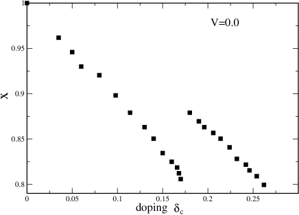
Figure 5: Inconmensuration $x$ vs $\delta_{c}$ for $V=0.0$. $x$ is defined as ${\bf q_{c}}=(1,x)\pi$. ${\bf q_{c}}$ is the ${\bf q}$-vector where the instability takes place. The instability is incommensurate for all $J$ except for $J\rightarrow 0$ where $x\rightarrow 0$ (${\bf q_{c}}\rightarrow(\pi,\pi)$). At the separating border of the FP from the BOP there is a jump in the value of ${\bf q_{c}}$.

To calculate $\tilde{D}({\bf q},\omega_{n})$ we have to evaluate the inverse of $(D_{ab})^{-1}$. Therefore, for a better determination of the instability, we may look for the zeros of the determinant of $D_{ab}^{-1}$. In the inset of Fig.6 we plot the $det(D^{-1}_{ab})$ as a function of ${\bf q}=(\pi,q)$. For $\delta=0.14$ (close to the onset of the instability) the determinant changes sign in a narrow region around ${\bf q_{c}}\sim(\pi,2.7)$ making the HFL unstable. Meanwhile, for $\delta=0.15$ the determinant is positive for all q and the system is stable. A similar plot for $\delta<0.14$ shows, of course, a larger negative region for $det(D_{ab}^{-1})$.

In order to characterize the nature of the new phase, we have studied the eigenvector corresponding to the zero eigenvalue of $(D_{ab})^{-1}$.

For doping $\delta<\delta_{c}\sim 0.5$ the eigenvector corresponding to the zero mode is $\sim(0,0,0,0,-1,1)$. Then, in the new phase, the 5th and 6th components of $\delta X^{a}$ ($A^{x}$ and $A^{y}$) are frozen. $A^{x}$ and $A^{y}$ are associated with the phase of the field $\Delta^{\eta}$ and they take opposite values. Therefore, as the instability occurs near the momentum $(\pi,\pi)$, this new phase is the well known flux phase (FP) Marston ; Capellutti which opens a gap, with $d$-wave symmetry in the normal state.

Recently, Chakravarty, Laughlin, Morr and Nayak considered that the FP or DDW as a candidate to explain the physics of the pseudogap in underdoped cupratesChakra .

The first component of the eigenvector corresponding to zero eigenvalue is not zero exactly. It has a small value which means that the FP is weakly coupled to the charge sector. It means that the DDW is not completely hidden when it is incommensurate. Although Bragg peaks are predicted, they will show low intensity which would make their observation very difficult. This is the reason by which, any charge-probe is not very sensitive to show the FP instability. When ${\bf q_{c}}$ is exactly $(\pi,\pi)$ the eigenvector does not have any mixing with the charge sector and, the flux phase is fully hidden.

For doping $\delta>\delta_{c}\sim 0.5$ the unstable eigenvector is of the form $\sim(0,0,0,1,0,0)$. This state is known as bond-order phase (BOP) Capellutti ; Lubenski .

In the range of the studied parameters we did not find indications for phase separation.

In Fig.5, for $J\sim 0.5$, near the crossover from the FP to BOP, there is a jump in the incommensuration $x$.

The agreement with other methods Capellutti ; Lubenski is again remarkable in spite of the fact that the present approach is, a priori, very different from those ones. Taking into account that we constantly find similar or even the same results by means of different methods turn the results reliable. For example, for the physical value $J=0.3$, the HFL is unstable against a FP. This result is very robust and, many different methods agree that the stable phase, for small doping, is a FP for the physical region of the parameters Marston ; Grilli ; Lubenski ; Capellutti ; Numerics .

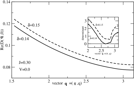
Figure 6: Static charge susceptibility $Re(\tilde{D}({\bf q},i\omega_{n}=0))$ vs ${\bf q}=(\pi,q)$ for $J=0.3$, $V=0.0$ and, for $\delta=0.15$ and $\delta=0.14$. For $\delta=0.14$ (solid line) the curve looks similar to the case for $\delta=0.15$ (dashed line). For $\delta=0.14$ the HFL is not stable and there is no strong sign of the instability in the static charge susceptibility. In the inset we plot the $det(D_{ab}^{-1})$ (see text for discussions) vs ${\bf q}=(\pi,q)$. For $\delta=0.14$, the $det(D_{ab}^{-1})$ clearly changes sign in a small region around ${\bf q_{c}}\sim(\pi,2.7)$.

IV.2 Charge Density Wave phase

The inclusion of a nearest-neighbors Coulomb repulsion $V$ favors a charge density wave (CDW) state. In order to investigate this instability, we have included a finite value of $V$ in the calculation.

The study of a nearest-neighbors Coulomb repulsion in correlated models is important. In cuprates, there are indications Fein showing the existence of $V$ with a value close to $J$. If $J$ favors superconductivity and, the value of $V$ is large, it is reasonable to think that superconductivity will be diminished due the presence of $V$. There are some analytical and numerical works studying the competition between $V$ and $J$ on superconductivity. Meanwhile some papers indicate that superconductivity in the $t-J$ model vanishes for $V\sim J$ Zeyher1 , others indicate that superconductivity survives up to values of $V>>J$ Riera .

On the other hand, the presence of $V$ seems to be important for understanding the physics of organic materials jaimes . Some peculiarities in the optical conductivity (and also superconductivity) occur near the charge order and this picture can be interpreted by the competition between $V$ and the kinetic energy in correlated models org .

Looking at the Eq.(8) we see that $V$ is only present in the element $D^{-1}_{(0)}(1,1)$. The Coulomb term enters in our approach multiplied by $(\delta/2)^{2}$ which means that the effect of $V$, at low doping, is strongly screened by the correlations.

We note that in the SBA $V$ can enter in different manners depending on the way chosen for the decoupling.

In Fig.7 we show the phase diagram in the $V_{c}-\delta$ plane for J=0 and $J=0.3$. The curves show, as a function of $\delta$, the critical Coulomb repulsion $V_{c}$ where the CDW instability takes place. For $V<V_{c}$ the HFL is stable. This result is in agreement with numerical Merino and analytical methods Hoang . In Ref.[Hoang, ] the authors use coherent potential approximation and their results are close to the ours.

A similar result was also recently found, at $J=0$, in the triangular lattice in the context of the new low dimensional superconductor $Na_{x}CoO_{2}$ Lee .

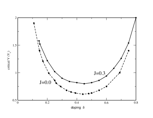
Figure 7: Charge density wave (CDW) stability line $V_{c}$ vs $\delta$ for $J=0.0$ (dashed line) and $J=0.3$ (solid line). For a given $\delta$, the system is in a CDW state for $V>V_{c}$. The value of $V_{c}$ increases with increasing $J$. For $J=0.3$ the first presented doping is $\delta=0.15$. (For $J=0.3$ the HFL is not stable for $\delta<0.14$ at $V=0.0$).

For $J=0.3$ and doping $\delta=0.20$, the HFL is stable at $V=0$. When $V=V_{c}\sim 1.25$ the system enters in a CDW state. This $V_{c}$ is $\sim$ $40\%$ larger than for $J=0$ and the same doping. There are two sources for this tendency.

a) When $J$ is finite, there is a contribution $\Delta$ to the effective hopping in $E_{k}$. Then, the system win kinetic energy when $J$ is finite and, a larger $V$ is necessary in order to localize the charges.

b) As we see in the element $(1,1)$ of $D^{-1}_{(0)}$, the effect of $V$ is diminished when $J$ is finite. The term $2J$ in the element $(1,1)$ comes from the charge-like term $J_{ij}X_{i}^{\sigma\sigma}X_{j}^{\bar{\sigma}\bar{\sigma}}$ of the pure $t-J$ model, which is of the same form of the Coulomb term (see Eq.3).

In order to identify the main source for the increasing of $V_{c}$ we looked for the CDW instability without the charge-like term in (3). Under this condition, for $J=0.3$ and $\delta=0.20$, $V_{c}$ is $V_{c}\sim 1.0$. This value is nearly the same than $V_{c}$ for $J=0$. Therefore, b) is the main source for the increasing of $V_{c}$ with increasing $J$.

In contrast to the FP and BOP, the CDW instability can be detected clearly by looking at the static charge susceptibility $Re(\chi({\bf q},i\omega_{n}=0))$.

In Fig.8 we show, for $J=0.3$ and $\delta=0.25$, $Re(\chi({\bf q},i\omega_{n}=0))$ vs ${\bf q}=(q,q)$ for $V=1.$ (a little smaller than the critical value $1.1$) and $V=0.5$. In the figure, we see that approaching $V_{c}$, the static susceptibility tends to diverge near ${\bf q}=(\pi,\pi)$. For $V=0.5$ ($V<<V_{c}$), the static charge susceptibility is flat.

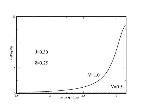
Figure 8: Static charge susceptibility for $J=0.3$ and $\delta=0.25$ vs ${\bf q}=(q,q)$ for two different values of $V$, $V=1.$ and $V=0.5$. $V=1.$ is near (from below) the value of $V_{c}=1.1$. In contrast to Fig.6, the CDW instability has a clear signal in the static charge susceptibility. For $V=1.$ there is a clear indication of a divergence at $(\pi,\pi)$. For $V=0.5$ ($V<<V_{c}$), the static charge susceptibility is flat.

In this case the eigenvector corresponding to the zero eigenvalue is $\sim(1,0,0,0,0,0)$. Then, the instability is mainly in the pure charge sector.

From Fig.8, in agreement with other methods Merino , the instability ${\bf q}$-vector is always at ${\bf q}=(\pi,\pi)$. Therefore, in the CDW phase, the charges order themselves forming a checkerboard pattern. For doping different to the commensurate one $\delta=0.5$ we must interpret the CDW instability as the system is charge-ordered but remains metallic. These results were obtained by different methods and the nature of the instability for doping different to the commensurate one is still open. For the commensurate doping $\delta=0.5$ in Ref.[Merino, ] we showed that the system is charge-ordered at $V_{c}\sim 0.6$ however, we also find an insulator because the quasiparticle weight goes to zero exactly at this $V_{c}$ value.

In order to compare the above results to the predictions of the BKF method, we calculated the critical $V_{c}$ using the formulation of Refs.[Zeyher, ] [Zeyher1, ] for $J=0.3$. For $\delta=0.20$ and $\delta=0.60$ we found $V_{c}\sim 1.25$ and $V_{c}\sim 0.9$ respectively. The agreement with our calculation is again very good in spite of the fact that the Coulomb term enters BKF in a different way.

V Conclusions

From the path integral representation for the Hubbard $X$-operators we have developed a new perturbative theory for the $t-J-V$ model. Our formulation is free of slave-particles and the $X$-operators are treated as fundamental objects.

We have extended the large-$N$ formalism, recently developed in Ref. [Foussats, ], to the case of finite $J$.

To work directly with the $X$-operators has several advantages upon the slave-particles methods. For example, in the slave-boson theory, the decoupling procedure introduces a gauge degree of freedom and then, an additional problem as the gauge fixing arises. This problem does not occur in our formulation. On the other hand, in the slave approaches, in contrast to our method, beyond a mean field level, a convolution between slave-particles propagators is necessary to reconstruct the original physical propagator.

Fig.1 summarizes the Feynman rules of the present approach where the propagators and vertices are written in terms of the Hubbard operators $X^{\sigma 0}$, $X^{00}$, etc.

It is important to note that we can not read the interaction vertices from the $t$ and $J$ terms of the Hamiltonian. They arise from the nonpolynomial effective theory defined by $L_{eff}$ in Eq.(6). All the interactions caused by the Hubbard algebra (commutation rules and constraints) were transfered to $L_{eff}$.

The formalism developed in the present paper privileges charge over spin fluctuations. While there are collective effects in the charge sector in $O(1)$, those appear in $O(1/N)$ in the spin sector.

We have studied charge correlations functions and we have investigated the role of collective effects. This study shows the presence of collective peaks (or zero sound) which are more evident when they are separated from the particle-hole continuum. On the other hand, the collective peaks become broader when they are superimposed to the particle-hole continuum. One important characteristic of the charge correlation function is the fact that this is not strongly dependent on the value of the exchange interaction $J$.

At large $N$, the theory can be described as a homogeneous Fermi liquid with renormalized band due to correlations. We have studied the stability of this Fermi liquid phase. For a given value of $J$, the Fermi liquid phase is stable for doping $\delta>\delta_{c}$. The critical doping $\delta_{c}$ decreases with decreasing $J$. For doping below $\delta_{c}$ the system enters in a flux or bond order phase depending if $J<0.5$ or $J>0.5$ respectively. These instabilities are weakly coupled to the charge sector which means that any charge-probe is not an efficient test to detect them. One important characteristic of these new phases is that they are incommensurate with a modulation vector ${\bf q}=(1,x)\pi$ where the incommensuration $x$ tends to $1$ when $J$ goes to zero.

It is important to remark that in agreement with other theories, for low doping, the Fermi liquid is unstable against a flux or $d$-density wave phase for the physical region of the parameters.

We also have investigated the role of a nearest-neighbors Coulomb repulsion $V$ on the stability conditions of the Fermi liquid. When $V$ is larger than a critical value $V_{c}$, the system enters, at a given doping, in charge density wave state. The value of $V_{c}$ increases with increasing $J$. We have identified in the charge-like term of the pure $t-J$ model the main reason for this increase.

We have continuously compared our results with similar ones in the literature. The agreement of our results with those obtained by other methods give confidence to the results and the approach of the present paper.

At leading order, our formalism is in agreement with the slave-boson approach. However, at the next to leading order (which is necessary to calculate dynamical properties) the differences between the two formulations are not yet completely established. We think that the complications that appear in the slave-boson method beyond mean field level as gauge fixing, Bose condensation, regularizing factors Arrigoni are not good for the advance of the field. In our case we do not have these problems and we think that our approach can be useful to go beyond the mean field level. With the formulation for finite $J$ in hand, we expect to continue in this direction as we did for $J=0$ in Ref.[Merino, ].

Acknowledgments

The authors thank to C. Genz, L. Manuel, J. Merino and R. Zeyher for valuable discussions.

References

- (1) P.W. Anderson, The Theory of Superconductivity in High- Cuprates (Princeton University Press, Princeton,1997).
- (2) R.H.McKenzie, Science 278,820(1997).
- (3) A. Izyumov, Physics-Uspekhi 40, 445 (1997).
- (4) E. Dagotto, Rev.Mod.Phys. 66,763(1994).
- (5) J. Hubbard, Proc. R. Soc. London Ser. A 276, 238 (1963).
- (6) E. Arrigoni et al, Phys. Rep.241, 291(1994).
- (7) Z. Wang, Int. Journal of Modern Physiscs B 6, 155(1992).
- (8) R. Zeyher and M. L. Kulić, Phys.Rev. B 53, 2850(1996).
- (9) R. Zeyher and A. Greco, Eur. Phys. J.B 6, 473 (1998).
- (10) A. Foussats, A. Greco, C. Repetto, O. P. Zandron and O. S. Zandron, Journal of Physics A 33, 5849(2000).
- (11) A. Foussats and A. Greco; Phys.Rev.B65, 195107(2002).
- (12) J. Merino, A. Greco, R. H. McKenzie, and M. Calandra, Phys. Rev. B 68, 245121(2003).
- (13) L. Gehlhoff and R. Zeyher, Phys. Rev. B52, 4635(1995).
- (14) E. Zojer, M. Knupfer, Z. Shuai, J. Fink, J.L. Bredas, H. H. Horhold, J. Grimme, U. Scherf, T. Benincori, and G. Leising, Phys.Rev.B 61,16561(2000).
- (15) R. Zeyher and M. L. Kulić, Phys.Rev. B 54, 8985(1996).
- (16) T. Tohyama, P. Horsch and S. Maekawa, Phys. Rev. Lett. 74, 980(1995).
- (17) G. Khaliullin and P. Horsch; Phys.Rev. B 54, R9600(1996).
- (18) P. Horsch and G. Khaliullin; cond-mat/0312561 (2003).
- (19) I. Affleck and J.B. Marston, Phys.Rev.B37,3774(1988).
- (20) E. Cappelluti and R. Zeyher, Phys.Rev.B59, 6475(1999).
- (21) S. Chakravarty, R. B. Laughlin, D.K.Morr, and Ch. Nayak, Phys. Rev. B 63,94503 (2001).
- (22) M. Grilli and G. Kotliar, Phys.Rev. Lett. 64, 1170 (1990).
- (23) D.C. Morse and T.C. Lubensky, Phys.Rev. B 42,7994(1990).
- (24) P.W.Leung, Phys. Rev. B62,6112(2000).
- (25) L.F. Feiner,J.H.Jefferson and R. Raimondi, Phys.Rev. B 53 8751 (1996).
- (26) J. Riera and E. Dagotto, Phys.Rev.B 57,8609 (1998); M. Calandra and S. Sorella, Phys. Rev. B61,11894(2000); C. Gazza, G.B. Martins, J. Riera and E. Dagotto, Phys.Rev.B 59, 709(1999).
- (27) R.H.McKenzie,J.Merino,J.B.Marston and O.P.Sushkov, Phys.Rev.B64,085109(2001); J.Merino and R.H.McKenzie, Phys.Rev. Lett. 87,237002(2001).
- (28) M.Dressel, N.Drichko, J.Schlueter, and J. Merino, Phys.Rev.Lett.90,167002(2003).
- (29) A.T. Hoang and P.Thalmeier, J. Phys.: Condens. Matter 14 6639(2002).
- (30) O. Motrunich and P. Lee, Phys. Rev.B70,024514(2004).