A unifying model for several two-dimensional phase transitions

Abstract

A relatively simple and physically transparent model based on quantum percolation and dephasing is employed to construct a global phase diagram which encodes and unifies the critical physics of the quantum Hall, ”two-dimensional metal-insulator”, classical percolation and, to some extent, superconductor-insulator transitions. Using real space renormalization group techniques, crossover functions between critical points are calculated. The critical behavior around each fixed point is analyzed and some experimentally relevant puzzles are addressed.

Two-dimensional phase transitions have been a focus of interest for many years, as they may be the paradigms of second order quantum phase transitions (QPTs). However, in spite of the abundance of experimental and theoretical information, there are still unresolved issues concerning their behavior at and near criticality, most simply exposed by the value of the critical exponent $\nu$ (describing the divergence of the correlation length at the transition). Below we discuss three examples which underscore these problems. First, in the integer quantum Hall (QH) effect, which is usually described within the single particle framework, various numerical studies yielded a critical exponent $\nu\approx 2.35$ QHnumerics , in agreement with heuristic arguments milnikov . Some experiments indeed reported values around $2.4$ exp2.4 , while other experiments reported exponents around $1.3$ exp1.3 , close to the classical percolation exponent $\nu_{p}=4/3$. Even more perplexing, some experiments claim that the width of the transition does not shrink to zero at zero temperature noncritical , in contradiction with the concept of a QPT. Additionally, the observation of a QH insulator QHinsulator is inconsistent with the QPT scenario assa . Consider secondly the superconductor (SC) - insulator transition (SIT), for which theoretical studies suggest several scenarios. Similar to the QH situation, some experiments yield a value $\nu\approx 1.3$ SC1.3 , not far from the value $\nu\simeq 1$, predicted by numerical simulations within the random boson model, but closer to the classical percolation value. Other experiments, however, yield $\nu\simeq 2.8$ SC2.8 , while some experiments claim an intermediate metallic phase metallic . As a third example, consider the recently claimed metal-insulator transition (MIT) mit . The critical exponent is again close to $1.3$ meir ; dassarma but the occurrence of such phase transition is in clear contrast with the scaling theory of localization.

The basic question which naturally arises is then whether it is possible to unify these two dimensional phase transitions within a single theory and thereby resolve some of the problems raised above. A hint toward an affirmative answer is gained by experimental indications that percolation plays a key role in both the QH transition QHperc and in the SIT SIperc . Moreover, its relevance to the MIT has been argued theoretically and observed experimentally meir ; dassarma ; xi . The QH and the SIT have been treated within a percolation-like model in Ref. kapitulnik , consisting of SC or QH droplets connected via quantum tunneling, similar in spirit to the model presented in model .

In the present work we address these issues using a physically transparent picture. A similar approach proved to be quite successful for developing a model encoding the QH transition which can also describe some aspects of the SIT model . Introducing a new aspect, decoherence, into the model, we are able to include the QH transition (or the SIT), classical percolation and the MIT all within the same phase diagram. Employing real-space renormalization group (RSRG) techniques, we first calculate the critical exponents. Most important, we employ this phase diagram for understanding the possible critical features, and expose the physical conditions necessary to observe them. The crossover between different critical points, which may be explored experimentally is investigated and concrete experimental predictions are made.

For the sake of self-consistence, the model used to describe the QH effect model , is briefly explained here. In high magnetic fields, electrons follow equi-potential lines, which, at low Fermi energy, are trapped in potential valleys. At zero temperature, transport through the system is due to quantum tunneling between such trapped trajectories. Within the model, this picture is mapped on a lattice such that each closed trajectory in a valley corresponds to a site, and quantum tunneling between (nearest neighbor) sites corresponds to a (quantum) link. As the Fermi energy rises and crosses the saddle point separating two isolated contours, these two trajectories merge into one. The transmission between these two sites becomes perfect, and the link connecting them is considered SC. The QH transition point occurs when such a trajectory spans the entire system, which, in the model corresponds to percolation of the SC links. Consequently, the QH problem maps onto a lattice, with random tunneling amplitudes between its sites, and a finite fraction of perfect bonds, namely a mixture of quantum and SC links. The critical behavior of the QH is encoded by the scaling behavior near the percolation point of this lattice model. Calculation of the transmission through such a system, using two different approaches, yielded a diverging localization length, with an exponent $\nu\approx 2.4\pm 0.1$, close to the results of other numerical estimatesQHnumerics .

The new element introduced into the model is dephasing. A fraction $q$ of the links is attached to current conserving phase disrupting reservoirs buttiker . Physically, it is a consequence of finite temperature but can result from other mechanisms. An electron propagating along such a link enters the reservoir and loses its phase, before it, or another electron, emerges from the reservoir (there is no net current into the reservoir). Transport along this link is therefore incoherent. Transmission in the presence of such phase breaking resistors can be treated within the Landauer-Buttiker formalism. The model parameters are then $p$, the fraction of SC links (i.e quantum links whose transmission is unity), and $q$, the fraction of classical, or incoherent links. Evidently, the fraction of quantum tunneling links is $1-p-q$. The principal objective is then to construct a phase diagram in the ($p,q$) plane of parameters and to identify the various critical transitions in this plane.

Our main tool will be the RSRG scheme on a square lattice. In order to gain experience and confidence we first perform calculations on the line $q=0$ which reduces to our previous, fully coherent model as a special case. Rescaling the lattice by a factor of 2, each $2\times 2$ square is mapped onto a $1\times 1$ square (Fig 1a). Given the transmission amplitude of each link in the $2\times 2$ square, we evaluate the transmission through the whole unit, by attaching leads to its left and right sides (see below). This will allow us to follow the distribution of the transmission amplitudes from one iteration to another, and eventually evaluate the distribution for the full lattice. For the classical problem this calculation reduces to the calculation of transport through a Wheatstone bridge (Fig. 1b), where the symmetry of the square lattice has been used. For simplicity we use the Wheatstone bridge geometry for the quantum problem, and later verify that the addition of dangling bonds does not modify the critical behavior.

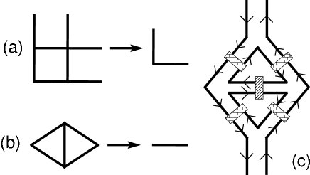
Figure 1: The real-space renormalization group process on a square lattice. (a) The mapping of a $2\times 2$ square onto a $1\times 1$ square, resulting in reducing the size of the lattice by a factor of $2$. (b) The equivalent mapping for which the calculation has been done. For the classical problem this equivalence is exact, while for the quantum problem it neglects the effects of dangling bonds. Later in the calculation dangling bonds have been included with no observable change in the critical behavior. (c) The scattering matrix approach (rotated 90 degrees compared to (b)). At each junction each edge state propagates freely according to its chirality. Scattering is along the links (marked as partially filled rectangles across the links). It is easy to see that if there is a percolating path of perfect scatterers (scatterers with unit transmission), then there is a perfect transmission along the whole structure.

The actual calculation is carried out using the scattering matrix approach. Each link carries a left going and a right going channel. In accordance with the physics at strong magnetic fields there is no scattering in the junctions (valleys) and the edge state continues uninterrupted according to its chirality (see Fig. 1c), while the scattering occurs on the link (saddle point) itself. Each scatterer is characterized by its scattering matrix $S_{i}$, namely a transmission probability $T_{i}$ and phases. For each realization of transmission probabilities on the larger lattice, we can evaluate exactly the transmission through the whole lattice $\hat{T}(\{T_{i}\},\phi)$ , and thus follow its distribution from one iteration to another, allowing us to determine the fixed points and the RSRG flow. If one starts with a distribution of scattering matrices whose phases are uniformly distributed, they remain so, and thus we will be only interested in the scaling of the distribution of the transmission probabilities,

$$G^{\{n\}}(T)=\int\ldots\int\ \delta\left(T-\hat{T}(T_{1},\ldots,T_{5},\boldsymbol{\phi})\right) \times$$

$$\times\ G^{\{n-1\}}(T_{1})\cdots G^{\{n-1\}}(T_{5})\ dT_{1}\cdots dT_{5}\ d\boldsymbol{\phi},$$ (1)

where $\boldsymbol{\phi}$ stands for all the independent phases.

The initial distribution can be written as

$$G^{\{0\}}(T)=p\ \delta(T-1)+(1-p)\hat{G}^{\{0\}}(T),$$ (2)

where $p$ is determined by the fraction of saddle-point energies that are below the Fermi energy, $p(\epsilon_{F})=\int_{-\infty}^{\epsilon_{F}}F(\epsilon)d\epsilon$, with $F(\epsilon)$ the distribution of the saddle point energies. $\hat{G}^{\{0\}}(T)$ is determined by the relation between the transmission and the saddle-point energy and by $F(\epsilon)$. The initial distribution $\hat{G}^{\{0\}}(T)$ does not affect the critical behavior, as the distribution always flows toward one of three possible fixed-point distributions.

Since the probability that the transmission is unity is determined by the classical percolation probability, one finds

$$G^{\{n\}}(T)=P_{n}(p)\delta(T-1)+\left(1-P_{n}(p)\right)\hat{G}^{\{n\}}(T,p),$$ (3)

where $P_{n}(p)$ is the classical percolation probability after $n$ iterations, and $\hat{G}^{\{n\}}$ can be exactly expressed in terms of $\hat{G}^{\{n-1\}}$. Clearly, if $p<p_{c}$, $P(p)$ flows toward zero, while for $p>p_{c}$ it flows to unity. At $p=p_{c}$ the distribution $\hat{G}$ flows toward a two-peak fixed distribution, similar to previously obtained results for the QH transition distribution . The critical behavior can be deduced by investigating the length dependence of the averaged transmission near the critical point and its collapse using $T(p,L)=T[L/\xi(p)]$, where $\xi(p)$ is an energy (or concentration) dependent localization length. We find that $\xi(p)$ diverges at $p_{c}=1/2$ with an exponent $\nu=2.4\pm 0.1$, consistent with previous numerical calculations for the QH transition QHnumerics .

Having demonstrated the power of the RSRG technique for $q=0$ (no dephasing) we now treat the model at an arbitrary point ($p,q$). Qualitatively, several phase transitions can be identified. For $q=0$ the QH transition is recovered as demonstrated above. For $p+q=1$ (no quantum links) the point $q=p_{c}={\small{1}\over{2}}$ describes the classical conductor-superconductor percolation transition. For the case of $p=0$, all the links are either quantum (with $T<1$) or classical. This is the model suggested in Refs. meir ; xi to describe the ”apparent” metal-insulator transition in two dimensions. The flow lines can be determined without the full quantum calculations by noticing that the rescaled cell will be SC if a cluster of SC links percolate, while it will be an incoherent metal if there is percolation of classical links, and no percolation of SC ones. These conditions define the RSRG equations for the quantities $p$ and $q$,

$$p^{\prime} = 2\,{\left(1-p\right)}^{3}\,p^{2}+8\,{\left(1-p\right)}^{2}\,p^{3}+5\,\left(1-p\right)\,p^{4}+p^{5}$$ (4)

$$q^{\prime} = q\left\{10p^{4}-20p^{3}\left(1-q\right)+2p\left(1-q\right)\left[2+5\left(1-q\right)q\right]\right.$$

$$+ \left.q\left(2+2q-5q^{2}+2q^{3}\right)+2p\left(2+3q-10q^{2}+5q^{3}\right)\right\}$$

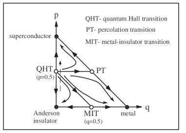
Figure 2: The phase diagram of the model in term of the parameters $q$, the concentration of a perfect-transmission links and $p$, the probability of incoherent links. The phase diagram displays three different phase transitions between the three different phases. The broken line represent a possible experimental trajectory leading to a finite metallic phase.

The full phase diagram thus contains three limiting phases, an Anderson insulator, a superconductor (or a QH phase) and an incoherent metal, and is depicted in Fig. 2. The fact that for $p>{\small{1}\over{2}}$ one gets a QH phase is straightforward, as once there is percolation of SC links there is an edge state propagating without backscattering through the system. The transition between an Anderson insulator and an incoherent metal is more intriguing. Once $p+q>{\small{1}\over{2}}$ an electron can propagate freely from one side of the system to the other, but necessarily goes through incoherent scattering, and thus this phase is an incoherent metal. For $p+q<{\small{1}\over{2}}$, however, there is no trajectory that allows the electron to traverse the system without quantum tunneling. These tunneling events, however, are intertwined with incoherent scattering, and thus the conductance of the system will be of the order of $\exp(-L_{\phi}/\xi)$, where $L_{\phi}\sim q^{-1/2}$ is the average distance between incoherent scattering events. As $q$ decreases, the conductance of the system goes to zero, ending up as an Anderson insulator. For finite $p$, however, the existence of incoherent scattering is not expected to affect the quantization of the Hall conductance efrat . Thus one may characterize the phase with finite $p$ and $q$, but with $p+q<{\small{1}\over{2}}$ as a ”Hall insulator”. In agreement with previous treatments of this phase, we also conclude that it only exists for finite dephasing ($q>0$), as for $q=0$ the system flows to an Anderson insulator. Further investigation of this phase will be reported elsewhere.

Beyond the characterization of the different phases, the model allows a direct calculation of the crossover between them. The line at $p={\small{1}\over{2}}$ allows, as a function of $q$, to study the crossover between the quantum SIT (or the QH transition) to the classical superconductor-conductor transition. Following the RSRG flow along this line, we find that the average transmission obeys

$$T(q,p={1\over 2})=T_{0}\left(1+\beta\left({L\over{L_{\phi}(q)}}\right)^{0.91}\right),$$ (5)

With $L_{\phi}(q)$ defined above and $\beta$ some nonuniversal constant. This function correctly reproduces the two fixed point behaviors, $T=T_{0}$ at the QH transition and $T\sim L^{t/\nu_{p}}$ at the classical percolation critical point. The values of $t$, the resistance critical exponent, and $\nu_{p}$ obtained separately by RSRG are $1.33$ and $1.42$, respectively, giving $t/\nu_{p}\sim 0.93$, in good agreement with the limiting behavior of the crossover function (5). The effect of incoherent scattering on the critical behavior may explain the different critical exponents observed in QH and in SITs, which mostly agree with one of the critical exponents associated with these two critical points.

The QH to the MIT crossover has been demonstrated experimentally hanein . The present formalism allows us to study this crossover theoretically, by following the conductance along the line $p+q={\small{1}\over{2}}$. The dependence of the transmission on length, for different values of $q$ along this line is depicted in Fig. 3. There is a clear crossover from a constant (QH behavior) to $T\sim L^{t/\nu_{p}}$ (classical behavior), as before. The length scale determining this crossover (see inset of Fig. 3) is found to be the percolation correlation length, namely for $L<\xi_{p}$ the system behaves quantum mechanically, and classically for $L>\xi_{p}$.

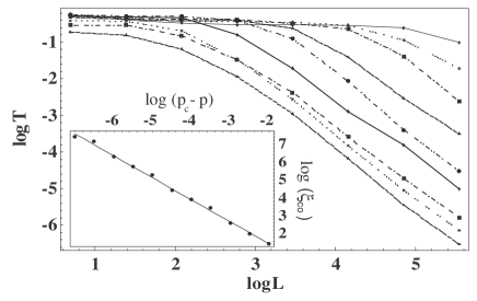
Figure 3: Crossover from the QH critical point to the MIT: transmission as a function of length (on a log-log scale) for different values of $(p_{c}-p)$ , demonstrating the crossover from the QH behavior (length-independent transmission) to a classical power-law dependence. Inset: The crossover length $\xi_{co}$ as a function of the $(p_{c}-p)$ on a log-log scale, with a slope $\nu=1.23$, close to the percolation correlation exponent.

All these observations have clear experimental relevance. As mentioned above, the QH to the MIT crossover has been investigated experimentally, but with no detailed investigation of the critical behavior. We thus predict that the critical exponent along this line will be the classical percolation exponent, $\nu_{p}$, and not the QH exponent, with two relevant length scales for any finite system. Similarly, one can experimentally investigate the quantum SIT to the classical superconductor - conductor transition, for different temperatures. The theory predicts that once the dephasing length becomes smaller than the system size (i.e. $q$ becomes nonzero), the critical behavior will correspond to classical percolation. Moreover, we predict that the conductance at the critical point will vary from its universal value at the quantum transition to a length dependence value according to Eq.(5).

Another result of the proposed phase diagram is the existence of an intermediate metallic regime in the QH and in the SITs. Imagine changing a physical parameter (e.g. density or magnetic field) along the broken line in Fig. 2. Then there is one transition from an insulator to a metal, and then from a metal to a QH liquid (or a superconductor), consistent with experimental observations for the QH transitionnoncritical and the SIT metallic . The critical behavior of both these transitions is determined by classical percolation. Thus the theory predicts that the QH critical behavior can only be observed in system where these transitions coalesce into a single transition. This can be tuned, for example, by lowering the temperature and changing the dephasing length. Thus the theory can explain the different exponents observed experimentally and predicts a crossover between the different critical behaviors as a function of temperature.

It should be noted that some aspects of this phase diagram are not dissimilar to the one presented in Ref.dissipation . Here, however, we do not invoke any zero temperature dissipation. Rather, if, as expected, the dephasing length diverges at $T\rightarrow 0$ (i.e. $q\rightarrow 0$) the theory predicts only two stable phases - the QH (or superconducting) phase and the Anderson insulator phase.

We would like to acknowledge fruitful discussions with A. Aharony and O. Entin-Wohlman. This research has been funded by the ISF.

References

- (1) B. Huckestein, Rev. Mod. Phys. 67, 357 (1995).
- (2) C.V.Mil‘nikov and I.M.Sokolov, Pizma Zh. Eksp. Teor. Fiz. 48, 494 (1988).
- (3) H. P. Wei et al., Phys. Rev. Lett. 61, 1294 (1988); S. Koch et al., Phys. Rev. Lett. 67, 883 (1991).
- (4) A. A. Shashkin et al., Phys. Rev. B 49, 14486 (1994); R. B. Dunford et al., Physica, B 289 496 (2001).
- (5) D. Shahar et al., Solid. State. Comm. 107,19; N. Q. Balaban et al., Phys. Rev. Lett. 81,4967 (1998).
- (6) P. Hopkins et al., Phys. Rev. B 39,12708 (1989); M. Hilke et al., Nature 395, 675 (1998).
- (7) L. P. Pryadko and A. Auerbach, Phys. Rev. Lett. 82, 1253 (1999).
- (8) D. B. Haviland, Y. Liu, and A. M. Goldman, Phys. Rev. Lett. 62 2180 (1989).
- (9) Y. Liu et al., Phys. Rev. Lett. 67 2068 (1991).
- (10) A. F. Hebard and M. A. Paalanen, Phys. Rev. Lett. 65, 927 (1990); A. Yazdani and A. Kapitulnik, Phys. Rev. Lett. 74, 3037 (1995); D. Ephron, et al., Phys. Rev. Lett. 76, 1529 (1996); N. Mason and A. Kapitulnik, Phys. Rev. Lett. 82, 5341 (1999).
- (11) E. Abrahams, S. V. Kravchenko and M. P. Sarachik, Rev. Mod. Phys. 90 251 (2001) and references therein.
- (12) Y. Meir, Phys. Rev. Lett. 83, 3506 (1999), and experimental references therein.
- (13) S. Das Sarma et al., cond-mat/0406655.
- (14) A. A. Shashkin et al., Phys. Rev. Lett. 73, 3141 (1994); I. V. Kukushkin et al., Phys. Rev. B 53, R13260 (1996).
- (15) D. Kowal and Z. Ovadyahu, Solid State Comm. 90, 783 (1994).
- (16) S. He and X. C. Xie, Phys. Rev. Lett. 80,3324 (1998).
- (17) E. Shmishoni, A. Auerbach and A. Kapitulnik, Phys. Rev. Lett. 80, 3352 (1998).
- (18) Y. Dubi, Y. Meir and Y. Avishai, cond-mat/0406008.
- (19) M. Buttiker, Phys. Rev. B 33, 3020 (1986); See also J. Shi, S. He and X. C. Xie, cond-mat/9904393 .
- (20) D. P. Arovas, M. Janssen and B. Shapiro, Phys. Rev. B 56, 4751 (1997); A. G. Galstyan and M. E. Raikh, Phys. Rev. B 56, 1442 (1997); Y. Avishai, Y. Band and D. Brown, Phys. Rev. B 60, 8992 (1999) .
- (21) E. Shimshoni, cond-mat/0406703.
- (22) Y. Hanein et al., Nature 400, 735 (1999).
- (23) A. Kapitulnik et al., Phys. Rev. B 63, 125322 (2001).