Asymmetric simple exclusion processes with diffusive bottlenecks

Abstract

One-dimensional asymmetric simple exclusion processes (ASEPs) which are coupled to external reservoirs via diffusive transport are studied. These ASEPs consist of active compartments characterized by directed movements of the particles and diffusive compartments in which the particles undergo unbiased diffusion. Phase diagrams are obtained by a self-consistent mean field approach and by Monte Carlo simulations. The diffusive compartments act as diffusive bottlenecks if the velocity of the driven compartments or ASEPs is sufficiently large. A diffusive bottleneck at the boundary of the system leads to the absence of a maximal current phase, while a diffusive bottleneck in the interior of the system leads to a new phase characterized by different densities in the two active compartments adjacent to the diffusive one and to a maximal current defined by the bottleneck.

I Introduction

Asymmetric simple exclusion processes (ASEPs) are simple one-dimensional driven lattice gases with hard core exclusion. They were originally introduced in the context of protein synthesis MacDonald et al. (1968) and have attracted much interest during the last years as simple models for boundary-induced phase transitions Krug (1991), for which many rigorous results have been obtained Derrida et al. (1992); Schütz and Domany (1993); Derrida et al. (1993). In the open system, different stationary states are found, which depend on the rates of injection and extraction of particles at the ends. Varying the injection and extraction rates, or equivalently the densities at the left and right boundary, both continuous and discontinuous phase transitions are observed. The actual stationary state is selected via the dynamics of domain walls and density fluctuations Kolomeisky et al. (1998).

Promising candidates for the experimental observation of these phase transitions are systems of cytoskeletal motors which move unidirectionally along cytoskeletal filaments Lipowsky et al. (2001); Nieuwenhuizen et al. (2002); Klumpp and Lipowsky (2003). However, these motors unbind from their track after a few seconds, since their binding energy can be overcome by thermal fluctuations. Observed over sufficiently long times which exceed a few seconds, they alternate between the bound and the unbound state and perform peculiar random walks. If a motor is bound to a filament, it moves in a directed way along the filament, while unbound motors diffuse freely. As motors are strongly attracted by the filament, the motor density along the filament can be large even if the overall motor concentration is rather small, which implies that hard core exclusion plays an important role in the bound state. To study these combined movements, we have recently introduced a class of lattice models where bound and unbound motor movements are described as biased and symmetric random walks on a lattice, respectively Lipowsky et al. (2001); Nieuwenhuizen et al. (2002); Klumpp and Lipowsky (2003). In these models, the traffic of motors along a filament is an asymmetric simple exclusion process with the additional property that motors can attach to and detach from the track.

For open tube systems with a single filament and fixed motor concentrations at the tube ends, the same types of phases are found as for the usual one-dimensional ASEP Klumpp and Lipowsky (2003). If the filament is shorter than the tube and motors have to diffuse over a certain distance to reach one end of the filament from the left boundary and again to reach the right boundary from the other end of the filament, the phase boundaries of the system can be shifted by changing geometrical tube parameters or motor parameters. In particular, a maximal current phase, in which the current attains its maximally possible value, can only be found if the diffusive currents from the left end of the tube to the filament and from the filament to the right end of the tube can be as large as this maximal current. These diffusive currents however are restricted by the diffusion coefficient of the unbound motors and by geometric parameters Klumpp and Lipowsky (2003).

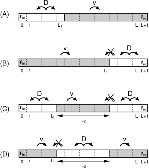
Figure 1: Four geometries of one-dimensional lattices which consist of active compartments (gray) where transport is described by an asymmetric simple exclusion process and diffusive compartments (white) where transport is described by a symmetric exclusion process. The linear extensions of the compartments are denoted by $L_{1}$, $L_{2}$, and $L_{3}$. The total length of the system is given by $L=L_{1}+L_{2}$ in cases (A) and (B) and by $L=L_{1}+L_{2}+L_{3}$ in cases (C) and (D). In the active compartments, motion is completely biased and particles hop to the right with probability $v$, while in the diffusive compartments, particles hop both to the left and to the right with probability $D$. In addition, we do not allow particles to enter the active compartments from the right. The densities at the boundary sites $x=0$ and $x=L+1$ are fixed to $\rho_{\rm in}$ and $\rho_{\rm ex}$, respectively.

The latter phenomenon is generic and not restricted to the specific tube geometry. In the following, we study several one-dimensional systems which consist of compartments characterized by active or diffusive transport. We will discuss four simple geometries as shown schematically in Fig. 1. While particles move only to the right in the active compartments, forward and backward steps occur with the same probability in the diffusive compartments. For these models, we determine the phase diagram analytically using a mean field approach to calculate effective boundary densities or effective injection and extraction rates for the active compartments. The method is based on the constraint that the stationary current must be equal in all compartments.

The article is organized as follows. After introducing the model in section II, we discuss diffusive injection and extraction of particles into/from an active compartment in section III. We start with only diffusive injection in section III.1 which corresponds to case (A) in Fig. 1, proceed with only diffusive extraction in section III.2, see case (B) in Fig. 1, and then study the case (C), for which particles are both injected and extracted via diffusive compartments, see section III.3. We compare the mean field results with Monte Carlo simulation in section III.4. Finally, we discuss the case of a diffusive compartment between two active compartments as shown as case (D) in Fig. 1 in section IV. This case corresponds to a defect that must be overcome by unbiased diffusion.

II The model

In the following, we will discuss transport on one-dimensional lattices. The coordinate along the lattice is denoted by $x$ and will be measured in units of the lattice constant $\ell$.

We consider systems that can be decomposed into two or three different compartments in which transport is either diffusive or directed. The four cases that will be discussed in the following are shown schematically in Fig. 1. The total length of the system is taken to be $L$ in all cases. The linear extensions of the compartments are denoted by $L_{1}$, $L_{2}$, and $L_{3}$, compare Fig. 1. In case (A), the system consists of a left compartment with $1\leq x<L_{1}$, where transport is diffusive, and a right compartment with $L_{1}+1\leq x\leq L_{1}+L_{2}=L$, where transport is active or directed. In case (B), transport is directed in the left compartment and diffusive in the right compartment. The cases (C) and (D) correspond to situations where the systems consist of three compartments with $L=L_{1}+L_{2}+L_{3}$. In case (C), transport is driven in the middle compartment with $L_{1}+1\leq x\leq L_{1}+L_{2}$ and diffusive in the left and right ones. Finally in case (D), transport is directed in two compartments, the left and the right one, but diffusive in the middle compartment. In all cases, we will assume that the extensions of the active compartments are sufficiently large, so that we can neglect finite-size effects.

In the following, we will take the active transport to be always directed to the right and to be totally asymmetric, i.e., we do not allow backward steps in the compartments with active transport. At lattice sites which belong to such an active compartment, particles attempt to hop to the adjacent lattice site to their right with a certain probability per unit time $\tau$. We denote this probability by $v$ since it is equal to the velocity of a particle in the active compartment (and in the absence of other particles), measured in units of $\ell/\tau$. The hopping attempt is rejected if the target site is already occupied by another particle. In summary, motion in the active compartment is described by a totally asymmetric simple exclusion process.

In contrast, motion in the diffusive compartments is described by a symmetric exclusion process. A particle at a lattice site which belongs to a diffusive compartment attempts to make a forward and a backward step with equal probability $D$, which corresponds to the diffusion coefficient measured in units of $\ell^{2}/\tau$. Note that we could eliminate one parameter by measuring time in units of the time scale for diffusive steps of size $\ell$ by choosing $\tau=\ell/(2D)$ (for this choice, the diffusion coefficient measured in units of $\ell^{2}/\tau$ would be given by $D=1/2$). This implies that the results which we derive in the following will depend only on the ratio $v/D$. All hopping attempts in the diffusive compartments are again rejected if the target site is occupied by another particle. In order to simplify the following calculations, we do not allow particles to enter the active compartments from the right, i.e. all hopping attempts from the first site of a diffusive compartment to the last site of the active compartment to its right — from $L_{1}+1$ to $L_{1}$ in case (B) and (D) and from $L_{1}+L_{2}+1$ to $L_{1}+L_{2}$ in case (C) — are rejected.

Finally, the densities at the boundary sites $x=0$ and $x=L+1$ have the fixed values

$$\rho(x=0)=\rho_{\rm in}\qquad{\rm and}\qquad\rho(x=L+1)=\rho_{\rm ex}.$$ (1)

These sites are taken to have the same dynamics as the adjacent compartments of the system. Particles thus attempt to enter the system from the left with probability $D\rho_{\rm in}$ if the first compartment is diffusive and with probability $v\rho_{\rm in}$ if it is an active compartment. Particles at the last lattice site with $x=L$ leave the system to the right with probability $v(1-\rho_{\rm ex})$ if the site $x=L$ belongs to an active compartment and with probability $D(1-\rho_{\rm ex})$ if it belongs to a diffusive one. In the latter case, particles also try to enter the system from the right at $x=L$ with probability $D\rho_{\rm ex}$. Likewise, particles at site $x=1$ can leave the system with probability $D(1-\rho_{\rm in})$ if $x=1$ belongs to a diffusive compartment. As before, particles can only enter the system at $x=1$ or $x=L$ if these sites are not occupied.

III Diffusive injection and extraction of particles

In this section, we consider the cases (A)–(C), where transport is driven or active in one compartment, but particles are diffusively injected and/or extracted from the system and have to diffuse over a certain distance before they reach the active compartment and/or before they can leave the system at the right end.

As mentioned before, the active compartment is described by an asymmetric simple exclusion process. Let us therefore briefly summarize what is known about the phase diagram of this process, see, e.g., Ref. Kolomeisky et al. (1998). In an open system, where the densities are fixed to $\rho_{\rm in}$ and $\rho_{\rm ex}$ at the left and right boundary of the ASEP, respectively, the stationary state is determined by the boundary densities. The stationary states are characterized by the bulk density $\rho^{0}$ and the stationary current $J$.

For the ASEP with open boundaries, three different phases can be distinguished as shown in Fig. 2: If the density at the left boundary is relatively small and satisfies $\rho_{\rm in}<1/2$ and $\rho_{\rm in}<1-\rho_{\rm ex}$, the system is in the low density phase (LD) for which the bulk density is equal to the left boundary density and the current is $J=v\rho_{\rm in}(1-\rho_{\rm in})$. If the density at the right boundary is relatively large with $\rho_{\rm ex}>1/2$ and $\rho_{\rm ex}>1-\rho_{\rm in}$, the system is in the high density phase (HD), the bulk density is equal to the right boundary density, and the current is $J=v\rho_{\rm ex}(1-\rho_{\rm ex})$. At the transition from the low density to the high density phase, the current is continuous, but the bulk density is discontinuous. Finally, for $\rho_{\rm in}>1/2$ and $\rho_{\rm ex}<1/2$, the system is in the maximal current phase, where the current is maximal, $J=v/4$ and the bulk density is $1/2$. The transitions to the maximal current phase are continuous.

In contrast to the simple ASEPs just described, our systems are characterized by the property that at least one of the boundary densities of the active compartments is not fixed, but adjusted by the dynamics of the system. In the following, we will determine the phase diagrams of these systems using a mean field approach. We proceed in three steps and consider first diffusive injection and extraction of particles separately, combining them in the last step.

III.1 Diffusive injection of particles

First we consider case (A), a system with only diffusive injection of particles. Particles leave the system at the right boundary with rate $v(1-\rho_{\rm ex})$ and no particles enter the system at the right end. In the stationary state, the current $J$ must be the same in both compartments. In the left compartment with $1\leq x\leq L_{1}$ where transport is diffusive, the density is then given by $\rho(x)=\rho_{\rm in}-xJ/D$. Within mean field approximation, the right compartment with $L_{1}+1\leq x\leq L$, corresponds to the usual ASEP with the effective left boundary density

$$\rho_{\rm in,eff}=\frac{D\rho(L_{1})}{v}=\frac{D\rho_{\rm in}}{v}-\frac{L_{1}J}{v}.$$ (2)

as follows from $v\rho_{\rm in,eff}\equiv D\rho(L_{1})$. The quantity $v\rho_{\rm in,eff}$ corresponds to the rate with which particles attempt to enter the ASEP at its left boundary. Note that (i) this effective boundary density depends on the current $J$ and (ii) that $\rho_{\rm in,eff}$ can be larger than one. The right boundary density is given by $\rho_{\rm ex}$.

The phase diagram can now be determined in a self-consistent way. As in the tube system studied in Ref. Klumpp and Lipowsky (2003), the same phases are found as for the one-dimensional ASEP, but the location of the transition lines depends on the values of the model parameters $v/D$ and $L_{1}$, and the maximal current phase may be shifted out of the physically accessible range of the parameters.

The system is in the maximal current phase if $\rho_{\rm ex}<1/2$ and $\rho_{\rm in,eff}>1/2$. In this case the current is $J=v/4$, and the condition

$$\rho_{\rm in,eff}=\frac{D}{v}\rho_{\rm in}-\frac{L_{1}}{4}\geq\frac{1}{2}$$ (3)

implies that the system is in the maximal current phase for

$$\rho_{\rm in}\geq\frac{v}{2D}\left(1+\frac{L_{1}}{2}\right).$$ (4)

For large $v/D$, the latter value of the left boudary density is larger than one and therefore not physically accessible. This implies that a maximal current phase is only present for small velocities with $v/D<2/(1+L_{1}/2)$. If the velocity is larger, unphysically high densities would be necessary at the left boundary in order to establish a sufficiently large density gradient which could generate a diffusive current with the value $v/4$, the maximal current defined by the driven compartment. In this situation, the diffusive compartments acts as a diffusive bottleneck: If the maximally possible diffusive current through the diffusive compartment is smaller than $v/4$, a maximal current phase cannot occur, because the diffusive compartment cannot maintain the maximal current.

A simpler estimate comparing the maximal diffusive current $D/L_{1}$, which is restricted by the maximal density difference of one, with the maximal driven current $v/4$ yields the condition, $v/D<4/L_{1}$, which agrees with the previous one for large $L_{1}$, but is less restrictive for small $L_{1}$. The latter discrepancy reflects the fact that the maximal density difference in the diffusive compartment is actually smaller than one since the density at $x=L_{1}$ must be larger than zero.

In addition, a low density phase is found for $\rho_{\rm in,eff}<1/2$ and $\rho_{\rm in,eff}<1-\rho_{\rm ex}$ and a high density phase for $\rho_{\rm in,eff}>1-\rho_{\rm ex}$ and $\rho_{\rm ex}>1/2$. Along the transition line between the high density and low density phases we can use $J=v\rho_{\rm ex}(1-\rho_{\rm ex})$ and obtain

$$\rho_{\rm in}=\frac{v}{D}\left[1+(L_{1}-1)\rho_{\rm ex}-L_{1}\rho_{\rm ex}^{2}\right]$$ (5)

for the transition line between the low density and the high density phase. This line extends from the right upper corner of the phase diagram to the right upper corner of the maximal current phase region. If there is no maximal current phase, it ends at a point with $\rho_{\rm in}=1$ and $\rho_{\rm ex}>1/2$.

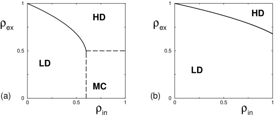
Figure 3: Phase diagrams for the ASEP with diffusive injection of particles at the left boundary, i.e. for case (A) as shown in Fig. 1, as a function of the left and right boundary densities $\rho_{\rm in}$ and $\rho_{\rm ex}$. The parameters are (a) $v=0.1$, $D=1/2$, and $L_{1}=10$; and (b) $v=0.2$, $D=1/2$, and $L_{1}=10$.

Phase diagrams for two cases are shown in Fig. 3. We have chosen $L_{1}=10$ and $D=1/2$ in both cases. The condition for the presence of a maximal current phase is then $v<1/6$. In Fig. 3(a), the velocity is $v=0.1<1/6$ and all three phases are present, while in Fig. 3(b), $v=0.2>1/6$ and the maximal current phase is absent. In the latter case the largest part of the phase diagram is covered by the low density phase.

In the maximal current phase the current is $J=v/4$. In the high density phase, it is determined by the right boundary density $\rho_{\rm ex}$ and has the value $J=v\rho_{\rm ex}(1-\rho_{\rm ex})$. Finally in the low density phase, the current is given by the self-consistency condition

$$J=v\rho_{\rm in,eff}(J)[1-\rho_{\rm in,eff}(J)],$$ (6)

which leads to a quadratic equation for the current. The solutions is uniquely determined by the limits $J=0$ for $\rho_{\rm in}=0$ and $J=v/4$ for $\rho_{\rm in}=\frac{v}{2D}(1+L_{1}/2)$ and is given by

$$J=\frac{v}{2L_{1}^{2}}\left(-1-L_{1}+2\frac{D}{v}L_{1}\rho_{\rm in}+\sqrt{\left(1+L_{1}-2\frac{D}{v}L_{1}\rho_{\rm in}\right)^{2}+4\frac{D}{v}L_{1}^{2}\rho_{\rm in}\left(1-\frac{D}{v}\rho_{\rm in}\right)}\right).$$ (7)

III.2 Diffusive extraction of particles

Next we consider case (B), in which particles which reach the end of the active compartment have to diffuse over a distance $L_{2}$ before they can leave the system at the right end. This case can be treated in the same way as the one with diffusive injection. Note, however, that it cannot simply be derived from the the latter one using particle-hole symmetry, because a particle at the site left of the driven compartment attempts to enter it with rate $D$, while a hole at the site right of the driven compartment does so with rate $v$.

The density profile in the diffusive compartment is given by $\rho(x)=\rho_{\rm ex}+(L+1-x)J/D$ for $L_{1}+1\leq x\leq L_{1}+L_{2}=L$. Therefore the effective rate with which particles attempt to leave the active compartment at $x=L_{1}$ is $v(1-\rho_{\rm ex}-L_{2}J/D)\equiv v(1-\rho_{\rm ex,eff})$ corresponding to an effective right boundary density of the driven compartment given by

$$\rho_{\rm ex,eff}=\rho_{\rm ex}+L_{2}J/D.$$ (8)

The maximal current phase is now found for $\rho_{\rm in}>1/2$ and

$$\rho_{\rm ex}<\frac{1}{2}-\frac{L_{2}v}{4D},$$ (9)

which is always $\leq 1/2$. Again the maximal current phase is only present if the range of boundary densities defined by Eq. (9) is physically accessible. Here the corresponding condition is $\rho_{\rm ex}>0$, which is valid for $v/D<2/L_{2}$. The latter condition expresses again the fact that the diffusive compartment must also support this maximal current. The diffusive current is, however, restricted by the maximally possible value of the density gradient in the right (diffusive) compartment, $1/(2L_{2})$, which leads to a maximal diffusive current of $D/(2L_{2})$. If the latter current is smaller than $v/4$, a stationary maximal current phase is absent; therefore, the presence of the maximal current phase requires that the maximal diffusive current is $\geq v/4$ which leads to the condition $v/D<2/L_{2}$.

The condition $1-\rho_{\rm ex,eff}=\rho_{\rm in}$ with $J=v\rho_{\rm in}(1-\rho_{\rm in})$ yields the transition line between the low density and the high density phase

$$\rho_{\rm ex}=1-\rho_{\rm in}(1+\frac{v}{D}L_{2})+\frac{v}{D}L_{2}\rho_{\rm in}^{2}.$$ (10)

For velocities larger than $2D/L_{2}$, which is the maximal value for the occurrence of a maximal current phase, this line ends at a point in the phase diagram with $\rho_{\rm in}=0$ and $\rho_{\rm ex}<1/2$. In this case the high density phase covers most of the phase diagram.

The current is $J=v/4$ in the maximal current phase and $J=v\rho_{\rm in}(1-\rho_{\rm in})$ in the low density phase. In the high density phase, it is again given by a self-consistency condition $J=v\rho_{\rm ex,eff}(1-\rho_{\rm ex,eff})$, where $\rho_{\rm ex,eff}$ is a function of $J$, from which we obtain

$$J=\frac{v}{2(L_{2}v/D)^{2}}\left(-1+\frac{v}{D}L_{2}(1-2\rho_{\rm ex})+\sqrt{1-2\frac{v}{D}L_{2}+4\frac{v}{D}L_{2}\rho_{\rm ex}+\left(\frac{v}{D}L_{2}\right)^{2}}\right).$$ (11)

III.3 Both diffusive injection and extraction of particles

Now we consider case (C), i.e., we combine the two preceding cases. Transport is now driven in the middle compartment for which we have the effective boundary densities

$$\rho_{\rm in,eff}=\frac{D\rho_{\rm in}}{v}-\frac{L_{1}J}{v}\qquad{\rm and}\qquad\rho_{\rm ex,eff}=\rho_{\rm ex}+L_{3}J/D.$$ (12)

The phase boundary between the low density phase and the maximal current phase is not affected by adding another compartment at the right end, thus we can use the result from case (A). Likewise the phase boundary between the high density phase and the maximal current phase is unaffected by the left diffusive compartment, so that we can use the result from case (B) upon substituting $L_{2}$ with $L_{3}$. The maximal current phase is therefore found for

$$\rho_{\rm in}>\frac{v}{2D}\left(1+\frac{L_{1}}{2}\right)\quad{\rm and}\quad\rho_{\rm ex}<\frac{1}{2}-\frac{L_{3}v}{4D}.$$ (13)

It is present if $v/D<2/(1+L_{1}/2)$ and $v/D<2/L_{3}$. In addition, the current is given by Eqs. (7) and (11) in the low density and the high density phase, respectively.

Finally, the transition line between these two phases is obtained from the condition $\rho_{\rm in,eff}=1-\rho_{\rm ex,eff}$, which leads to

$$\rho_{\rm in}=\frac{v}{D}\left[1-\rho_{\rm ex}+\frac{J(\rho_{\rm ex})}{v}(L_{1}-\frac{v}{D}L_{3})\right],$$ (14)

where $J(\rho_{\rm ex})$ is the current in the high density phase for the right boundary density $\rho_{\rm ex}$ as given by Eq. (11). The complete phase diagram is shown in Fig. 4, where we have chosen parameters for which a maximal current phase is present.

III.4 Comparison with simulations

In addition to the self-consistency calculations presented above, we performed Monte Carlo simulations. In this section, we compare the simulation results with the mean field predictions for case (C).

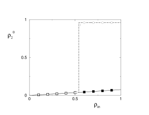
Figure 5: Bulk density $\rho_{2}^{0}$ in the active compartment of a system with geometry (C) as a function of the left boundary density $\rho_{\rm in}$. Lines are the mean field results and symbols are simulation data. The right boundary density is fixed to $\rho_{\rm ex}=0$ (solid line) and $\rho_{\rm ex}=0.5$ (dashed line). Parameters have been chosen so that no maximal current phase is found; $v=1$, $D=1/2$, $L_{1}=L_{3}=6$ and $L_{2}=388$.

In the case where the maximal current phase is absent, i.e. for large velocities, we find quantitative agreement of the measured current and bulk density with the predictions of the mean field calculation. The transition from the low density to the high density phase occurs at the predicted density. As an example, we show results for the bulk density $\rho_{2}^{0}$ in the active compartments in Fig. 5, where we have chosen $\rho_{\rm ex}=0$ and $\rho_{\rm ex}=0.5$. In the first case, the system is in the low density phase for all values of $\rho_{\rm in}$, in the second case, a transition to the high density phase is found at $\rho_{\rm in}\simeq 0.54$. The mean field results (lines) and the simulation data (symbols) agree well.

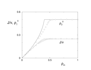
Figure 6: Current $J$ (dashed line) and bulk density $\rho_{2}^{0}$ (solid line) in the active compartment of a system with geometry (C) as a function of the left boundary density $\rho_{\rm in}$ for a case with transition to the maximal current phase. The lines are the predictions of the mean field calculation, the symbols simulation data. The parameters are $v=0.1$, $D=1/2$, $L_{1}=L_{3}=6$, $L_{2}=388$, and $\rho_{\rm ex}=0$.

If a maximal current phase is present, i.e. for small velocities, the agreement is less good, although the phase diagram is still in qualitative agreement with the mean field predictions. Fig. 6 shows again results for the case $\rho_{\rm ex}=0$. Close to the transition to the maximal current phase the current is smaller than predicted by the mean field calculation. Therefore the transition to the maximal current phase is shifted towards a larger value of $\rho_{\rm in}$ and the increase of the bulk density near the transition is less steep. Far from the transition, however, agreement is again good. Likewise, the transition line between the low density and the high density phase is also shifted towards larger $\rho_{\rm in}$, as this transition line ends on the phase boundary of the maximal current phase. Agreement becomes again better far from the maximal current phase, since the other end point of the line ($\rho_{\rm in}=0$, $\rho_{\rm ex}=1$) is exact.

IV Diffusive bottleneck in the middle

Finally, let us consider case (D), where active transport is interrupted by a diffusive compartment. In the case of molecular motors, this can be realized by a gap in the filament network, along which active transport takes place. Motors thus have to overcome this gap by diffusion before they can rebind to a filament and continue their active movements. If the middle compartment consists of only one lattice site, $L_{2}=1$, this system reduces to the case of an ASEP with a single defect which has been discussed previously, see Refs. Janowsky and Lebowitz (1992); Kolomeisky (1998).

The effective right boundary density for the left active compartment is

$$\rho_{\rm ex,eff}=\rho(L_{1}+1)$$ (15)

and the effective left boundary density for the right active compartment is

$$\rho_{\rm in,eff}=\frac{D\rho(L_{1}+L_{2})}{v}=\frac{D\rho(L_{1}+1)-(L_{2}-1)J}{v}.$$ (16)

In this case, there are five possible phases. Because the current is the same in both active compartments, the bulk densities in the left and right compartment, $\rho_{1}^{0}$ and $\rho_{3}^{0}$, respectively, are either equal or related by $\rho_{1}^{0}=1-\rho_{3}^{0}$. If the bulk densities in both active compartments are equal, $\rho_{1}^{0}=\rho_{3}^{0}$, there are three possibilities. Both compartments can be in the low density, high density or maximal current phase. We denote these three cases by LD–LD, HD–HD, and MC–MC, respectively. If the densities are not equal, we have $\rho_{1}^{0}=1-\rho_{3}^{0}$, and there are two additional possible phases, where one compartment is in the high density and the other in the low density phase. These phases will be denoted by HD–LD and LD–HD if $\rho_{1}^{0}$ is larger or smaller than $\rho_{3}^{0}$, respectively.

IV.1 Phases with equal densities in the active compartments

In the MC–MC phase, the current is $J=v/4$ and we have four conditions for the boundary densities, $\rho_{\rm in}>1/2$, $\rho_{\rm ex}<1/2$, $\rho_{\rm in,eff}>1/2$ and $\rho_{\rm ex,eff}<1/2$. The first two conditions are the same as for an ASEP without the diffusive compartment and the latter two conditions yield $v/D<2/(1+L_{2})$. The maximal current phase is found only for small velocities, for larger velocities in the active compartments, the diffusive section acts again as a diffusive bottleneck.

The LD–LD phase is characterized by $J=v\rho_{\rm in}(1-\rho_{\rm in})=v\rho_{\rm in,eff}(1-\rho_{\rm in,eff})$. As both $\rho_{\rm in}$ and $\rho_{\rm in,eff}$ must be smaller than $1/2$, this implies $\rho_{\rm in}=\rho_{\rm in,eff}$. Together with the condition $\rho_{\rm ex}<1-\rho_{\rm in,eff}$ for the right active compartment, this implies that the LD–LD phase is found within the region of the phase diagram where the low density phase of the usual ASEP is located. An additional condition is given by $\rho_{\rm ex,eff}=\rho(L_{1}+1)<1-\rho_{\rm in}$. Thus, with the condition $\rho_{\rm in}=\rho_{\rm in,eff}$, we obtain $\rho(L_{1}+1)$ as a function of $\rho_{\rm in}$,

$$\rho(L_{1}+1)=\frac{v}{D}[\rho_{\rm in}+(L_{2}-1)\rho_{\rm in}(1-\rho_{\rm in})]$$ (17)

which leads to the inequality

$$\frac{v}{D}[\rho_{\rm in}+(L_{2}-1)\rho_{\rm in}(1-\rho_{\rm in})]+\rho_{\rm in}<1.$$ (18)

Because $\rho_{\rm in}<1/2$, the left hand side of this inequality is increasing monotonically and the solution is given by $\rho_{\rm in}<\rho_{\rm in,*}$, where $\rho_{\rm in,*}$ is the solution of the equation which is obtained upon substituting ’$<$’ with ’$=$’ in Eq. (18). This solution is uniquely determined by the limiting case $L_{2}=1$, in which Eq. (18) yields $\rho_{\rm in}<1/(1+v/D)$. As a result we obtain the condition

$$\rho_{\rm in}<\rho_{\rm in,*}\equiv\frac{\frac{v}{D}L_{2}+1-\sqrt{(\frac{v}{D}L_{2}+1)^{2}-4\frac{v}{D}(L_{2}-1)}}{2\frac{v}{D}(L_{2}-1)}.$$ (19)

If $\rho_{\rm in,*}$ is larger than $1/2$, this condition does not further restrict the occurrence of the LD–LD phase, since for $\rho_{\rm in}=1/2$ the transition to the maximal current phase takes place. Indeed, $\rho_{\rm in,*}>1/2$ implies the simpler condition $v/D<2/(L_{2}+1)$, which is exactly the condition we derived above as a condition for the presence of the MC–MC phase.

On the other hand, if $\rho_{\rm in,*}<1/2$, condition (18) yields a restriction of the LD–LD phase to the region in the phase diagram with $\rho_{\rm in}<\rho_{\rm in,*}$. Therefore we conclude that for large velocities with $v/D>2/(L_{2}+1)$, the transition to the MC–MC phase at $\rho_{\rm in}=1/2$ is replaced by a transition to another phase at $\rho_{\rm in}=\rho_{\rm in,*}$. The only possibility for this phase is the HD–LD phase which will be discussed below.

Finally note that for $L_{2}=1$ our result recovers the condition for the ASEP with a defect Kolomeisky (1998), where for $v/D<1$ the phase diagram is the same as without the defect, while for $v/D>1$ a phase dominated by the defect is found.

The HD–HD phase can be treated in the same way and gives corresponding results. A HD–HD phase can be found for $\rho_{\rm ex}>1-\rho_{\rm in}$ and $\rho_{\rm ex}>1/2$ for small velocities which fulfill again the condition $v/D<2/(L_{2}+1)$, while for larger velocities an additional restricting condition is found, namely $\rho_{\rm ex}>\rho_{\rm ex,*}$ with $\rho_{\rm ex,*}\equiv 1-\rho_{\rm in,*}$.

IV.2 Phases with different densities in the active compartments

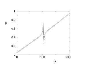
Figure 7: Density profile for the ’LD–HD’ phase or coexistence of the LD–LD and HD–HD phases for a system with a diffusive defect [case (D)]. As discussed in the text, the profile is essentially linear rather than consisting of two plateaus. The parameters are $v=1$, $D=1/2$, $L=205$, $L_{1}=L_{3}=101$, $L_{2}=3$, $\rho_{\rm in}=0.05$, and $\rho_{\rm ex}=0.95$.

For an LD–HD phase, the current must be $J=v\rho_{\rm in}(1-\rho_{\rm in})=v\rho_{\rm ex}(1-\rho_{\rm ex})$. This implies that the densities are $\rho_{\rm in}=1-\rho_{\rm ex}$, i.e., a stationary state with a low density in the left, but a high density in the right active compartment can only be expected along the line, where the low density and high density phases coexist in the ASEP without a diffusive compartment. In this case, however, a domain wall diffuses through the system in the usual ASEP resulting in a density profile which increases linearly Kolomeisky et al. (1998). The same can be expected for our case with the exception of the regions close to the diffusive compartment. This behavior has previously been observed in simulations for the case of an ASEP with a defect Kolomeisky (1998) which correspond to our case with $L_{2}=1$ and we find the same behavior in Monte Carlo simulations for larger $L_{2}$, see Fig. 7.

Finally, let us consider the possibility of a HD–LD phase. In this case the current is $J=v\rho_{\rm in,eff}(1-\rho_{\rm in,eff})=v\rho_{\rm ex,eff}(1-\rho_{\rm ex,eff})$ which, together with the conditions $\rho_{\rm in,eff}<1/2$ and $\rho_{\rm ex,eff}>1/2$, implies $\rho_{\rm in,eff}=1-\rho_{\rm ex,eff}$. Substituting the expression for the effective boundary densities, we obtain a quadratic equation for $\rho(L_{1}+1)$ with the solution

$$\rho(L_{1}+1)=\rho_{\rm ex,*}=1-\rho_{\rm in,*}$$ (20)

with $\rho_{\rm in,*}$ as given by Eq. (19). For $L_{2}=1$ we recover again the corresponding result for the ASEP with a defect.

IV.3 Phase diagrams

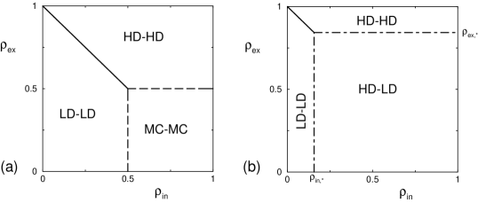
Figure 8: Phase diagrams for case (D), i.e. for a diffusive compartment between two active compartments, as a function of the left and right boundary density, $\rho_{\rm in}$ and $\rho_{\rm ex}$. (a) Small velocity, $v=0.1$ and (b) large velocity, $v=1$. The diffusive section has length $L_{2}=3$ and the diffusion coefficient is $D=1/2$.

We can now summarize the results into phase diagrams as shown in Fig. 8. There are two different cases: If $v/D<2/(1+L_{2})$, the phase diagram corresponds to the one of the ASEP without the diffusive compartment, see Fig. 8(a). The bulk density is equal in both active compartments. If, on the other hand, the velocity is larger with $v/D>2/(1+L_{2})$, the diffusive compartment acts as a bottleneck and the phase diagram is modified, see Fig. 8(b). We find the LD–LD phase for $\rho_{\rm in}<\rho_{\rm in,*}$ and $\rho_{\rm in}<1-\rho_{\rm ex}$ and the HD–HD phase for $\rho_{\rm ex}>\rho_{\rm ex,*}$ and $\rho_{\rm ex}>1-\rho_{\rm in}$. For $\rho_{\rm in}>\rho_{\rm in,*}$ and $\rho_{\rm ex}<\rho_{\rm ex,*}$, the system exhibits the HD–LD phase. While in the LD–LD and HD–HD phases, the bulk densities in the active compartments and the current are determined by the boundary densities, these quantities are independent of the boundary densities in the HD–LD phase and depend only on the ratio $v/D$ and the length $L_{2}$ of the diffusive compartment.

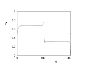
Figure 9: Density profile for the HD–LD phase in case (D) with $\rho_{\rm in}=0.5$, $\rho_{\rm ex}=0$, $v=0.25$, and $D=1/2$. The geometrical parameters are as in Fig. 7.

The HD–LD phase has some similarities to a maximal current phase. The current is constant throughout this phase and attains its maximal value compared to all other phases, $J=v\rho_{\rm in,*}(1-\rho_{\rm in,*})=v\rho_{\rm ex,*}(1-\rho_{\rm ex,*})$. This maximal value, however, is not determined by the active compartments, but corresponds to the maximal current which can be supported by the diffusive compartment. Correspondingly, the density profiles in the HD–LD phase (shown in Fig. 9) do not exhibit the power-law behavior known from the usual maximal current phase. The bulk densities in the left and right active compartments are constant in this phase as well and are given by $\rho_{\rm ex,*}$ and $\rho_{\rm in,*}$, respectively. Note, however, the following difference compared to the usual maximal current phase. The transitions to the maximal current phase in the usual ASEP are continuous. The transitions to the HD–LD phase in our case are somewhat peculiar in the sense that they are continuous in one compartment, but discontinuous in the other. For example, at the transition from the LD–LD phase to the HD–LD phase, the density $\rho_{3}^{0}$ in the right active compartment is continuous, but the bulk density $\rho_{1}^{0}$ in the left active compartment exhibits a jump from $\rho_{\rm in,*}$ to $1-\rho_{\rm in,*}$.

We performed again Monte Carlo simulations and compared the results with the mean field predictions. As a result, we find that the phase diagram obtained by the self-consistent mean field approach is recovered for small velocities. For large velocities, on the other hand, the qualitative behavior is correctly predicted by the mean field calculation, but the transition lines for the transition to the HD–LD phase are shifted. For example for $v=1$, $D=1/2$, and $L_{2}=3$, we find the transition from the LD–LD phase to the HD–LD phase at $\rho_{\rm in}\simeq 0.08$ in the simulations, while our mean field calculation predicts a transition at $\rho_{\rm in}=\rho_{\rm in,*}\simeq 0.13$. Correspondingly, there are also differences in the values for the current in the HD–LD phase and the critical value of the velocity is found to be smaller than predicted by the mean field calculation. For $L_{2}=3$ and $D=1/2$, we observe the usual maximal current phase for $v\mathrel{\mathchoice{\vbox{\offinterlineskip\halign{\hfil$\displaystyle#$\hfil\cr<\cr\sim\cr}}}{\vbox{\offinterlineskip\halign{\hfil$\textstyle#$\hfil\cr<\cr\sim\cr}}}{\vbox{\offinterlineskip\halign{\hfil$\scriptstyle#$\hfil\cr<\cr\sim\cr}}}{\vbox{\offinterlineskip\halign{\hfil$\scriptscriptstyle#$\hfil\cr<\cr\sim\cr}}}}0.15$ in the simulations while the mean field approach yields $v<0.25$.

Finally, let us add a remark concerning the density profiles in the HD–LD phase. From our mean field approach, we expect the constant bulk densities in the left and right active compartments to be approached exponentially from the left and right boundary, respectively. This is the case in the simulation data; however, in addition, an excess density close to the diffusive compartment is observed, which is not expected from the mean field approach, see Fig. 9. As reported previously for the case of an ASEP with a single defect site Janowsky and Lebowitz (1992), this excess density decays as a power-law $\sim x^{-1}$, so that some kind of long-range order is also present in this phase which plays the role of a maximal current phase for the system with a diffusive bottleneck.

V Summary and conclusions

We have discussed transport in one-dimensional lattices which consist of two or three compartments where transport is either driven or diffusive, a situation that is inspired by the motion of molecular motors which diffuse until they reach a filament and then move along that filament in a directed manner Klumpp and Lipowsky (2003). Mutual exclusion from lattice sites is important, as many particles can be injected into the system from reservoirs of fixed density at both ends. This is again realistic for molecular motors, which are strongly attracted by the filaments, so that the density of motors along the filaments can become large, even if the motor concentration in solution is relatively small. Traffic in the compartments where transport is active or driven is described by an asymmetric simple exclusion process.

We have studied four different geometries. In the cases (A)–(C), particles are injected into an active compartment and/or extracted from it via diffusive compartments. In case (D), active transport is interrupted by a diffusive compartment in the middle. The latter case is a generalization of the ASEP with a point defect.

In all cases, the diffusive compartments can act as diffusive bottlenecks. If the velocity of the particles in the driven compartment is sufficiently small, the phase diagram is essentially the same as for the usual one-dimensional ASEP. In the cases (A)–(C), the locations of the transition lines depend on the model parameters. For large velocities, on the other hand, transport through the lattice is limited by the diffusive compartments which cannot support arbitrarily large currents. In the cases (A)–(C), this situation implies the absence of the maximal current phase.

In contrast, in case (D), this leads to a peculiar new phase, the HD–LD phase, where the density is high in the left, but low in the right active compartment. As in a maximal current phase, the current is constant in the HD–LD phase and has the maximal possible value. In contrast to the usual maximal current phase, this value of the currrent is determined by the diffusive compartment, and the transitions to the HD–LD phase are continuous in one, but discontinuous in the other active compartment.

Figure 2: Phase diagram of the usual asymmetric simple exclusion process (ASEP), which describes a single active compartment, as a function of the left and right boundary densities $\rho_{\rm in}$ and $\rho_{\rm ex}$.

Figure 4: Phase diagram for the ASEP with diffusive injection and extraction of particles, i.e. for the case (C) shown in Fig. 1. The parameters are $v=0.1$, $D=1/2$, and $L_{1}=L_{3}=6$.

References

- MacDonald et al. (1968) C. T. MacDonald, J. H. Gibbs, and A. C. Pipkin, Biopolymers 6, 1 (1968).
- Krug (1991) J. Krug, Phys. Rev. Lett. 67, 1882 (1991).
- Derrida et al. (1992) B. Derrida, E. Domany, and D. Mukamel, J. Stat. Phys. 69, 667 (1992).
- Schütz and Domany (1993) G. Schütz and E. Domany, J. Stat. Phys. 72, 277 (1993).
- Derrida et al. (1993) B. Derrida, M. R. Evans, V. Hakim, and V. Pasquier, J. Phys. A: Math. Gen. 26, 1493 (1993).
- Kolomeisky et al. (1998) A. B. Kolomeisky, G. M. Schütz, E. B. Kolomeisky, and J. P. Straley, J. Phys. A: Math. Gen. 31, 6911 (1998).
- Lipowsky et al. (2001) R. Lipowsky, S. Klumpp, and T. M. Nieuwenhuizen, Phys. Rev. Lett. 87, 108101 (2001).
- Nieuwenhuizen et al. (2002) T. M. Nieuwenhuizen, S. Klumpp, and R. Lipowsky, Europhys. Lett. 58, 468 (2002).
- Klumpp and Lipowsky (2003) S. Klumpp and R. Lipowsky, J. Stat. Phys. 113, 233 (2003).
- Janowsky and Lebowitz (1992) S. A. Janowsky and J. L. Lebowitz, Phys. Rev. A 45, 618 (1992).
- Kolomeisky (1998) A. B. Kolomeisky, J. Phys. A: Math. Gen. 31, 1153 (1998).