Electron Spin Dynamics in Impure Quantum Wells for Arbitrary Spin-Orbit Coupling

Abstract

Strong interest has arisen recently on low-dimensional systems with strong spin-orbit interaction due to their enhanced efficiency in some spintronic applications. Here, the time evolution of the electron spin polarization of a disordered two-dimensional electron gas is calculated exactly within the Boltzmann formalism for arbitrary couplings to a Rashba spin-orbit field. It is shown that the classical Dyakonov-Perel mechanism of spin relaxation gets deeply modified for sufficiently strong Rashba fields, in which case new regimes of spin decay are identified. These results suggest that spin manipulation can be greatly improved in strong spin-orbit interaction materials.

The physics of transport of electron spins in low-dimensional systems has become a popular theme of research due to the possible impact in future electronic applicationsprinz ; fabian . Key subjects of studies concern the problem of controlling the electron spin polarization through the tailoring of the spin-orbit (SO) interaction dattadas ; loss , and the knowledge of the physical parameters governing the spin relaxation time $\tau_{s}$. Main sources of SO coupling are the Rashba interaction arising from structural inversion asymmetries of low-dimensional structures such as quantum wells or wiresrashba , and the Dresselhaus interaction present in bulk crystals lacking symmetry of inversiondressel . In the presence of Rashba and/or Dresselhaus interactions, $\tau_{s}$ basically arises from the randomization of the SO (pseudo)magnetic field induced by momentum scattering with impurities or other interactions (Dyakonov-Perel mechanism DP ).

Of great interest for spintronic applications are materials with strong SO interaction since they are more effective spin-manipulators fabian and spin-current generators through the spin-Hall effect sinova . In this respect, systems of interest may be, for example, HgTe quantum wells whose Rashba interaction leads to SO band splitting $\Delta_{\rm so}$ as large as $\sim 30$ meVgui , or surface states of metals and semimetals which display giant SO band splittings of the order of 0.2 eV or surface states of metals and semimetals which display giant SO band splittings of the order of 0.2 eV or larger rote1 ; koroteev , or even the heavy Fermion superconductor CePt₃Si bauer whose lack of bulk inversion symmetry leads to $\Delta_{\rm so}\simeq 50-200$ meV samo1 . For all these systems, the SO splitting $\Delta_{\rm so}$ is no longer the smallest energy scale, as in most semiconductors, and can be comparable to the Fermi energy $\epsilon_{F}$ or even larger.

Despite that the time evolution of the spin polarization ${\bf S}$ has been thoroughly studied in the weak SO limit $\Delta_{\rm so}/\epsilon_{F}=0$ DP ; wu ; glazov ; saxena , only few partial studies have been devoted to the strong SO case $\Delta_{\rm so}/\epsilon_{F}\neq 0$ ivchenko ; burkov ; lechner . Of particular interest is the problem of assessing the role of $\Delta_{\rm so}/\epsilon_{F}$ on the spin relaxation mechanism and of clarifying to which extent the classical Dyakonov-Perel (DP) description DP gets modified by finite values of $\Delta_{\rm so}/\epsilon_{F}$.

In this letter, a generalized kinetic equation for ${\bf S}$ is formulated for arbitrary strengths of the SO interaction and in the presence of spin-conserving coupling with impurities. For the case of a two-dimensional electron gas confined in the $x-y$ plane subjected to the Rashba interaction, the kinetic equation for the $z$-component of ${\bf S}$ is solved explicitly for any value of $\Delta_{\rm so}/\epsilon_{F}$. It is found that for a sufficiently strong Rashba interaction the DP relaxation mechanism gets modified, with the spin polarization displaying a slow (power law) decay with time. Furthermore, in the extreme $\Delta_{\rm so}/\epsilon_{F}\gg 1$ limit, a fast exponential decay is obtained with $\tau_{s}$ proportional to the momentum scattering time $\tau_{\rm p}$, i.e., spin relaxation is enhanced by disorder. These findings suggest that tailoring of spin memory through $\Delta_{\rm so}/\epsilon_{F}$ can be much more effective than previously thought.

Let us consider an electron gas whose non-interacting hamiltonian $H_{0}$ is:

$$H_{0}=\sum_{{\bf k},s}\epsilon_{{\bf k}}c^{\dagger}_{{\bf k}s}c_{{\bf k}s}+\frac{\hbar}{2}\sum_{{\bf k},ss^{\prime}}\mathbf{\Omega}_{\bf k}\!\cdot\!\widehat{\mbox{\boldmath$\sigma$}}_{ss^{\prime}}\,c^{\dagger}_{{\bf k}s}c_{{\bf k}s^{\prime}},$$ (1)

where $c^{\dagger}_{{\bf k}s}$ ($c_{{\bf k}s}$) is the creation (annihilation) operator for an electron with momentum ${\bf k}$ and spin index $s=\uparrow,\downarrow$, $\widehat{\mbox{\boldmath$\sigma$}}$ is the spin-vector operator with components ($\widehat{\sigma}^{x},\widehat{\sigma}^{y},\widehat{\sigma}^{z}$) given by the Pauli matrices, and $\mathbf{\Omega}_{\bf k}$ is a ${\bf k}$ dependent SO pseudopotential vector whose explicit form is not essential for the moment. In the above expression, $\epsilon_{{\bf k}}$ is the electron dispersion in the absence of SO coupling. Let us consider as momentum-relaxation mechanism a coupling $V_{{\bf k}{\bf k}^{\prime}}$ to spin-conserving impurities located at random positions ${\bf R}_{i}$. Additional interaction channels as those provided by phonons or electron-electron couplings can be treated as well by following the same steps described below. Assuming that $V_{{\bf k}{\bf k}^{\prime}}$ is switched on at time $t=t_{0}$, the time evolution of ${\bf S}(t)$ for $t>t_{0}$ can be obtained from the equation of motion of the density matrix $\rho(t)$blum :

$$\frac{d\widehat{\rho}_{{\bf k}{\bf k}^{\prime}}(t)}{dt}=-\frac{i}{\hbar}[\widehat{E}_{\bf k}\widehat{\rho}_{{\bf k}{\bf k}^{\prime}}(t)-\widehat{\rho}_{{\bf k}{\bf k}^{\prime}}(t)\widehat{E}_{{\bf k}^{\prime}}]-\frac{i}{\hbar}\widehat{\Gamma}_{{\bf k}{\bf k}^{\prime}}(t),$$ (2)

where $\widehat{\rho}_{{\bf k}{\bf k}^{\prime}}(t)$ is a $2\times 2$ matrix with elements $\rho_{{\bf k}s,{\bf k}^{\prime}s^{\prime}}(t)=\langle{\bf k}s|\rho(t)|{\bf k}^{\prime}s^{\prime}\rangle$, $\widehat{E}_{\bf k}=\epsilon_{\bf k}-\mu+\frac{\hbar}{2}\mathbf{\Omega}_{\bf k}\!\cdot\!\widehat{\mbox{\boldmath$\sigma$}}$, and

$$\widehat{\Gamma}_{{\bf k}{\bf k}^{\prime}}(t) = \sum_{{\bf p}i}\left[V_{{\bf k}{\bf p}}e^{i{\bf R}_{i}\cdot({\bf k}-{\bf p})}\widehat{\rho}_{{\bf p}{\bf k}^{\prime}}(t)\right.$$ (3)

$$\left.-V_{{\bf p}{\bf k}^{\prime}}e^{i{\bf R}_{i}\cdot({\bf p}-{\bf k}^{\prime})}\widehat{\rho}_{{\bf k}{\bf p}}(t)\right].$$

Equation (2) can be formally integrated and, after the usual adiabatic ($t_{0}\rightarrow-\infty$) and Markov approximations blum ; rossi , $\widehat{\rho}_{{\bf k}{\bf k}^{\prime}}(t)$ can be expressed as:

$$\widehat{\rho}_{{\bf k}{\bf k}^{\prime}}(t)\simeq-\frac{i}{\hbar}\int_{0}^{\infty}\!\!dt^{\prime}e^{-\delta t^{\prime}}e^{-i\widehat{E}_{\bf k}t^{\prime}/\hbar}\widehat{\Gamma}_{{\bf k}{\bf k}^{\prime}}(t)e^{i\widehat{E}_{{\bf k}^{\prime}}t^{\prime}/\hbar}$$ (4)

where the limit $\delta\rightarrow 0^{+}$ must be taken after the integration. By using the anticommutation property of the Pauli matrices, $\widehat{\sigma}_{i}\widehat{\sigma}_{j}+\widehat{\sigma}_{j}\widehat{\sigma}_{i}=\widehat{1}\delta_{ij}$, the exponential operators in Eq.(4) can be put in a form more suitable for integration over $t^{\prime}$:

$$e^{\pm i\widehat{E}_{\bf k}t^{\prime}/\hbar}=\frac{1}{2}\sum_{\alpha}e^{\pm iE_{{\bf k}\alpha}t^{\prime}/\hbar}(1+\alpha\hat{\mathbf{\Omega}}_{\bf k}\cdot\widehat{\mbox{\boldmath$\sigma$}}),$$ (5)

where $\alpha=\pm 1$, $\hat{\mathbf{\Omega}}_{\bf k}=\mathbf{\Omega}_{\bf k}/|\mathbf{\Omega}_{\bf k}|$, and $E_{{\bf k}\pm}=\epsilon_{\bf k}\pm\frac{\hbar}{2}|\mathbf{\Omega}_{\bf k}|$ are the eigenvalues of $H_{0}$ [Eq.(1)]. At this point, averaging over the impurity positions ${\bf R}_{i}$ restores the translational invariance: $\langle\widehat{\rho}_{{\bf k}{\bf k}^{\prime}}(t)\rangle_{\rm imp}=\delta_{{\bf k},{\bf k}^{\prime}}\widehat{\overline{\rho}}_{\bf k}(t)$, and, finally, the equation of motion of electron spins for a given wave vector ${\bf k}$, ${\bf S}_{\bf k}=\frac{\hbar}{2}{\rm Tr}(\widehat{\mbox{\boldmath$\sigma$}}\widehat{\overline{\rho}}_{\bf k})$, is obtained by integrating over $t^{\prime}$. By retaining only the scattering contributions (Boltzmann approximation) lechner , the final result is therefore:

$$\frac{d{\bf S}_{\bf k}}{dt} = \mathbf{\Omega}_{\bf k}\times{\bf S}_{\bf k}-\frac{2\pi n}{\hbar}\sum_{\bf p}V^{2}_{{\bf p}{\bf k}}\frac{1}{4}\sum_{\alpha\beta}\left\{[1-\alpha\beta(\hat{\mathbf{\Omega}}_{\bf k}\cdot\hat{\mathbf{\Omega}}_{\bf p})]({\bf S}_{\bf k}-{\bf S}_{\bf p})+\alpha\beta\hat{\mathbf{\Omega}}_{\bf k}[\hat{\mathbf{\Omega}}_{\bf p}\cdot({\bf S}_{\bf k}-{\bf S}_{\bf p})]+\alpha\beta\hat{\mathbf{\Omega}}_{\bf p}[\hat{\mathbf{\Omega}}_{\bf k}\cdot({\bf S}_{\bf k}-{\bf S}_{\bf p})]\right.$$ (6)

$$\left.+\hbar(\alpha\hat{\mathbf{\Omega}}_{\bf k}+\beta\hat{\mathbf{\Omega}}_{\bf p})(f_{\bf k}-f_{\bf p})\right\}\delta(E_{{\bf k}\alpha}-E_{{\bf p}\beta}).$$

where $n$ is the impurity concentration and $f_{\bf k}=\frac{1}{2}{\rm Tr}(\widehat{\overline{\rho}}_{\bf k})$ is the electron occupation distribution function. Equation (6) is very general, and holds true for both bulk and low-dimensional systems with no restrictions on the particular form of $\mathbf{\Omega}_{\bf k}$. In this letter, Eq.(6) is used to find the time evolution of the electron spin polarization ${\bf S}=\sum_{\bf k}{\bf S}_{\bf k}$ for a two-dimensional electron gas confined in the $x-y$ plane and subjected to a Rashba SO interaction. In such a case, the effective SO field is $\mathbf{\Omega}_{\bf k}=(\gamma_{R}k_{y},-\gamma_{R}k_{x},0)$ and the corresponding SO split bands depend solely on the magnitude $k$ of the wave vector and can be written as $E_{\bf k\alpha}=E_{k\alpha}=\frac{\hbar^{2}}{2m}(k+\alpha k_{R})^{2}$, where $m$ is the electron mass and $k_{R}=\frac{m}{2\hbar}\gamma_{R}$ note . In the following, instead of using $\Delta_{\rm so}=\hbar\gamma_{R}k_{F}$, the SO splitting will be parametrized by the Rashba energy $\epsilon_{R}=\frac{\hbar^{2}k_{R}^{2}}{2m}=\frac{m}{8}\gamma_{R}^{2}$, that is the minimum inter-band excitation energy for an electron sitting at the bottom of the lower band [see Fig.1(a)].

By assuming that the momentum dependence of the impurity potential can be neglected, $V_{{\bf k}{\bf p}}=V$, ${\bf S}_{\bf k}$ is conveniently decomposed in its even, ${\bf S}^{e}_{\bf k}$, and odd, ${\bf S}^{o}_{\bf k}$, parts with respect to ${\bf k}$. It is then clear that ${\bf S}=\sum_{\bf k}{\bf S}^{e}_{\bf k}$ and, from Eq.(6), $d{\bf S}/dt=\sum_{\bf k}\mathbf{\Omega}_{\bf k}\times{\bf S}_{\bf k}=\sum_{\bf k}\mathbf{\Omega}_{\bf k}\times{\bf S}^{o}_{\bf k}$, where $\mathbf{\Omega}_{-{\bf k}}=-\mathbf{\Omega}_{\bf k}$ has been used. Of course, $d{\bf S}/dt$ is also equal to $\sum_{\bf k}d{\bf S}^{e}_{\bf k}/dt$, so that, after a further derivative with respect to time, the equation of motion can be recast in the following form:

$$\sum_{\bf k}\left(\frac{d^{2}{\bf S}^{e}_{\bf k}}{dt^{2}}-\mathbf{\Omega}_{\bf k}\!\times\!\frac{d{\bf S}^{o}_{\bf k}}{dt}\right)=0.$$ (7)

By taking the vector product with $\mathbf{\Omega}_{\bf k}$, the odd part of Eq.(6) can be rewritten as:

$$\mathbf{\Omega}_{\bf k}\!\times\!\frac{d{\bf S}^{o}_{\bf k}}{dt} = \mathbf{\Omega}_{\bf k}\!\times\!(\mathbf{\Omega}_{\bf k}\!\times\!{\bf S}^{e}_{\bf k})-\frac{2\pi nV^{2}}{4\hbar}\sum_{\alpha\beta}\sum_{{\bf p}}\left[\mathbf{\Omega}_{\bf k}\!\times{\bf S}^{o}_{\bf k}\right.$$ (8)

$$+\alpha\beta\frac{k}{p}\mathbf{\Omega}_{\bf p}\!\times\!{\bf S}^{o}_{\bf p}-\alpha\beta\frac{k}{p}\hat{\mathbf{\Omega}}_{\bf k}\cdot(\mathbf{\Omega}_{\bf p}\!\times\!{\bf S}^{o}_{\bf p})\,\hat{\mathbf{\Omega}}_{\bf k}]$$

$$\times\delta(E_{k\alpha}-E_{p\beta}),$$

where the summation over momenta has cancelled all terms odd in ${\bf p}$ and the identity $(\hat{\mathbf{\Omega}}_{\bf k}\cdot\hat{\mathbf{\Omega}}_{\bf p})(\mathbf{\Omega}_{\bf k}\!\times\!{\bf S}^{o}_{\bf p})-(\mathbf{\Omega}_{\bf k}\!\times\!\hat{\mathbf{\Omega}}_{\bf p})(\hat{\mathbf{\Omega}}_{\bf k}\cdot{\bf S}^{o}_{\bf p})=[\mathbf{\Omega}_{\bf p}\!\times\!{\bf S}^{o}_{\bf p}-\hat{\mathbf{\Omega}}_{\bf k}\cdot(\mathbf{\Omega}_{\bf p}\!\times\!{\bf S}^{o}_{\bf p})\,\hat{\mathbf{\Omega}}_{\bf k}](k/p)$ has been used. From Eq.(6), the equation of motion of ${\bf S}^{e}_{\bf k}$ is instead given by:

$$\frac{d{\bf S}^{e}_{\bf k}}{dt} = \mathbf{\Omega}_{\bf k}\!\times\!{\bf S}^{o}_{\bf k}-\frac{2\pi nV^{2}}{4\hbar}\sum_{\alpha\beta}\sum_{\bf p}({\bf S}^{e}_{\bf k}-{\bf S}^{e}_{\bf p}$$ (9)

$$+\hbar\alpha\hat{\mathbf{\Omega}}_{\bf k}f^{o}_{\bf k}-\hbar\beta\hat{\mathbf{\Omega}}_{\bf p}f^{o}_{\bf p})\,\delta(E_{k\alpha}-E_{p\beta}),$$

where $f^{o}_{\bf k}=\frac{1}{2}(f_{\bf k}-f_{-{\bf k}})$ is the odd part of $f_{\bf k}$.

By using Eqs.(8) the term $\mathbf{\Omega}_{\bf k}\!\times d{\bf S}^{o}_{\bf k}/dt$ in Eq.(7) can be eliminated in favor of ${\bf S}^{o}_{\bf k}$ and ${\bf S}^{e}_{\bf k}$. Next, by using Eq.(9), also the terms containing ${\bf S}^{o}_{\bf k}$ can be eliminated and Eq.(7) reduces to an equation of motion of the component ${\bf S}^{e}_{\bf k}$ only, that is sufficient to find the time evolution of ${\bf S}=\sum_{\bf k}{\bf S}^{e}_{\bf k}$. Let us consider the $z$-component of ${\bf S}$, $S_{z}$, for which the presence of $f^{o}_{\bf k}$ in Eq.(9) has not effect since these terms have zero component in the $z$-direction. In this way, Eq.(7) reduces to:

$$\int_{0}^{\infty}\!\frac{dkk}{2\pi}\left[\frac{d^{2}S^{e}_{zk}}{dt^{2}}+\left(\gamma_{R}^{2}k^{2}+\frac{\chi_{k}}{4\tau_{\rm p}^{2}}\right)S^{e}_{zk}+\frac{\Gamma_{k}}{\tau_{\rm p}}\frac{dS^{e}_{zk}}{dt}\right]=0,$$ (10)

where $S^{e}_{zk}=\int_{0}^{2\pi}\!d\phi\,S^{e}_{z{\bf k}}/2\pi$, with $\phi$ being the angle between the directions of ${\bf k}$ and the $x$-axis, $\tau_{\rm p}^{-1}=\frac{2\pi}{\hbar}nV^{2}N_{0}$ is the momentum relaxation rate for a two-dimensional electron gas with zero SO splitting and density of states (DOS) $N_{0}=m/2\pi\hbar^{2}$, and:

$$\Gamma_{k}\!\! = \!\!\frac{1}{4N_{0}}\sum_{\alpha\beta}\!\int_{0}^{\infty}\!\frac{dpp}{2\pi}\left(1+\alpha\beta\frac{p}{k}\right)\delta(E_{k\alpha}-E_{p\beta}),$$ (11)

$$\chi_{k}\!\! = \!\!\frac{1}{N_{0}}\sum_{\alpha\beta}\!\int_{0}^{\infty}\!\frac{dpp}{2\pi}(\Gamma_{k}-\Gamma_{p})\delta(E_{k\alpha}-E_{p\beta}).$$ (12)

A solution to Eq.(10) is obtained by equating to zero the expression within square brackets, which leads to a homogeneous differential equation of the second order for $S^{e}_{zk}(t)$. In this way the functions $\Gamma_{k}$ and $\chi_{k}$ assume respectively the meaning of renormalization of the damping term and of shift of the (bare) precessional frequency $\gamma_{R}k$. It can be easily realized from Eqs.(11,12) that in the weak SO limit $\epsilon_{F}/\epsilon_{R}\rightarrow\infty$, for which $E_{k\pm}\rightarrow\frac{\hbar^{2}k^{2}}{2m}$, both the damping renormalization and the frequency shift are absent ($\Gamma_{k}=1$ and $\chi_{k}=0$), indicating that these quantities stem from additional intra- and inter-band scattering channels opened when $\epsilon_{F}/\epsilon_{R}$ is finite. Let us take a closer look at $\Gamma_{k}$ and $\chi_{k}$ by performing the integration over $p$ in Eqs.(11,12):

$$\Gamma_{k}=\left\{\begin{array}[]{ll}\frac{k_{R}}{k_{R}-k}&\,\,\,0\leq k\leq k_{R}\\ 1+\frac{(2k_{R}-k)k_{R}}{(k-k_{R})k}&\,\,\,k_{R}\leq k\leq 2k_{R}\\ 1&\,\,\,2k_{R}\leq k\end{array}\right.$$ (13)

$$\chi_{k}=\left\{\begin{array}[]{ll}\frac{2k^{2}+3k_{R}k}{k_{R}^{2}-k^{2}}&\,\,\,0\leq k\leq k_{R}\\ \frac{(2k_{R}-k)k}{k^{2}-k_{R}^{2}}&\,\,\,k_{R}\leq k\leq 2k_{R}\\ -\frac{(k-2k_{R})^{2}}{(k-k_{R})(3k_{R}-k)}&\,\,\,2k_{R}\leq k\leq 3k_{R}\\ -\frac{(4k_{R}-k)k_{R}}{(k-k_{R})(k-3k_{R})}&\,\,\,3k_{R}\leq k\leq 4k_{R}\\ 0&\,\,\,4k_{R}\leq k\end{array}\right.$$ (14)

For $k>4k_{R}$, $\Gamma_{k}$ and $\chi_{k}$ are the same as in the zero SO limit, while for lower momenta they acquire a strong $k$ dependence (plotted in Fig.1(c)) arising from the combined effect of the reduced dimensionality ($D=2$) and the SO interaction. In particular, the divergence of $\Gamma_{k}$ at $k=k_{R}$ and those of $\chi_{k}$ at $k=k_{R}$ and $k=3k_{R}$ are due to scattering processes probing the SO induced van Hove singularity of the DOS of the lower sub-band which diverges as $N_{-}(E)\propto\sqrt{\epsilon_{R}/E}$ [see Fig.1(b)]. As it is shown below, such strong $k$ dependence has important consequences on the spin polarization dynamics.

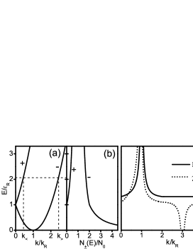
Figure 1: (a): Rashba SO split electron dispersions $\frac{\hbar^{2}}{2m}(k\pm k_{R})^{2}$ in units of $\epsilon_{R}=\frac{m}{8}\gamma_{R}^{2}$. The horizontal dashed line indicates the Fermi level. (b): density of states for the $\pm$ bands. (c): plots of $\Gamma_{k}$, Eq.(13), and $\chi_{k}$, Eq.(14).

Let us now turn to evaluate the explicit time dependence of $S_{z}$. From Eq.(10), a general solution for $S^{e}_{zk}(t)$ is given by a linear combination of $\exp\!\left(-\frac{\Gamma_{k}\pm\sqrt{\Sigma_{k}}}{2\tau_{\rm p}}t\right)$, where $\Sigma_{k}=\Gamma_{k}^{2}-\chi_{k}-(2\tau_{\rm p}\gamma_{R}k)^{2}$, whose coefficients are fixed by imposing some initial conditions. If at $t=0$ electrons have been prepared with a non-equilibrium spin-state occupation but equilibrium distribution for each spin branch then, at the lowest order in the initial weak spin imbalance $\delta\mu=(\mu_{\uparrow}-\mu_{\downarrow})/2$, $S^{e}_{zk}(0)$ is simply:

$$S^{e}_{zk}(0)=-\frac{\delta\mu}{\gamma_{R}k}\sum_{\alpha}\alpha f_{0}(E_{k\alpha}-\mu),$$ (15)

where $f_{0}(x)=(\exp(x/T)+1)^{-1}$ is the Fermi distribution function, $T$ is the temperature and $\mu\geq 0$ is the chemical potential. Furthermore, by imposing that $\lim_{t\rightarrow\infty}|S_{zk}(t)|<\infty$ and by arbitrarily choosing $dS_{z}(0)/dt=0$ for $\tau_{\rm p}^{-1}=0$, at zero temperature ($\mu=\epsilon_{F}$) $S_{z}(t)$ is readily found to be:

$$S_{z}(t) \!\!\!=\!\!\!\!\! -\frac{\delta\mu}{2\pi\gamma_{R}}\int_{k_{<}}^{k_{>}}\!dk\!\left[\theta(\Sigma_{k}-\Gamma_{k}^{2})\exp\!\left(-\frac{\Gamma_{k}+\sqrt{\Sigma_{k}}}{2\tau_{\rm p}}t\right)\right.$$ (16)

$$\left.+\theta(\Gamma_{k}^{2}-\Sigma_{k})\exp\!\left(-\frac{\Gamma_{k}}{2\tau_{\rm p}}t\right)\cosh\!\left(\frac{\sqrt{\Sigma_{k}}}{2\tau_{\rm p}}t\right)\right],$$

where $\theta$ is the unit step function, $k_{\gtrless}=k_{R}(\sqrt{\epsilon_{F}/\epsilon_{R}}\pm 1)$ for $\epsilon_{F}/\epsilon_{R}>1$ and $k_{\gtrless}=k_{R}(1\pm\sqrt{\epsilon_{F}/\epsilon_{R}})$ for $\epsilon_{F}/\epsilon_{R}<1$ [see Fig.1(a)]. For $\epsilon_{F}/\epsilon_{R}\rightarrow\infty$, $k_{\gtrless}\rightarrow k_{F}$ and Eq.(16) reduces to the classical formula

$$S_{z}(t)=S_{z}(0)\exp\!\!\left(-\frac{t}{2\tau_{p}}\right)\cosh\!\!\left(\frac{t\sqrt{1-(2\tau_{p}\Omega_{R})^{2}}}{2\tau_{p}}\right),$$ (17)

where $S_{z}(0)=-\hbar\delta\mu N_{0}$ and $\Omega_{R}=\gamma_{R}k_{F}$ is the Rashba frequency which characterizes the (damped) spin precession behavior $S_{z}(t)\approx S_{z}(0)\exp(-\frac{t}{2\tau_{\rm p}})\cos(\Omega_{R}t)$ for $2\tau_{p}\Omega_{R}\gg 1$ and the DP relaxational decay $S_{z}(t)\approx S_{z}(0)\exp(-\tau_{\rm p}\Omega_{R}^{2}t)$ for $2\tau_{p}\Omega_{R}\ll 1$ fabian .

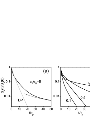
Figure 2: (a): Spin polarization time evolution from Eq.(16) (solid line) for $\tau_{p}=3.3$ fs, $\epsilon_{R}=5$ meV and $\epsilon_{F}=25$ meV. The dotted line is the power law decay of Eq.(20) while the grey solid line is Eq.(17). (b): Crossover from the power law decay of (20) and the fast relaxation decay of (21) obtained for $\tau_{p}=3.3$ fs, $\epsilon_{F}=5$ meV and several values of $\epsilon_{R}$.

For finite values of $\epsilon_{F}/\epsilon_{R}$, Eq.(16) starts to deviate from the classical regime (17). Let us first consider $\epsilon_{F}/\epsilon_{R}\geq 25$. In this case, the integration over $k$ in Eq.(16) spans values necessarily larger than $4k_{R}$, where, according to Eqs.(13,14), $\Gamma_{k}=1$ and $\chi_{k}=0$ [see also Fig.1(c)]. For weak impurity scattering ($2\tau_{\rm p}\gamma_{R}k_{<}\gg 1$) $\Sigma_{k}$ is negative and Eq.(16) reduces to:

$$S_{z}(t)\approx S_{z}(0)\exp\left(\!-\frac{t}{2\tau_{\rm p}}\!\right)\frac{\sin(\Omega_{>}t)-\sin(\Omega_{<}t)}{(\Omega_{>}-\Omega_{<})t},$$ (18)

where $\Omega_{\gtrless}=\gamma_{R}k_{\gtrless}$. The main feature of Eq.(18) is that $S_{z}(t)$ oscillates with two different Rashba frequencies $\Omega_{\gtrless}$ associated with the two SO splitted Fermi surfaces, Fig.1(a). Two distinct Rashba frequencies characterize also the relaxation regime obtained when the scattering with impurities is strong enough that $2\tau_{\rm p}\gamma_{R}k_{>}\ll 1$ (and so $\Sigma_{k}>0$) holds true. Also in this case the integration of Eq.(16) is elementary and

$$S_{z}(t)\!\approx\!S_{z}(0)\frac{\sqrt{\pi}}{2}\frac{{\rm erf}\!\left(\!\sqrt{\tau_{\rm p}\Omega_{>}^{2}t}\right)-{\rm erf}\!\left(\!\sqrt{\tau_{\rm p}\Omega_{<}^{2}t}\right)}{\sqrt{\tau_{\rm p}(\Omega_{>}-\Omega_{<})^{2}t}},$$ (19)

where ${\rm erf}$ is the error function.

The spin precession and relaxation regimes of Eqs.(18,19) are governed solely by the enhanced momentum phase space settled by finite values of $\epsilon_{F}/\epsilon_{R}$. Instead, for $\epsilon_{F}/\epsilon_{R}<25$, also the momentum dependence of $\Gamma_{k}$ and $\chi_{k}$ becomes relevant, leading to important anomalous features of the spin dynamics. One of these is particularly striking and it is found when $1\leq\epsilon_{F}/\epsilon_{R}\leq 9$. In this case, the integration over $k$ in Eq.(16) crosses the point $k=2k_{R}$ where $\chi_{k}$ changes sign [see Fig.1(c)]. Hence, if $4\tau_{\rm p}\gamma_{R}k_{R}\ll 1$, $\sqrt{\Sigma_{k}}$ can be expanded as $\Gamma_{k}-(2k_{R}-k)/3k_{R}$ for $k<2k_{R}$, while when $k>2k_{R}$ $\chi_{k}$ becomes negative leading to exponentially small contributions to $S_{z}(t)$ for sufficiently long times. Eq.(16) then can be approximated to:

$$S_{z}(t)\approx-\frac{\delta\mu}{2\pi\gamma_{R}}\int_{k_{<}}^{2k_{R}}\!\frac{dk}{2}\,e^{-\frac{(2k_{R}-k)}{6\tau_{\rm p}k_{R}}t}\approx\frac{3S_{z}(0)}{2}\frac{\tau_{\rm p}}{t}.$$ (20)

The surprising result of Eq.(20) provides the rather interesting prediction that, for sufficiently strong SO interaction and momentum scattering, the spin polarization decays as a power law rather than exponentially. In this case therefore the memory of the initial spin polarization can be much longer lived than in the DP regime, as shown in Fig. 2(a). Another striking feature is that obtained in the extreme $\epsilon_{F}/\epsilon_{R}\ll 1$ limit in which the integration of Eq.(16) becomes restricted to a narrow region around $k=k_{R}$ where both $\Gamma_{k}$ and $\chi_{k}$ diverge as $1/|k-k_{R}|$, so that Eq.(16) becomes:

$$S_{z}(t)\propto\exp\!\left(-\frac{t}{8\tau_{\rm p}}\right),$$ (21)

indicating that for extremely strong SO interaction, momentum scattering increases the spin polarization decay. The power decay of (20) and the fast relaxation regime of (21) are plotted in Fig.2(b) from a numerical integration of Eq.(16) for $\tau_{p}=3.3$ fs, $\epsilon_{F}=5$ meV and $\epsilon_{R}$ ranging from $50$ meV down to $1$ meV.

To conclude, the kinetic equations describing the time evolution of the spin polarization have been formulated for arbitrary strength of the SO interaction. Explicit solutions for quantum wells with Rashba-like SO interactions predict the failure of the DP relaxation formula for sufficiently strong SO couplings. In particular, the memory of the initial spin state can be strongly enhanced or reduced depending on $\epsilon_{F}/\epsilon_{R}$, suggesting an alternative route for spin manipulation in spintronic applications.

I thank E. Cappelluti for fruitful discussions.

References

• (1) G. Prinz, Phys. Today 48 (4), 58 (1995).
• (2) I. Ε½utiΔ‡, J. Fabian, and S. Das Sarma, Rev. Mod. Phys. 76, 323 (2004).
• (3) S. Datta and B. Das, Appl. Phys. Lett. 56, 665 (1990).
• (4) J. Schliemann, J. C. Egues, and D. Loss, Phys. Rev. Lett. 90, 146801 (2003).
• (5) E. I. Rashba, Sov. Phys. Solid State 2, 1224 (1960).
• (6) G. Dresselhaus, Phys. Rev. 100, 580 (1955).
• (7) M. I. Dyakonov and V. I. Perel, Fiz. Tverd. Tela 13, 3581 (1971) [Sov. Phys. Solid State 13, 3023 (1971)].
• (8) J. Sinova et al., Phys. Rev. Lett. 92, 126603 (2004).
• (9) Y. S. Gui et al., Phys. Rev. B 70, 115328 (2004).
• (10) E. Rotenberg, J. W. Chung, and S. D. Kevan, Phys. Rev. Lett. 82, 4066 (1999).
• (11) Yu. M. Koroteev et al., Phys. Rev. Lett. 93 046403 (2004).
• (12) E. Bauer et al., Phys. Rev. Lett. 92, 027003 (2004).
• (13) K. V. Samokhin, E. S. Zijlstra, and S. K. Bose, Phys. Rev. B 69, 094514 (2004).
• (14) M. W. Wu, J. Phys. Soc. Japan 70, 2195 (2001).
• (15) M. M. Glazov and E. L. Ivchenko, J. Supercond. 16, 735 (2003).
• (16) F. X. Bronold, A. Saxena, and D. L. Smith, Phys. Rev. B 70, 245210 (2004).
• (17) E. L. Ivchenko, Yu. B. Lyanda-Geller, and G. E. Pikus, Zh. Eksp. Teor. Fiz. 98, 989 (1990) [Sov. Phys. JETP 71, 550 (1990)].
• (18) A. A. Burkov, A. S. NΓΊΓ±ez, and A. H. MacDonald, Phys. Rev. B 70, 155308 (2004).
• (19) C. Lechner and U. RΓΆssler, cond-mat/0412370 (2004).
• (20) K. Blum, Density Matrix Theory and Applications (Plenum, New York, 1981).
• (21) T. Kuhn and F. Rossi, Phys. Rev. B 46, 7496 (1992).
• (22) The following results are equally valid for quantum wells with zero Rashba interaction but with a Dresselhaus coupling of the form $\mathbf{\Omega}_{\bf k}=(\gamma_{D}k_{x},-\gamma_{D}k_{y},0)$.