The mean field infinite range $p=3$ spin glass: equilibrium landscape and correlation time scales

Abstract

We investigate numerically the dynamical behavior of the mean field 3-spin spin glass model: we study equilibrium dynamics, and compute equilibrium time scales as a function of the system size $V$. We find that for increasing volumes the time scales $\tau$ increase like $\ln\tau\propto V$. We also present an accurate study of the equilibrium static properties of the system.

I Introduction

The glassy state is a state of matter ubiquitous in nature. It enjoys a number of intriguing properties: among those is the amazingly slow dynamics, common to both structural glasses and spin glasses. It is surely not well understood, and during the last years it has been the subject of numerous investigations, both theoretical and experimental.

One interesting approach, first used for studying spin glasses in MACYOU , is based on (optimized) Monte Carlo numerical simulations. One considers samples that can be brought to equilibrium (in order to do that the lattice size cannot be too large) and studies numerically the equilibrium dynamics of the system (this is typically not what happens with real disordered systems of this type, that are forever out of equilibrium).

The method was first used to investigate the dynamics of the mean field Sherrington–Kirkpatrick (SK) model MACYOU ; BIMA : it turns out BIMA that all the relevant time scales $\tau_{\alpha}$ of the model grow for diverging lattice sizes $V$ according to the scaling law $\ln\left(\tau_{\alpha}\right)\propto V^{1/3}$. A single time scale controls the critical behavior of the model: the time scale governing the mode leading from $\cal A$, one of the many equilibrium states of the mean field theory, to a different state $\cal B$ (not related to $\cal A$ by a global spin flip) has the same scaling law that the time scale controlling the mode related to a $Z_{2}$ global inversion (leading from a state to its $Z_{2}$ symmetric).

We will deal here with the case of the mean field, fully connected $p$-spin spin glass, with $p=3$, and try to determine the relevant time scales. Recently Ioffe, Lopatin and Sherrington have developed IOIOSH a theoretical analysis of the problem: their approach suggests that for this class of models the relevant time scale behaves as $\ln\left(\tau_{\alpha}\right)\propto V$ (see also the work of BIBRKO for a computation of relaxation times in spin systems with disordered quenched couplings). Here we try to analyze the model to uncover the true asymptotic behavior by using the numerical approach of MACYOU ; BIMA .

The fully connected $p$-spin model is a generalization of the SK mean field spin glass to a model where interaction is given by products of $p$ spins (the $p=2$ model coincides with SK): it turns out to be a promising candidate to understand the physics of structural glasses MEPAVI ; KI . Numerical simulations of this model are extremely CPU time and memory consuming: one needs to store order of $V^{p}$ quenched random couplings, and the time needed to run a Metropolis sweep increases with volume like $V^{p}$, as compared to $V$ for short range models. Furthermore, glassy slow dynamics has to be studied for very large times. Here why study the $p=3$ fully connected model: it is already quite expensive, but the cheapest of its class (we do not loose in generality since all models with $p\geq 3$ are believed to have the same universal behavior).

In the next section we give details about our numerical simulations. We use parallel tempering PARTEM , an optimized Monte Carlo method very effective on spin glass systems . As an added bonus we present in the following section very precise results about the statics of the system: these are by far the most accurate results obtained for equilibrium expectations in this model (see PIRISA for the former state of the art). They allow to compare the $N=\infty$ analytic results with finite $N$ accurate values, and to get a feeling about what a “large” lattice really is. They also help in making us confident that we are really reaching thermodynamic equilibrium. The evidence collected here is interesting since, although this model is very important for reaching an understanding of the glassy phase, it has never been studied numerically with high accuracy, because of the extreme difficulty of the simulation.

In a fourth section, we present our main results, about time scales in the model. We find that the Ioffe–Lopatin–Sherrington approach leads indeed to the correct estimate, and that $\ln\left(\tau_{\alpha}\right)\propto V$. We end by drawing our conclusions.

II Numerical Simulations

The infinite range, fully connected, $3$-spin spin glass is defined by the Hamiltonian

$${\cal H}\equiv-{\displaystyle\sum_{i<j<k}J_{i,j,k}\ \sigma_{i}\,\sigma_{j}\,\sigma_{k}}\ ,$$ (1)

where the quenched random exchange coupling $J_{i,j,k}$ govern the interaction among triples of spins and can take one of the two values $\pm\sqrt{3}/V$ with probability one half. The choice we made of binary couplings allows far superior performances of the computer code.

The model has a complex phase diagramGARDNER ; CAPARA ; MORITE . From a thermodynamic point of view it has three phases. At high $T$ it is in a paramagnetic replica symmetric (RS) phase. At $T=T_{c}$ the system enters a one-step replica symmetry breaking (1RSB) phase, while at a lower temperature value $T_{G}<T<T_{c}$ it enters a third phase that will not concern us here.

The order parameter is the usual overlap $q$. Its probability distribution function can be written as

$$P(q)\equiv\frac{1}{V}\overline{\left\langle\delta(q-\sum_{i}\sigma_{i}\tau_{j})\right\rangle}\ ,$$ (2)

where, as usual, the brackets denote a thermal average and the over-line denotes an average over the quenched random couplings. In the RS phase, in the infinite volume limit, two different replica have zero overlap. In the 1RSB phase two different replica have overlap $q_{0}=0$ with probability $m$, and overlap $q_{1}>0$ with probability $1-m$ (both $q_{1}$ and $m$ depend on temperature, and should be written $q_{1}(T)$ and $m(T)$). The values of $m$ and $q_{1}$ are solutions of a set of two coupled integral equations. The condition $m=1$ gives the value of the critical temperature $T_{c}\approx 0.6514$ (the expansion around the large $p$ limit of GARDNER gives $T_{c}\approx 0.6671$, and $T_{G}\ \approx 0.24$). It turns out that $\lim_{T\to T_{c}^{-}}q_{1}(T)\neq 0$, namely the model has discontinuous 1RSB.

\psfrag{x}[c][c][0.75]{$T$}\psfrag{y}[r][r][0.75][-90]{$E(T)$}\includegraphics[width=143.09538pt,angle={270}]{en_color.eps}

Figure 1: The internal energy as a function of the temperature. The continuous curve is from the analytical solution of the model. Numerical data are for system sizes from $32$ to $192$.

\psfrag{x}[c][c][0.75]{$T$}\psfrag{y}[r][r][0.75][-90]{$E(T)$}\includegraphics[width=143.09538pt,angle={270}]{c_color.eps}

Figure 2: As in figure 1, but for the specific heat.

Let us start by giving some details about our simulation. We study systems with $V=32$, $64$, $96$, $128$, $160$ and $192$ spins (the needed CPU time increases with volume like $V^{3}$). We first thermalize the system using the parallel tempering optimized Monte Carlo procedure PARTEM , with a set of $15$ $T$ values in the range $0.3-1.2$ (i.e. $\Delta T=0.06$) for the three smallest volumes and with $\Delta T=0.03$ in the temperature range $0.3-0.9$ for the three largest volumes. We take advantage of the binary distribution of the couplings to use the multi-spin coding techniqueMSC , with a one order of magnitude gain in update speed. We perform $4\cdot 10^{5}$ iterations (one iteration consists of one Metropolis sweep of all spins plus one tempering update cycle), and store the final well equilibrated configurations.

\psfrag{x}[c][c][0.75]{$T$}\psfrag{y}[r][r][0.75][-90]{$\bar{q}(T)$}\includegraphics[width=143.09538pt,angle={270}]{q_color.eps}

Figure 3: The order parameter $\bar{q}$ as a function of the temperature. The continuous curve is from the analytical solution of the model. Data are for system sizes from $32$ to $192$.

We then, for studying the dynamical behavior of the system, start updating these equilibrium configurations with a simple Metropolis dynamics, and perform $2\cdot 10^{6}$ Metropolis sweeps. The number of disorder samples is $1000$ for the $V=32$ system, $500$ for $V=64$ and $200$ for the other, larger, sizes. As usual, the program simulates the independent evolution of two replicas, in order to compute the overlap $q$. All statistical error estimates are done using a jackknife analysis of the fluctuations among disorder samples, with $20$ jackknife bins.

We have used the second half of the $4\cdot 10^{5}$ thermal sweeps, i.e. the last $2\cdot 10^{5}$, to measure static quantities. This is on the one side an interesting result on his own (since we can compare to the analytic, $N=\infty$, result, and get hints about how finite $N$ corrections work), and allows, on the other side, to check thermalization. Notice that our largest thermalized system is more than five times larger than the largest analyzed before PIRISA : we will present next these results, before discussing the dynamical behavior of the system.

III Static Behavior

\psfrag{x}[c][c][0.75]{$q$}\psfrag{y}[r][r][0.75][-90]{$P(q)$}\includegraphics[width=143.09538pt,angle={270}]{pq_color.eps}

Figure 4: Probability distribution function of the overlap, for system sizes from $32$ to $192$. Here $T=0.42$.

\psfrag{x}[c][c][0.75]{$T$}\psfrag{y}[r][r][0.75][-90]{$B(T)$}\includegraphics[width=143.09538pt,angle={270}]{b_color.eps}

Figure 5: Binder parameter as a function of the temperature. The continuous curve is from the analytical solution of the model.

We show in figure 1 our data for the internal energy $E={\overline{\left\langle{\cal H}\right\rangle}}/{V}$ as a function of the temperature (we average this single replica quantity over the two copies of the system that we follow in parallel), together with the analytical result

$$E=-\frac{1}{2T}\left(1-\left(1-m\right)q_{1}^{3}\right)\ .$$ (3)

The finite volume numerical data converge nicely toward the infinite volume limit analytical curve. This statement can be make quantitative by fitting to some assumed analytical finite size behavior. Taking $T=0.3$ as an example, a good representation of the data is obtained with the simple form $E_{V}=E_{\infty}+aV^{-1/\vartheta}$: by using for $E_{\infty}$ the exact analytic value, one finds that a best fit gives $\vartheta=1.13\pm 0.01$. In figure 2 we show the specific heat: again, the approach to the infinite volume result is very clear in the numerical data.

\psfrag{x}[c][c][0.75]{$T$}\psfrag{y}[r][r][0.75][-90]{$A(T)$}\includegraphics[width=143.09538pt,angle={270}]{a_color.eps}

Figure 6: The $A$ parameter as a function of the temperature. The continuous curve is from the analytical solution of the model.

We show in figure 3 the order parameter $\overline{q}=\overline{\left\langle q\right\rangle}$, together with the theoretical result $(1-m)q_{1}$, as a function of the temperature: we find again an excellent convergence to the infinite volume limit.

We show in figure 4 the overlap probability distribution (for $T=0.42$). Data are in agreement with the prediction of a bimodal probability distribution, that becomes sharper and sharper as $V$ grows: one peak is around zero and the other around some positive value of $q$. Between the two peaks the probability distribution vanishes in the large volume limit, as predicted by the 1RSB picture (and in contrast to $\infty$RSB).

Figures 5 and 6 are for the usual Binder parameter

$$B\equiv\frac{1}{2}\Bigl{(}3-\frac{\overline{\left\langle q^{4}\right\rangle}}{\overline{\left\langle q^{2}\right\rangle}^{2}}\Bigr{)}\ ,$$ (4)

and for the $A$ parameter that measures order-parameter fluctuations

$$A=\frac{\overline{\left\langle q^{2}\right\rangle^{2}}-\overline{\left\langle q^{2}\right\rangle}^{2}}{\overline{\left\langle q^{2}\right\rangle}^{2}}\ .$$ (5)

As shown in reference PIRISA , $B$ and $A$ have very simple expression as a function of $m$, since for $q_{0}=0$ there is no residual dependence on $q_{1}$ and one gets that both $B$ and $A$ are equal to zero in the high $T$ phase, and that:

$$B = \frac{2-3m}{2(1-m)}\qquad T_{G}<T<T_{c}\ ,$$ (6)

$$A = \frac{m}{3(1-m)}\qquad T_{G}<T<T_{c}\ .$$ (7)

Note that we are in a non-standard case where some dimensionless quantities diverge at $T_{c}$: in this model both $B$ and $A$ diverge as $T\to T_{c}^{-}$. This is in marked contrast with usual cases, where both $B$ and $A$ have a finite limit for all temperatures as $V\to\infty$.

Our numerical data are consistent with the predictions: namely they show a zero limit in the RS phase, and a nonzero limiting curve, that diverges as $T\to T_{c}$, in the 1RSB phase (data are consistent with both the maximum of $A$ and the minimum of $B$ being proportional to $V$). In other words, in this situation one finds, neither for $B$ nor for $A$, a fixed point where the curves for increasing values of $V$ cross. Absence of crossing for the Binder parameter has been also observed in HUKUKAWA for the infinite range $3$ state Potts spin glass model (a model with continuous 1RSB) and in BIBRKO for the $10$ state model (a model with discontinuous 1RSB). The fact that $A$ has a non-trivial limit as $V$ grows shows clearly that the model has non-zero order parameter fluctuations (OPF) in the 1RSB phase, and the effectiveness of the parameter $A$ to determine whether OPF holds or not.

IV Dynamical Behavior

\psfrag{x}[c][c][0.75]{$t$}\psfrag{y}[r][r][0.75][-90]{$q^{c}(0,t)$}\includegraphics[width=143.09538pt,angle={270}]{q1c_color_ok.eps}

Figure 7: $q^{c}(0,t)$ as a function of $t$ (in log scale) in units of Metropolis sweeps. Here $T=0.48$.

The main result of this note is the precise quantitative measurement of the typical time scales of the model and of their scaling behavior. As we have already discussed we use the approach of MACYOU ; BIMA , considering the equilibrium dynamics of thermalized configurations.

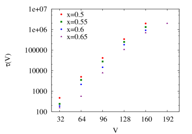
Figure 8: $\tau_{X}$ (in log scale) as a function of the number of spins $V$, for $X=0.5$, $0.55$, $0.6$ and $0.65$. $T=0.48$.

We measure the time dependent overlap of two spin configurations:

$$q(0,t)\equiv\left\langle\frac{1}{N}\sum_{i}\sigma_{i}(0)\sigma_{i}(t)\right\rangle\ ,$$ (8)

where we start, at time zero, from an equilibrium spin configuration (see the former two sections), and the time $t$ is measured in units of Metropolis sweeps (in this phase of the numerical simulation we are using the simple Metropolis dynamics: we use parallel tempering only in the first phase of thermalization and equilibrium analysis). The thermodynamic average $\left\langle\dots\right\rangle$ is taken by averaging over several initial configurations. As noticed in MACYOU , the best and most effective way to proceed is to use a new disorder sample for every simulation: we do never repeat simulations with different starting points in a given disorder sample, but always use new quenched random couplings when starting a new numerical run. This procedure correctly averages over the thermal noise and over the random couplings, by minimizing the statistical incertitude (mainly connected to the sample average): no bias is introduced. In what follows, the average $\left\langle\dots\right\rangle$ is accordingly an average over two independent replicas only.

As $t$ goes to infinity, $q(0,t)$ coincides with the static overlap, and it is distributed according to the probability distribution $P(q)$. Accordingly (on a finite system)

$$q^{c}(0,t)\equiv\overline{q(0,t)}-\bar{q}\to 0\qquad as\ t\to\infty.$$ (9)

Our results for $q^{c}(0,t)$ as function of the Metropolis time (note the logarithmic scale) for $T=0.48$ can be found in figure 7 ($T_{c}\approx 0.6514$, so we are at $T\sim\frac{2}{3}T_{c}$). The behavior of $q^{c}(0,t)$ is very clear. On the largest lattices we are able to study, the time evolution has two successive regimes as $t$ grows: first $q^{c}(0,t)$ decays very slowly toward the value $q_{1}$ (the equivalent of $q_{EA}$ in spin glass models). It stays in this first regime longer and longer as the system size increases (and would stay there forever in the infinite system size limit). In a second regime, $q^{c}(0,t)$ goes to zero, and the system equilibrates.

\psfrag{x}[c][c][0.75]{$V$}\psfrag{y}[r][r][0.75][-90]{$\tau_{1/2}$}\includegraphics[width=143.09538pt,angle={270}]{tau_bw.eps}

Figure 9: $\tau_{1/2}$ (in log scale) as a function of the number of spins $V$. $T=0.54$.

We need now to define a typical time scale of the equilibrium dynamics. We use the simple approach based on selecting a time such that the (normalized) correlation decreases below a given threshold $X$. We tried several values of this threshold to check the stability of this definition. So our time scale $\tau_{X}$ is defined as the time such that $q^{c}(0,t=\tau_{X})=X\ q^{c}(0,0)$. Technically if the numerical data cross the level $X$ more than once we average over all crossing point (this is not a big issue, since we never find a real ambiguity, but only sometimes a small wiggling, due to statistical fluctuations, very local in time). We now examine the values of $\ln\tau_{X}$ as a function of $V$. If there is only one diverging time scale in the problem, the behavior of $\tau_{X}$ as function of $V$ should not depend on $X$. We show the data obtained by this analysis in figure 8 (for $T=0.48$): there is indeed a remarkable level of universality, and the scaling law of the data is clearly independent of $X$, making us confident about the quality of our approach. Notice that we are changing the threshold $X$ in a large range of values, and the results are stable: this is a very good indication toward the fact that we are really determining the physical time scales.

In figure 9 we show our data for $\tau_{1/2}$ at $T=0.54$, together with the best fit of the data to the expression

$$\tau\left(V\right)=A\ e^{BV^{\epsilon}}\ ,$$ (10)

with the values $A=35\pm 10$, $B=\left(4.5\pm 2.0\right)\cdot 10^{-2}$ $\epsilon=1.0\pm 0.1$, with a value of chi-square $\chi^{2}=1.8$ per degree of freedom.

These numerical results are in remarkable agreement with the predictions of IOIOSH : in the broken symmetry phase the typical and relevant time scales grow here according to $\ln(\tau)\propto V$, as opposed to the Sherrington–Kirkpatrick, $p=2$ model, where they grow according to $\ln(\tau)\propto V^{\frac{1}{3}}$ BIMA . Here the absence of visible sub-leading corrections is remarkable, in contrast again to the situation of the Sherrington–Kirkpatrick model where the small exponent $1/3$ makes things difficult.

V Conclusions

We have studied the $3$-spin infinite range spin glass model. We have determined with good accuracy equilibrium properties on lattices of reasonable size, gaining in this way an accurate control of finite size effects. The main point of this note has been to investigate the equilibrium dynamics of the model, and to establish that the time scales of the model grow with system size $V$ according to the law $\ln\tau_{\alpha}\propto V$: this is in nice agreement with the prediction of the theoretical approach by IOIOSH . Technically, from the computational point of view, these results are worthy because simulating a $3$-spin infinite range model is a very non-trivial task: here the computer time needed to perform a full update of the lattice increases as $V^{3}$ for large volumes. We have succeeded on the one side to study the statics of the model on lattice more than five times bigger than the largest ones used before, and on the other side to determine with good accuracy severely increasing time scales: we consider that as a worthy achievement.

VI Acknowledgments

We acknowledge enlightening discussions with David Sherrington in Les Houches and on Montagne Sainte-Geneviève. We are especially grateful to Giorgio Parisi for pointing out to us a series of typographical misadventures that plagued a first version of the text. The numerical simulations have been run on the PC cluster Gallega at Saclay.

References

- (1) N. D. Mackenzie and A. P. Young, Phys. Rev. Lett. 49, 301 (1982); N. D. Mackenzie and A. P. Young, J. Phys. C 16, 5321 (1983).
- (2) A. Billoire and E. Marinari, J. Phys. A 34, L727 (2001).
- (3) L. B Ioffe and D. Sherrington, Phys. Rev. B 57, 7666 (1998); A. V. Lopatin and L.B. Ioffe, Phys. Rev. Lett. 84, 4208 (2000); A. V. Lopatin and L.B. Ioffe, Phys. Rev. B 60, 6412 (1999).
- (4) C. Brangian, W. Kob, and K. Binder, Europhys. Lett. 53, 756 (2001); J. Phys. A: Math. Gen. 35, 191 (2002).
- (5) M. Mézard, G. Parisi and M. A. Virasoro, Spin Glass Theory and Beyond (World Scientific, Singapore 1987).
- (6) T. R. Kirkpatrick and D. Thirumalai, Phys. Rev. B 36, 5388 (1987).
- (7) K. Hukushima and K. Nemoto, J. Phys. Soc. Japan 65, 1604 (1996); M. C. Tesi, E. J. Janse van Rensburg, E. Orlandini and S. G. Whittington, J. Stat. Phys. 82, 155 (1996); E. Marinari, Optimized Monte Carlo Methods in Advances in Computer Simulation, edited by J. Kertesz and I. Kondor, Springer-Verlag (1997).
- (8) M. Picco, F. Ritort and M. Sales, Eur. Phys. J. B 19, 565 (2001).
- (9) D. Gross and M. Mézard, Nucl. Phys. B240, 431 (1984); E. Gardner, Nucl. Phys. B 257, 747 (1985).
- (10) M. Campellone, G. Parisi and P. Ranieri, Phys. Rev. B 59 1036 (1999).
- (11) A. Montanari and F. Ricci-Tersenghi, Eur. Phys. J. B 33 339 (2003).
- (12) H. Rieger, HLRZ 53/92, hep-lat/9208019; our code is based on F. Zuliani (1998), unpublished.
- (13) K. Hukushima and H. Kawamura, Phys. Rev. E 62 3360 (2000).