Effect of electronic interactions on the persistent current in one-dimensional disordered rings

Abstract

The persistent current is here studied in one-dimensional disordered rings that contain interacting electrons. We used the density matrix renormalization group algorithms in order to compute the stiffness, a measure that gives the magnitude of the persistent currents as a function of the boundary conditions for different sets of both interaction and disorder characteristics. In contrast to its non-interacting value, an increase in the stiffness parameter was observed for systems at and off half-filling for weak interactions and non-zero disorders. Within the strong interaction limit, the decrease in stiffness depends on the filling and an analytical approach is developed to recover the observed behaviors. This is required in order to understand its mechanisms. Finally, the study of the localization length confirms the enhancement of the persistent current for moderate interactions when disorders are present at half-filling. Our results reveal two different regimes, one for weak and one for strong interactions at and off half-filling.

I Introduction

Mesoscopic rings are known to carry an equilibrium current called persistent currents when they are threaded through a magnetic flux buttiker83 . The experimental discovery levy90 ; chandra91 ; mailly93 of persistent currents has motivated a number of theoretical studies. For example, non-interacting electron theories oppen91 ; altshuler91 ; schmid91 describe the general features but they strongly underestimate the current present within the diffusive regime jariwala01 . The fact of taking into account either electron-electron interactions loss92 or simply the degree of disorder montambaux90 leads to an underestimation and hence, only a partial description of the magnitude of the currents. A possible way to improve the characterization of the persistent currents is to take into account both disorder and electronic interactions pctheory . Unfortunately, this has proved to be a difficult problem to tackle. Diagrammatic perturbative expansion in three dimension suggests an increase in the current ambegoakar90 but does not provide the means to conclude firmly. Therefore, we restricted the problem here to one dimension. Surprisingly, the role of electronic interactions is still a controversial question and some have even suggested that such interactions may lead to a decrease in the magnitude of the persistent currents georges94 ; kato94 . On the one hand, experiments using exact diagonalization for systems containing very few lattice sites berkovitz93 and the self-consistent Hartree-Fock approximation kato94 ; Cohen98 show that repulsive interactions suppress the persistent currents whereas calculations show no dramatic increase in the magnitude of the persistent currents berkovitz93 ; abraham93 . On the other hand, DMRG numerical studies carried out on spinless fermions claim to obtain a small increase in the magnitude of the persistent currents for very high disorder only schmitteckert98 . It has also been shown that repulsive interactions may provoke significant disorder and hence, enhance the electron mobility shepelyansky94 ; benenti99 in few-particle models. The need to take into account the spin has also theoretically been investigated using the method of bosonization thierry95 . The result suggests that the stiffness could be enhanced by intermediate interactions. Numerical approaches roemer95 ; mori96 further show that repulsive interactions enhance the persistent currents in weakly disordered systems off half-filling only.

In this paper, we consider a simplified model of interacting electrons in a one-dimensional disordered ring, which is penetrated by a magnetic flux. It has been reported in another study that moderate interactions could induce an enhancement of the persistent currents even in the presence of weak disorder for half-filled systems gambetti02 . Moreover disorder could have the unexpected effect of increasing the zero-temperature persistent currents in one-dimensional half-filled Hubbard rings, with strongly interacting electrons. We emphasize that even off half-filling the persistent current may still be enhanced by small interactions and in such case, the filling may have an influence on its behavior. Indeed, we show that the behavior of the persistent currents changes as it is moved off half-filling, owing to the appearance of holes. These results are established partially within the framework of the strong coupling perturbation expansion and partially through numerical calculations by means of the Density Matrix Renormalization Group algorithm DMRGbasics ; white92 . Finally, we study the influence of the spin on the behavior of the stiffness parameter and show that the case of half-filling is rather particular. This manuscript gambettithese04 is organized as follows. In Section II, the model and the calculation algorithms of the persistent currents are presented. The numerical and analytical work at half-filling are presented in section III. Section IV contains the numerical results off half-filling and further explains the results by means of the perturbation expansion. Section V highlights the influence of the spin not only on the stiffness parameter, but also on the magnitude of the persistent currents. Section VI is devoted to the study of the localization length and identifies two regimes that are characterized by weak and strong interactions, which are separated by a crossover phase. Finally, our conclusions are presented in section VII. Details of the analytical approaches used in Sections III and IV are given in Appendices A.1 and A.2. A toy model is developed for non half-filled systems in Appendix A.3. Appendix B concerns the behavior of the weights of the ground-state in the strong interaction limit. In Appendix C, the specific case of an odd number of electrons present in a ring is discussed.

II Model and Method

A one-dimensional lattice is shown in function of the Hubbard-Anderson Hamiltonian Hubbard57Anderson59 , which we use to describe N interacting electrons in a disordered ring of M sites:

$$H=H_{K}+H_{W}+H_{U}$$ (1)

$$H_{K}=-t\sum_{i=1}^{M}\sum_{\sigma=\uparrow,\downarrow}\left(c_{i,\sigma}^{\dagger}c_{i-1,\sigma}^{\phantom{\dagger}}+c^{\dagger}_{i-1,\sigma}c_{i,\sigma}^{\phantom{\dagger}}\right)\,,$$ (2)

denotes the kinetic energy, $t$ will be set equal to one in the numerical part.

$$H_{W}=W\sum_{i=1}^{M}\sum\limits_{\sigma}v_{i}n_{i,\sigma}$$ (3)

stands for the disorder with $v_{i}\in[-\frac{1}{2},\frac{1}{2}]$, $W>0$ and finally

$$H_{U}=U\sum_{i=1}^{M}n_{i,\uparrow}n_{i,\downarrow}$$ (4)

accounts for the electronic interactions.

The threading of the ring by a magnetic flux introduces an Aharonov-Bohm phase $\Phi=2\pi\phi/\phi_{0}$ measured in units of the flux quantum $\phi_{0}=hc/e$. According to Bayers and Yang bayersyang the only effect of the magnetic field is to impose twisted boundary conditions $c_{0,\sigma}=c_{M,\sigma}\exp{i\Phi}$ between the first and the last site, the other pieces of the Hamiltonian remain unchanged. The persistent currents that are carried through an isolated ring are the direct consequence of the sensitivity of the eigenenergies to a phase-change in the boundary conditions, in particular for

$$I(\phi)=-\frac{\partial{E_{0}(\phi)}}{\partial{\phi}}\,,$$ (5)

at vanishing temperature where $E_{0}(\phi)$ denotes the ground-state energy. It has been shown that transport properties are related to thermodynamic properties in a localized system at vanishing temperature kohn64 . In fact, persistent current are a periodic function of the flux $\phi$,

$$I(\Phi)=\left(E(0)-E(\pi)\right)\sin{\Phi}\cdot\frac{\pi}{\phi_{0}}\,.$$ (6)

where

$$E(0)-E(\pi)=\Delta E$$ (7)

is called phase sensitivity. We furthermore introduce the stiffness, given by

$$D=\frac{M}{2}|\Delta E\,|,$$ (8)

which is related to the Drude weight $D_{C}$ kohn64 . We compute $D$ because it is simpler to calculate than the conductivity $\sigma$, and because it furthermore allows for a measure of the magnitude of the persistent currents. The energy levels are computed by means of the density matrix renormalization group method DMRG white92 ; DMRGbasics and exact diagonalization. The first version of the program was written by P. Brune brune for the ionic Hubbard model. Since $H$ is invariant under rotation around the $z$-axis its eigenstates can be calculated by restricting it to the subspace $S_{z}=0$. We used eight finite-lattice iterations and kept a maximum of 700 states per block iteration.

III Half-filling

The case of half-filling is here considered when the number of sites is equal to the number of electrons $M=N$.

The very strong interaction limit can be treated analytically in order to better comprehend the behavior of the phase sensitivity within the Mott insulator limit. When $U\gg W,~{}t$ the interaction $U$ dominates, and it is possible to expand $\Delta E$ in terms of $t/U$ bouchiath89 ; Dietmar01 . The details of the calculation are given in Appendix A.1. The basis-states $|\Psi_{\alpha}\rangle$ of $H_{0}$ spanning the $\alpha$-space auerbach94 are given by the product of the different on-site states, and read as follows:

$$|\psi_{\alpha}\rangle=\left(\prod_{k=1}^{N/2}c_{i^{\uparrow}_{k}(\alpha),\uparrow}^{\dagger}\right)\left(\prod_{k=1}^{N/2}c_{i^{\downarrow}_{k}(\alpha),\downarrow}^{\dagger}\right)|0\rangle\,.$$ (9)

The function $i_{k}^{\uparrow(\downarrow)}(\alpha)$ specifies the site where the $k^{\mathrm{th}}$-electron with spin $\uparrow$ ($\downarrow$) among the $N/2\uparrow(\downarrow)$-electrons is created following the configuration $\alpha$. The $|0\rangle$ state is composed of $M$ empty sites. The symbol $|\Psi_{\beta}\rangle$ denotes states that do not possess doubly-occupied sites (exactly one electron per site is present at half-filling), spanning the $\cal{S}$-space; $|\Psi_{\gamma}\rangle$ denotes states that contain at least one doubly-occupied site spanning the $\cal D$-space. The corresponding many-body energies of the states $|\psi_{\alpha}\rangle$ are summed over the disorder contributions $E_{\alpha}^{\rm W}$ and the interaction energies $E_{\alpha}^{\rm U}$. They are equal to:

$$E_{\alpha}= W\sum_{k}\left(v_{i^{\uparrow}_{k}(\alpha)}+v_{i^{\downarrow}_{k}(\alpha)}\right)+ Ug_{\alpha}\,.$$ (10)

Here $g_{\alpha}$ stands for the number of doubly-occupied sites. In the Mott insulator limit when $U\gg W,t$ the $|\Psi_{\gamma}\rangle$’s possess a very high energy level and hence, a gap arises with the $|\Psi_{\beta}\rangle$’s.

First, we consider the case without disorder. The $|\Psi_{\beta}\rangle$’s are the basis-states and all possess an equal zero energy level. Hence, for very large $U$, $H=H_{0}+H_{W}$ and the kinetic energy term $H_{K}$ represents a perturbation with respect to the dominating term $H_{U}$. Within the limit of $U\gg t$, the spin degree of freedom can be treated as a significant spin Hamiltonian that is in fact the antiferromagnetic Heisenberg Hamiltonian when $\phi=0$, for the case of the clean system lieb62 ; lieb93 ; auerbach94 . The antiferromagnetic Heisenberg Hamiltonian ground-state is the superposition of all states with a total spin equal to zero. It is furthermore non-degenerate. This theorem has been extended to the half-filled Hubbard model lieb62 ; lieb93 for an even number of sites $M$ lieb93 ; tasaki95 and the ground-state can be expressed as:

$$|\psi_{0}\rangle=\sum_{\beta}f_{\beta}\left(\prod_{k=1}^{N/2}c_{i^{\uparrow}_{k}(\beta),\uparrow}^{\dagger}\right)\left(\prod_{k=1}^{N/2}c_{i^{\downarrow}_{k}(\beta),\downarrow}^{\dagger}\right)|0\rangle$$ (11)

where the $0<f_{\beta}<1$, according to Marshall’s theorem marshall55 , for all spin configurations $\beta$ in the subspace $\cal S$ and $i_{k}^{\uparrow}\neq i_{k^{\prime}}^{\downarrow}\forall k\neq k^{\prime}$. The ground-state for $\Phi=\pi$ is equal to that presented in eq. (11).

Now we calculate the leading contributions to the phase sensitivity $\Delta E$ using the difference present in the higher-order corrections of the many-body ground-state energies under periodic and antiperiodic boundary conditions. Studying the Hubbard Hamiltonian within the strong interaction limit, is equivalent to studying the action of $H_{K}$ in the $\cal S$-space tasaki95 . Indeed, the numerator of $E^{(n)}$ is composed of matrix elements $\langle\psi_{\gamma_{l}}|H_{K}|\psi_{\gamma_{l+1}}\rangle$ of the hopping part of the Hamiltonian, which connects each site to its neighbor. Thus, the resulting correction brought to the ground-state energy $E^{(n)}$ is different from zero only when all $|\psi_{\gamma}\rangle$ states can be connected by one-particle hopping processes Dietmar01 ; selva00 . These sequences are called ${\bf A}^{(\beta,\beta^{\prime})}$ and start at $|\psi_{\beta}\rangle$ and end at $|\psi_{\beta^{\prime}}\rangle$, with the intermediate states being all $|\psi_{\gamma}\rangle$’s. In order to calculate the difference between periodic and antiperiodic boundary conditions, the particles must circle the ring and cross the border once. The lowest contributions are of order $M$, and in such case, the energy corrections for periodic and antiperiodic conditions differ only by the sign. Intermediate results are given in an already published article gambetti02 .

Second, we reintroduce disorder. The $\cal S$-states follow Mott-insulator configurations and all possess a similar and lowest energy level that reads $E_{0}^{W}=W\sum_{i=1}^{M=N}v_{i}$ (from eq. (10)). This energy level is independent of the spin configurations of the $\cal S$-states and consequently, within this limit, they degenerate and are characterized by the same weights $f_{\beta}(U\to\infty)$. All the terms in the denominator are calculated by differences between disorder and interaction contributions of the ground-state $|\Psi_{0}\rangle$ and the intermediate state $|\Psi_{\gamma_{l}}\rangle$. The denominators are written as $Wd_{\gamma_{l}}+g_{\gamma_{l}}U$. We further define $(E_{\gamma_{l}}^{\rm W}-E_{0}^{\rm W})=Wd_{\gamma_{l}}$, as the energy difference between the disorder configurations of the state $|\Psi_{0}\rangle$ and the state $|\Psi_{\gamma_{l}}\rangle$. We develop $\Delta E$ in powers of $\frac{W}{U}$ up to second order. This yields :

$$\Delta E^{(M)}\approx\frac{(-1)^{N/2}4t^{M}}{U^{M-1}}\sum_{\beta,\beta^{\prime}}\sum\limits_{{\bf A}_{\rm f}^{(\beta,\beta^{\prime})}}\frac{f_{\beta}f_{\beta^{\prime}}}{\prod_{l}g_{\gamma_{l}}}$$

$$\left(1+\frac{W^{2}}{U^{2}}\left(\sum_{l}\frac{d_{\gamma_{l}}^{2}}{g_{\gamma_{l}}^{2}}+\sum_{l<m}\frac{d_{\gamma_{l}}d_{\gamma_{m}}}{g_{\gamma_{l}}g_{\gamma_{m}}}\right)\right).$$ (12)

This sum is performed over all forward hopping sequences ${\bf A}_{\rm f}^{(\beta,\beta^{\prime})}$ (for the electrons that are moving in the anti-trigonometric direction of motion) with a first factor 2 introduced for the backward sequences and an additional factor 2 accounting for the difference between periodic and antiperiodic contributions. All contributing sequences lead to a cyclic perturbation of the $N/2$ operators corresponding to electrons with a specific spin direction. Since the weights $f_{\beta}$ are all positive, the sign of the phase sensitivity at strong interaction is given by $(-1)^{N/2}$ in eq. (III), as in the non-interacting case Leggett . The dominating term in eq. (III) (corresponding to the clean limit $W\rightarrow 0$) exhibits an interaction-induced suppression of the persistent current $\propto U(t/U)^{M}$. The first-order correction in $W/U$ totally vanishes due to the particle-hole symmetry. The second-order correction is positive because the first term is positive, and much larger than the second one. We conclude that the phase sensitivity has positive corrections for order $(\frac{W}{U})^{2}$. This conclusion is also true for the stiffness parameter, as $D=\frac{M}{2}|\Delta E|$. The unexpected conclusion is that at half-filling, the disorder increases both the phase sensitivity and the magnitude of the persistent currents for highly interacting electrons in Hubbard-Anderson rings gambetti02 . This counterintuitive effect lee85kramer93 might also be related to a competition between the phenomenon, disorder and interaction. The ground-state energy, which is equal to $E_{0}=W\sum_{i}v_{i}$ increases with the strength of the disorder W, and when $W\leq U$, the energy level becomes comparable to the interaction strength $U$. Under these conditions, the gap reduces between the energy levels of the excited states $|\Psi_{\gamma}\rangle$ and the ground-state. A jump to a doubly-occupied site is then rendered easier and thus, the movement of the electrons around the ring is favored, enhancing the magnitude of the persistent currents. These sets of $M$ hops illustrate a simple mechanism that can explain the changes in the magnitude of the persistent currents under strong interaction limits.

Extensive numerical calculations were performed for systems of $N=14$ electrons ($7\uparrow;7\downarrow$) on $M=14$ sites, and for a sample of $N=20$ particles ($10\uparrow;10\downarrow$) on $M=20$ sites.

A selection of the probability distributions of $D(U)$ are plotted for fixed $M$ and $N$ values, for set disorder and interaction values. They can be fitted by Gaussian functions and are said to be log-normal.

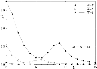
Figure 1: Variance of the logarithm of the stiffness as a function of $U$, for $W=2,5,9$ and for $M=N=14$.

In Fig. 1, the variance $\sigma^{2}$ is plotted as a function of $U$, for $M=N=14$. For $U=0$, the fluctuations are governed by the disorder and they increase when disorder increases. When interactions are introduced, fluctuations of two different natures compete. Figure 1 illustrates this by showing that these fluctuations compensate each other and decrease, phenomenon that leads to an increase in the magnitude of the persistent currents. Overall, this produces a maximum of magnitude for the persistent currents around $U\sim W/2\pm t$. For moderate $U$, the particles can move and two electrons can be together on the same site. Thus, the electrons explore sites with higher on-site potentials and under such conditions, the fluctuations are more sensitive to disorder. Finally, in the region where $U\lesssim W$, the variance increases. After this second maximum, the fluctuations decrease when the interaction increases for $U>W$. Within the region of very strong interactions, the particles are trapped alone within their sites and thus, their movement is frozen with exactly one particle per site. Fluctuations are on-site only and decrease systematically.

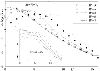
Figure 2: Dependency of the stiffness parameter upon the degree of interaction, for $M=N=14$ ($M=N=20$ in the inset), for disorders $W=0,2,5,9$. Lines represent individual samples. Symbols correspond to the global average. Error bars are smaller than the symbols size and hence, do not appear. Note that the curve for $W=0$ behaves as a Luttinger liquid.

Fig. 2 shows the dependency of the stiffness parameter $\log{D}$ on the degree of interaction, for $M=N=14,20$ for typical individual samples. These samples are represented by the single lines and global means are illustrated for three different disorder values, $W$, and for the clean case where $W=0$ (solid line). The ensemble averages of $\log{D}$ are performed over approximately 100 different samples (disorder realizations). The behavior of both the samples and the means are similar but in contradiction with the spinless fermions Dietmar01 . Indeed, our curves are all rather smooth ramin95 ; thierry95 even if small peaks appear for the individual samples for strong disorders ($W\sim 7,9$) in Fig. 2. This second peak increase of $\log{D}$ for samples occurs for $U\sim W-t$ when the fluctuations are strong (cf. Fig. 1). For $U=0$, the disorder leads to the Anderson localization and $\log{D}$ is strongly suppressed by increasing disorder lee85kramer93 . This is what would be expected in one dimension, for a non-interacting disordered system. For clean rings ($W=0$), the interaction always reduces the stiffness, which is consistent with a Luttinger liquid calculation loss92 ; stafford90 .

A weak repulsive interaction $U>0$ leads to an increase of the stiffness compared to its value for $U=0$, even when little disorder is present; such an increase was in fact predicted from a renormalization group approach, for both off half-filling and moderate disorders thierry95 . Indeed, the stiffness is less sensitive to disorder when repulsive interactions are accounted for than when attractive interactions only are considered, off half filling and for moderate disorders. This is clearly illustrated in Fig. 3, for an individual sample $M=N=10$. For attractive interactions no increase occurs and the stiffness phenomenon is strongly suppressed. The curves corresponding to different disorders do not cross to negative interactions, in accordance with the analytical development of Sec. III, which is valid only for positive interactions lieb93 .

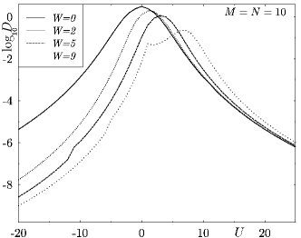
Figure 3: Dependency of the stiffness parameter for an individual sample upon the degree of interaction $U$, for $M=N=10$ and for disorders $W=0,2,5,9$. Interactions are both attractive and repulsive, $-20<U<25$. An increase occurs for positive interactions only.

At intermediate interaction levels i.e. for $U\in[t,W]$, the phase sensitivity exhibits a maximum around $W/2\pm t$, which becomes broader with increasing disorder. When disorder increases this maximum decreases, but the ratio $D_{\mathrm{m}ax}/D(0)$ is greater. With $M=N=14$, the mean ratios are equal to $1.4$, $8.1$ and $150$ for $W=2,5$ and $9$, respectively. These ratios are even greater for samples with $M=N=20$ and can under certain conditions be three times greater (e.g. for $W=9$).

For large repulsive interaction $U\gg W$, the behavior of $\log{D}$ is radically different. The stiffness decreases strongly with the degree of interaction and the numerical results confirm this with the analytical power law $\propto 1/U^{M-1}$, as illustrated in Fig. 4. The slopes for moderate interactions are stronger when the disorder strength W increases in order to recover the $1/U^{M-1}$ behavior when $U\gg W$.

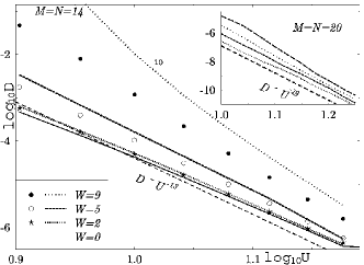
Figure 4: Data are plotted on log-log scale for $M=N=14$ ($M=N=20$ in the inset) under strong interaction conditions. Results confirm the power law $D\propto U^{-(M-1)}$. Symbols illustrate global means and lines individual samples.

Results for clean systems ($W=0$) and strong interactions gave the means to check a good concordance between observed results and the power law. This decrease is related to the localization due to the interaction loss92 . The most surprising result is that a curve crossing occurs within the Mott insulator limit (see Fig. 2) confirming that the disorder induces an increase in the stiffness parameter, as found analytically.

For all values of $U$ and $W$, we obtained negative $\Delta E$ for $M=N=6,10,14$, and positive $\Delta E$ for $M=N=20$. Thus, consistent with both Leggett’s rule Leggett for the non-interacting case and the analytical result for very strong interactions, the sign of $\Delta E$ is determined by the number of electrons that are each characterized by a given and specific spin, according to $(-1)^{N/2}$. Our numerical results revealed that this rule is valid for all tested samples and for all considered interaction and disorder values. In the following section, these results are compared to the phenomenon observed off half-filling.

IV Off Half-Filling

This section concerns systems off half-filling, $N\neq M$. The very strong interaction limit can be treated analytically and we maintain the notations presented in Sec. III. Details of the calculations are given in Appendix A.2. An example is developed in a toy model in Appendix A.3. The expansion is valid for an even number of particles and a single empty site, called a hole lieb93 ; tasaki95 .

Once again, we first consider the case without disorder. For very large $U$ the kinetic energy term $H_{K}$ represents a perturbation with respect to the dominating term $H_{U}$ as at half-filling tasaki95 . We must first determine the ground-state of the system. The basis-states are still given by eq. (9). Now since a hole has been introduced, the $\cal S$-states are connected by only one hop. A given basis-state $|\Psi_{\beta}\rangle$ can be connected to itself within an ensemble of first order hops, which are all going in the same direction to form a super-lattice nagaoka66 . For the toy model of two electrons on three sites of Appendix A.3, the number of super-lattices is equal to one. Increasing both the number of sites and the number of electrons increases the number of super-lattices and leads to the creation of $N/2$ subblocks, which is the number of electrons with the same spin present within the ring. We call these subblocks ${\cal C}_{i}$, where $i$ is the number of electrons of similar spin ones besides the others. Each subblock ${\cal C}_{i}$ leads to a different eigenvector, which implies that the ground-state degenerates. The basic structure of the ground-state can be determined by the standard Perron-Frobenius sign convention perronfrobenius in the case of a single empty site $N=M-1$. The ground-state is in such case a superposition of the $|\Psi_{\beta}^{{\cal C}_{i}}\rangle$ within each subblock ${\cal C}_{i}$. The sign of the weights depends on the boundary conditions tasaki95 ; lieb93 . If the transition amplitude between two states is negative, then one can superimpose within a subblock, states with the similar signs. Viceversa, if the transition is positive, one can superimpose states with opposite signs. These are in fact the Marshall sign rules marshall55 that are extended to the Hubbard model weng91 . The ground-state inside each subblock is written as:

$$|\Psi_{0}^{{\cal C}_{i}}\rangle=\sum_{\beta}f_{\beta}^{{\cal C}_{i}}|\Psi_{\beta}^{{\cal C}_{i}}\rangle\left\{\begin{tabular}[]{c}$f_{\beta}^{{\cal C}_{i}}>0$ for $\Phi=0$\\ $f_{\beta}^{{\cal C}_{i}}\in\Re$ for $\Phi=\pi$\end{tabular}\right.$$ (15)

where the weights $f_{\beta}$ are chosen to be real marshall55 ; perronfrobenius . Thus, for antiperiodic boundary conditions within each subblock ${\cal C}_{i}$, half of the basis-states will possess a positive (or negative) sign lieb93 ; tasaki95 . The first order corrections of the many-body ground-state energies are equal for periodic and antiperiodic boundary conditions. Indeed, in case of antiperiodic boundary conditions, each time an electron crosses the border, the sign due to the flux is compensated for by the sign of the weights. The phase sensitivity cancels out at first order. At second order, the intermediate states are obviously equal to $|\Psi_{\gamma}\rangle$’s, with exactly one doubly-occupied site. Lets now consider those sequences that cross the border. For example, that sequence where a particle jumps to form a doubly-occupied site and then, one of these electrons comes back to the initial site or jumps onto a neighboring site. These sequences are called exchange and double-jump. Their relative terms, when considering the two Hamiltonians, have opposite signs for periodic and antiperiodic boundary conditions. The eigenvalues for these matrices are different and hence, the phase sensitivity reads:

$$\Delta E^{(2)}= |E^{(2)}(0)-E^{(2)}(\pi)|$$

$$\Delta E^{(2)}= \frac{-t^{2}}{U}\kappa$$ (16)

where the factor $\frac{-t^{2}}{U}$ appears in all parts of both matrices. The phase sensitivity behaves as $1/U$ within the very strong interactions limit.

Now, if one introduces disorder, then the particles stay on the sites with the lowest disorder potentials inside each subblock ${\cal C}_{i}$ and form the ${\cal C}_{i}^{R}$-subspace. But one maintains $N/2$ subblocks. Hence, the ground-state is now a superposition of the basis-states ${\cal C}^{R}_{i}$ with the weights $f_{\beta}$ respecting the Marshall rule marshall55 ; perronfrobenius . A single jump does not lead to a basis-state anymore and one considers it now as two jumps. Under such conditions, the only possible sequences are the exchanges that lead to opposite values for periodic and antiperiodic boundary conditions. The phase sensitivity at second order here reads, after an expansion of $W/U$:

$$\Delta E^{(2)}=\frac{-2t^{2}}{U}\kappa^{\prime}(1+\frac{W^{2}}{U^{2}}d_{\alpha}^{2})$$ (17)

This $1/U$ power law is lower than at half-filling. Indeed, for $N=M$, the ground-state is rigid. When $N<M$, with the provided hole, the electrons can move more easily around the ring, which decreases the power law compared to the half-filled situation. This nicely illustrates the behavior of the persistent currents off half-filling under strong interaction limits. Electrons move around the ring without meeting each other and when close to the border, they hop on a doubly-occupied site. The phase sensitivity then decreases as the disorder strength $W$ increases. Unfortunately, the perturbation theory does not allow us here to conclude about the sign of $\Delta E$ under strong interaction limits.

We now present numerical simulations for $N=8$ particles ($4\uparrow;4\downarrow$) on $M=9$ and on $M=11$ sites. The symbols stand for the mean performance calculated over 100 disorder realizations (within a given sample); the lines represent individual samples. The results concentrate on an even number of electrons $N$, and we specifically consider the effect of the parity of the number of sites $M$. For an odd and an even value of $M$, the behavior of the stiffness is similar. Moreover, samples present similar behaviors as that observed for the mean curves. Finally, all curves are relatively smooth. The averages are calculated over the logarithm of the stiffness, $\log{D}$.

The variances for three values of the disorder $W=2,5,9$ are plotted as a function of the interaction for $N=8$ particles, for $M=9$ and $M=11$ sites. Results show that they are similar in Fig. 5.

Figure 5: Variance of the logarithm of the stiffness $\log{D}$ as a function of $U$ for different strengths of the disorder $W=2,5,9$ for $M=11$ ($M=9$ in the inset) and $N=8$.

For $0<U<W/2\pm t$, the behavior is similar to that expose in Sec. III, with the fluctuations that decrease. The persistent currents reach a maximum around $W/2\pm t$. Considering the strong interaction limits, the particles are trapped alone within their sites but a movement is still permitted because of the existence of an empty site (hole). The system is thus not rigid. Fluctuations are more significant than at half-filling since the fluctuations of both nature do not compensate, i.e. the on-site fluctuations and the fluctuations that are due to the disorder present on the empty site. When the disorder increases the fluctuations in the empty site increase, and so does $\sigma^{2}$.

In Fig. 6, the logarithm of the stiffness $\log{D}$ is plotted as a function of the interaction $U$, for different values of the disorder $W$ and for the clean case specifically.

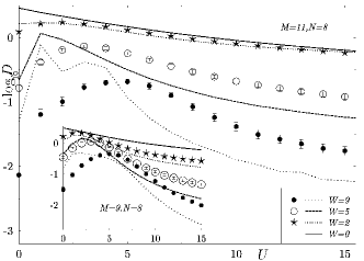
Figure 6: Dependency of the stiffness upon the degree of interaction $U$, for $N=8$, $M=11$ ($M=9$ in the inset) and $W=0,2,5,9$. Lines represent $\log{D}$ for individual samples and symbols correspond to global means.

At $U=0$ $\log{D}$ is strongly suppressed by the disorder (Anderson localization) lee85kramer93 . For clean rings, we verify that the interaction systematically reduces the stiffness, which is consistent with a Luttinger liquid calculation loss92 . A weak repulsive interaction leads to an increase of the stiffness respectively to its value in absence of interactions, as predicted by a renormalization group for moderate disorders thierry95 . We obtain this increase for all fillings and all non-zero disorder strengths. This increase can reach factors equal to approximately 1.5 (1.3), 4.5 (3.4), 28 (17) and when $W=2,5$ and $9$, respectively. This is true for the average system $M=11$ ($M=9$) and $N=8$. The increases of the samples are important and can reach an order of magnitude.

The stiffness $\log{D}$ decreases as the interaction $U$ increases, within the very strong interaction limits. Figure 7 presents the logarithm of the stiffness $\log D$ as a function of $\log U$ for $M=11$, $N=8$ and gives the means to determine that the power law follows $1/U$. We have verified that for the system $M=9$,$N=8$, the stiffness decreases as a function of $U^{-1}$, in agreement with strong interaction situations. For important disorder conditions, the slope must be calculated for interactions $U\gg W$ in order to recover the $1/U$ law.

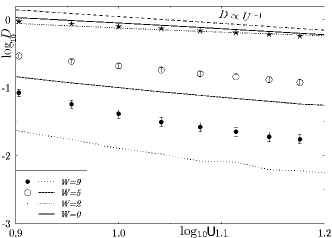
Figure 7: Data are plotted for strong interaction conditions in log-log scale for $M=11$ and $N=8$. They reveal a power law of $1/U$. The symbols represent means and the lines, individual samples.

This law is true for several holes even if the perturbation theory is valid only for single holes. In Fig. 8, the stiffness is smaller for negative interaction values than for positive ones thierry95 , and no stiffness increase occurs.

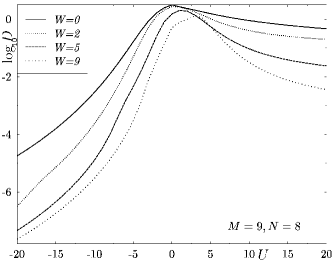
Figure 8: Illustration of the behavior of $\log D$ for a sample of $M=9$ sites and $N=8$ electrons for negative and positive interactions $-20<U<20$. Note that an increase occurs for positive interactions only.

The sign of the phase sensitivity was also studied and results demonstrate that it also follows the Leggett’s rules Leggett . The sign depends on the number of electrons that possess a specific spin, according to $(-1)^{N/2}$. This was observed for all disorder and interaction values. The present result was verified numerically for all the computed samples. For $N=8$, the phase sensitivity is always positive and for $N=6$ the phase sensitivity is negative, whatever the number $M$ of sites.

V Role of the spin

The logarithm of $D$ gave us the means to model the behavior of the persistent currents as a function of $U$, for different values of the disorder $W$ and for different system sizes $M$. Our conclusion is that a pronounced increase occurs for all degrees of disorder not equal to zero, for every system size $M$ and arbitrary fillings, but for moderate values of the interaction $U\sim W/2$.

This increase can be explained through the competition between disorder and interaction phenomenon. Indeed, the disorder sets the electrons within the sites with the lowest potentials whereas the interaction sets a unique electron per site. When disorder and interaction are of the same strength, the determination of the ground-state of the system is difficult. Indeed, the electrons oscillate between being together on the same site hence, adding an energy level to $U$ or being on two different sites which sets a different degree of disorder, energy $Wv_{i}$. However, the ground-states directly depend on the spin parameter, where the case of half-filling corresponds to $M=N$. When $W>U$, electrons may prefer avoiding the site with highest potentials and hence, will generate a doubly-occupied site (a spin up and a spin down). When $U$ and $W$ are of the same order, the electrons move easily as the doubly-occupied site can hop freely around the ring and set itself next to the site with the highest potential. Under such conditions, if $W\sim U$, a particle from the doubly-occupied site can jump on the site and further on to its neighbor, recreating a doubly-occupied site. The quantity here important to consider is the difference, $U-W/2$. When it is smaller than the amplitude transition $t$, the electrons movement around the ring is easy and induces an important current. This behavior can be related to calculations for 2D spinless fermions with disorder and long range Coulomb interaction benenti99 . When $W<U$, the particles remain alone on their respective sites and this leads to a decrease in the magnitude of the current. For off half-filling, this explanation is also valid but the holes are placed upon the highest disorder potentials. Hence, the maximum current further decreases. This simple mechanism of two competing ground-states is a starting point for a better understanding of what happens in two dimensions, and provides a starting indication of how persistent currents may be enhanced by large orders of magnitudes.

We illustrate this modeling considering first a very weak disorder $W=0.1$, for the two following systems $M=N=10$, and $N=8$, $M=11$. Here $\log{D}$ is calculated from a group average of about 100 samples. An increase is already observable for such a weak disorder in Fig. 9. One can see that a maximum increase is obtained for $U\sim 0.05=W/2$.

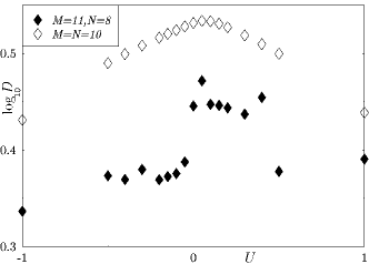
Figure 9: Interaction dependency of the stiffness parameter on the degree of interaction, for $W=0.1$ in the case of two systems, $M=N=10$ and $N=8$,$M=11$. These results are calculated from a group average of 100 samples.

These results give us the means to conclude to an increase of the stiffness for non-vanishing disorders. The persistent currents are less important for $M=11$, $N=8$ than for $M=N=10$.

For negative interactions, the stiffness always decreases. Indeed, two electrons with opposite spin directions can both generate a doubly-occupied site and be on the sites with lowest potentials. This decreases the stiffness as soon as $U<0$ for all disorders strengths, as found in Fig. 9.

In Fig. 10, a sample of $N=4$ electrons on $M=13$ sites is presented in order to show that even for low fillings i.e. $(N/M)\sim 0.3$, persistent currents increase. This increase reaches an order of magnitude for moderate ($W=5$) and strong ($W=9$) degrees of disorder.

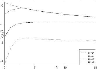
Figure 10: $\log{D}$ is plotted as a function of $U$, for different values of the degree of disorder $W$, for an individual sample of $N=4$ electrons present on $M=13$ sites.

Thus, the mechanism that have been presented above to explain the increase of the persistent current is valid even for low fillings and for attractive and repulsive interactions in presence of disorder. Other studies have previously considered the role of the spin and have also concluded that it is an important parameter for both one and two dimension situations, and for multi-channelled systems georges94b . The present work shows in addition that in one dimension, the spin has a significant influence on the magnitude of the persistent currents.

In the previous sections (III and IV), the limit for the strong interactions revealed different behaviors for half-filled and non half-filled systems.

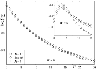
Figure 11: $\log{D}$ is illustrated as a function of $U$, for $W=0$ ($W=5$ in the inset) for systems with $N=8$ and $M=9,10$ or $11$. A significant crossing between the curves is observed for strong interactions.

We now consider the case of a similar number of particles and a similar degree of disorder (even $W=0$) but with different filling properties (i.e. not equal to 0.5). For strong interactions i.e. when the filling decreases for a given number of electrons, the stiffness increases. This is illustrated in Fig. 11. The presence of holes makes the persistent currents increase within the strong interaction limit. The case of half-filling deserves to be treated apart and presents a different behavior, which underlines the important effect of the particle-hole symmetry for the electrons denteneer01 .

VI Localization Length

In this final section, we study the localization length $\xi$ in order to characterize the finite-size effect lee85kramer93 . In order to extract $\xi$, we use a relation that is valid for localized systems. The localization length is related to the stiffness $D$ through:

$$\ln{D}=\ln{(A(U))}-M/\xi(U).$$ (18)

$\log{D}$ is plotted as a function of $M$ and one must check that a straight line is obtained. Thanks to a linear regression the slope, which is proportional to $1/\xi(U)$ can be obtained from the numerical data of $\log{D}$, indicated here by the dimension of the error bars. This relation is phenomenological and is obtained thanks to dimensional reasoning but does not allow for the determination of the sign.

VI.1 Localization length at half-filling

Disordered non-interacting one-dimensional systems are Anderson insulators lee85kramer93 , whereas a half-filled system behaves as a Mott insulator for very strong interactions Mott . We consider half-filled rings $M=N=6,10,14$. We first verified the results obtained for $W=0$. First, plots representing $\log{D(M)}$ must be straight. For $U=W=0$, a free electron gas is obtained and the localization length should both diverge and be infinite. Because of the numerical errors, one gets a very high finite value of the localization length $\xi$. Once the interaction is introduced, $\xi$ can be extracted. It decreases as a function of the interaction increase (see Fig. 12). This has previously been reported stafford90 .

Figure 12: $\xi$ is plotted as a function of $U$, for $W=0$. The symbols represent the values of $\xi$ obtained from $\log{D}$. In the bottom inset, $\xi\Delta$ LiebWu is presented as a function of the interaction $U$, for $3<U<8$. In the top inset, $\xi^{-1}$ behaves according to the Bethe Ansatz within the strong interaction limits stafford90 .

For moderate interactions, $U\in[3,8]$, the quantity $\xi\Delta$ ($\Delta=\frac{8t^{2}}{U}\int_{1}^{\infty}\frac{\sqrt{(y^{2}-1)}dy}{\sinh(2\pi ty/U)}$, the Lieb-Wu charge gap LiebWu ) must reach the mean-field result of $(\xi\Delta)/t=4$ stafford90 . The values calculated thanks to our numerical approach reached 4.9, for $U=0$ (see the bottom inset of Fig. 12). For very strong interactions the inverse of the localization length behaves as the analytical solution given by the Bethe Ansatz stafford90 . This is in agreement with what was presented in Sec. III. The inverse of the localization length $\xi^{-1}$ (see the top inset of Fig. 12) behaves as $-1.49+\ln{U}$ for $W=0$.

We want to study the influence of the competition between disorder and interaction on the localization length $\xi$. The inverse of $\xi$ is represented in Fig. 13 as a function of $\ln{U}$, for different strengths of the disorder $W$. The inset presents $\log{D(M)}$ for $U=1,W=2$. The $U=0$ limit shows that $\xi$ decreases when the disorder increases as for the Anderson localization. For moderate interactions, an enhancement of the localization length $\xi$ when compared to its non-interacting value is observed for all disorder strengths $W$. The values for $W=2$ are very high, even larger than the sizes of the studied systems. In such a case, eq. (18) is not valid anymore. Yet, it is possible to conclude to a strong and significant increase of $\xi$. The increase factors $\xi_{{\rm max}}/\xi(U=0)$ reaches 2.2, 3.4 and 4.5, for $W=2,5$ and $9$, respectively. They are significant and confirm the delocalizing effect. The maximum of $\xi(U,W)$ belongs to the interval $[\frac{W}{2}\pm t]$ and decreases as $W$ increases. This strong enhancement suggests that the wave functions are less localized and that the electrons might move more easily on several sites. Moreover, the stiffness depends on the localization length according to the equation: $D(M)=(-1)^{M/2+1}M^{1/2}D(U,W)\exp{-M/\xi(U,W)}$ stafford92 . Hence, when $\xi$ increases, $D$ also increases and the persistent currents will consequently increase even for large finite rings of circumference $M$. Another weak increase for the localization length had been reported for spinless fermions but only for a strong degree of disorder rodolfo01 . In the case of strong interactions, the localization length $\xi$ decreases with increasing $U$, as a Mott insulator. As for the stiffness $D$ that was presented in Sec. III close to the strong interaction limits, the disorder phenomenon has the unexpected effect of increasing the localization length. This phenomena that is observed for systems of $M=20$ sites can be extended to bigger systems.

In order to illustrate both competing regimes, one should fit the inverse of the localization length. Fig. 13 shows that $\xi^{-1}$ depends on $\ln{U/t}$ for all disorder strength.

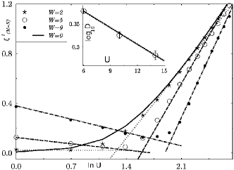
Figure 13: $\xi^{-1}(M=N)$ is plotted in function of $\ln{U}$. The dotted lines represent the fitting of both regimes for $W=2,5$ and $9$.

This dependence is expected for very strong interactions and $W=0$ stafford92 . However, for $W\neq 0$ and for weak interactions, the inverse of the localization length behaves like $\ln{U^{-|a|}}$ as a correlation length whereas for strong interactions it behaves following $\ln{U^{+|b|}}$. For example when $W=2$, $\xi^{-1}$ behaves as $-1.0+0.8\ln{U}$ for weak interactions and then, as $0.022-0.001\ln{U}$ for strong interactions, in Fig. 13. In Fig. 14, $\log{D}$ is represented as a function of $\ln{U}$ and two different regimes also clearly appear. First $D$ increases up to $U^{+|a^{\prime}|}$ and then decreases up to $U^{+|b^{\prime}|}$. This is true for all the systems that we considered as well as for all non-zero disorders.

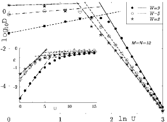
Figure 14: $\log{D}$ ($\epsilon$) is plotted as a function of $\ln{U}$ ($U$) for half-filled systems for $W=2,5,9$. The dotted lines are the fitting for both regimes.

The energy density $\epsilon=\partial E/\partial M$ was represented as a function of the interaction $U$, for different disorder strengths $W=2,5,9$ (see inset of Fig. 14). At half-filling, when $U$ is strong, the particles tend to stay isolated within their site and the system becomes rigid, as previously mentioned in Sec. III. The energies converge towards zero, and the density of energy increases as $-\exp{-CU}\sim CU$. For very strong interactions i.e. when there is exactly one particle per site, there is little displacement and the energies correspond to the total sum of the on-site potentials. As the systems are half-filled and the potentials are random, the sum tends to converge to zero for all degrees of disorder. The energy density tends to saturate at zero. Thus, one fits $\epsilon$ for weak and strong interactions with straight lines proportional to $U$.

Figures 13 and 14 present the two competing regimes and reveal a very sharp crossover, as the fittings joining at $U_{\mathrm{cross}}$ covers almost the totally of the symbols used in the different curves. Here, we illustrate two exclusion limits. For $U=0$, the electrons with opposite spin remain on the same site (Pauli principle) while for infinite interactions, the electrons avoid being on the same site (the exclusion principle). For strong interactions, the mobility of the electrons is weak since they are trapped alone within their site and hence, the movement is frozen. When the interaction reduces, electrons can jump on other sites and the crossover can then occur. For weak interactions, the electrons can move easily on multiple sites and the movement is dominated by quantum fluctuations. The second derivative of the quantities $\xi^{-1}$, $\log{D}$ and $\epsilon$ illustrate this crossover. For weak interactions, $\partial^{2}\epsilon/\partial U^{2}$ behaves as $-C^{2}\exp{-CU}$ while for strong $U$, it is a constant. Between these limits, a peak exists and symbolizes the crossover. A study of the shift for this peak as a function of the degree of disorder should be considered to describe the corresponding crossover as a function of the interaction, $U_{\mathrm{cross}}$ as shown in Fig. 18.

VI.2 Localization length off half-filling

The study of the localization length is now considered for off half-filling. One considers three systems with a similar number of particles $N=8$, but with different size $M=9,10,11$. Some of these systems were presented in Sec. IV.

Fig. 15 illustrates $\log{D(M)}$ for different degrees of interaction, with $W=5$. As in Fig. 11, results reveal that for $U>W$, $\log{D(M)}$ increases as $M$ increases. The slope is thus positive. This leads to a change in the sign of the localization length off half-filling which is in agreement with the comments made following eq. (18).

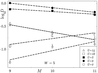
Figure 15: $\log{D}$ is plotted as a function of $M=9,10,11$ for a degree of disorder $W=5$, for $N=8$ particles. The slope of $\log{D}$ changes sign as $U$ increases.

One can assume that approximately straight lines are present even if only three points are here considered. At the point where the curves $\log{D(U,M)}$ cross (see Fig. 11), the localization length strongly increases and reaches a high positive value. After the crossing, it reaches an important negative value before increasing once more. Figure 16 illustrates this behavior for $W=0,2,5,9$, considering the inverse of the localization length $\xi^{-1}$. When $U=W=0$, the localization length starts at a very high value and decreases when $U$ increases. When $U=0$, $\xi$ decreases as the degree of the disorder increases as it is case for the Anderson insulator lee85kramer93 . For $W=0$, $\xi$ decreases, then, a change in sign occurs and $\xi$ increases up to a disorder-dependent negative value. For all disorders $W\neq 0$ and moderate values of $U$, $\xi$ increases strongly compared to its non-interacting value. If one considers the positive values of $\xi$, it is noticeable that $\xi(0)>\xi(2)>\xi(5)>\xi(9)$ (except for $U=2$, due to numerical errors). If the highest positive value is not considered, the ratios $\xi_{\mathrm{max}}/\xi(0)$ reach 1.5, 2.75, and 4 for $W=2,5$ and $9$, respectively. These ratios are close to but smaller than those observed at half-filling. After the change in sign, the localization length increases up to a negative value $\xi_{\mathrm{neg}}$ that depends on the degree of disorder. When the disorder increases, the localization length decreases as expected for off half-filling (Sec. IV).

In order to study both regimes (Pauli and exclusion limits) as was in Sec. VI.1 one fits $\xi^{-1}$ as a function of $\ln{U}$ for weak and strong interactions in order to obtain the $U_{\mathrm{cross}}$. This is presented in Fig. 13.

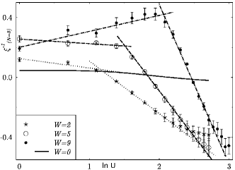
Figure 16: $\xi^{-1}$ is plotted as a function of $\ln{U}$ for $W=0,2,5,9$, for $N=8$ particles. The straight lines correspond to the fits of both regimes. A crossover is here identified.

For positive values, the inverse of the localization length $\xi^{-1}$ behaves as $\ln{U^{-|a_{2}|}}$ and for strong interactions, the localization length behaves as $\ln{U^{-|b_{2}|}}$ because of the change in sign. In Fig. 17, the curves plotting $\log{D}$ as a function of $\ln{U}$, for various degrees of disorders, are represented and it is possible to fit them with lines proportional to $\ln{U}$. They present behavior similar to that observed for half-filling behaviors.

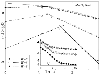
Figure 17: $\log{D}$ ($\epsilon$) is plotted as a function of $\ln{U}$ ($U$) for $N=8$. The dotted lines correspond to the fitting of both studied regimes.

The energy density $\epsilon=\partial E/\partial N$ is represented as a function of the interaction $U$, in the inset of Fig. 17. For weak interactions, the electrons are placed by pairs (with opposite spin directions) within the same site. In addition, the corresponding energies are summed over $N/2$ sites. When the interactions become stronger, the energies increase as it would be the case for sums over less negative potentials. The energies of the ground-state when the number of sites increases, decrease strongly. This leads to a decrease in the energy density as expressed by $\exp{-CU}\sim-CU$. For very strong interactions, the ground-state energies are summed over on-site potentials. As there are empty sites, the energy density tends to saturate at a specific negative value that increases with the strength of the disorder.

The quantities $\epsilon$, $D$ and $\xi$ highlight the presence of a crossover as mentioned in Sec. VI.1 and gives the means to determine the existence of a peak between the two different regimes. The position of the peak is given by the value $U_{\mathrm{cross}}$, when the curves fitting both regimes cross.

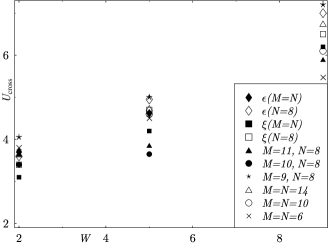
Figure 18: $U_{\mathrm{cross}}$ as a function of the disorder $W$ for systems at and off half-filling.

In Fig. 18, the movement of the peaks is a function of the strength of the disorder $W$, for systems at and off half-filling. When $W$ increases, the interaction must be stronger in order to reach the second regime where the particles will be localized alone within their site. The peaks and hence, the crossovers occur quickly around the same value of the interaction $U$, for a given disorder $W$. This is true for all systems. The values of $U_{\mathrm{cross}}$ are very close but more scattered for off half-filling. The competition between the two regimes that are represented by the Anderson and the Mott insulators is very important in order to gain a better understanding of the two dimensional metal-insulator transition, which is at the heart of the problems in mesoscopic physics kravchenko94 . With disorder only, no metal-insulator transition is found lee85kramer93 . When including these interactions, it is possible to determine two different regimes in one dimension. This may explain the metal-insulator transition in two dimension situation.

VII Conclusion

We investigated the effect of electron-electron on-site interactions on the persistent currents found in disordered one-dimensional rings with arbitrary fillings. We took into account the spin and considered the stiffness as a measure of the magnitude of the persistent currents. Our numerical simulations indicate a strong increase in the stiffness with respect to the non-interacting case observed for moderate interactions and arbitrary fillings. This strong enhancement, which is also observed at the level of disordered realization, can be attributed to the mechanism of both competing forces, i.e. disorder and interaction. A simple computation comparing the weakly interacting state systems in the presence of disorder shows an increase in the electrons mobility within the ring. The stiffness decreases for stronger interactions according to a power law that is different at and off half-filling. The analytical approaches helped us to determine the power laws for both cases. An unexpected behavior was also observed at the strong interaction limit, specifically at half-filling: the disorder rendered the stiffness stronger. Such an effect can be explained by the disorder-induced reduction in the energy gap between the Mott insulator ground-state and the excited states. By studying the localization length, we here further observed that the interactions increase the persistent currents even for a large finite size of rings at half-filling. The localization length, which is defined phenomenologically, changes sign off half-filling. The behavior of the energy density, the stiffness as well as the localization length suggest a crossover between weak and strong interactions. Based on these results, we can conclude that the spin plays a significant role and influences the increase in magnitude of persistent currents.

Appendix A Perturbation expansions

A.1 Half-filling

We give here the details for the analytical approach in Sec. III. The ground-state is given by eq. (11) for both periodic and antiperiodic conditions lieb62 ; lieb93 . The aim here was to define sequences (the set of hops defined in Sec. III) that may lead to discrepancies within the corrections brought to the energy level.

The terms presented in the numerator of $E^{(n)}$ are equal to $-t$ but the signs of the permutations of the electrons, with spin up or down, could be negative as the hopping element changed the electrons order. For periodic boundary conditions, the numerator can be written as $N_{p}=(-t)^{n}\mathrm{sign}(P_{\uparrow})\mathrm{sign}(P_{\downarrow})$ where we define $P_{{\uparrow}({\downarrow})}({\bf A})$ $\uparrow$($\downarrow$) as the permutation of the positions for up (or down) electrons around the ring, which is a resultant from the defined sequence ${\bf A}$. Since the flux appears only within the kinetic part $H_{K}$ of the Hamiltonian, a unique change only appears when a particle crosses the border for antiperiodic boundary conditions. This introduces a sign $(-1)$ in the numerator. Thus, the numerator for antiperiodic boundary conditions is equal to : $N_{ap}=(-1)^{h_{b}}~{}N_{p}$ where $h_{b}$ is the number of hops across the border $1~{}\longleftrightarrow~{}M$ contained in ${\bf A}$. For orders lower than $M$, the $n^{\rm th}$ order energy is a constant in $\Phi$ that does not depend on the boundary conditions and the phase sensitivity is zero. Indeed, an even number of hops is needed to recover one of the eigenstates and in this case, the border is crossed twice. To obtain a difference, the particles must circulate around the ring and the lowest contributions are of order $M$; in such case, a particle crosses the boundary condition only once. Our work gave us the means to define different sequences connecting two basis-states, $|\Psi_{\beta}\rangle$ and $|\Psi_{\beta}^{\prime}\rangle$, and to obtain eq. (III). These sequences have previously been published gambetti02 .

When disorder is reintroduced, the perturbation theory remains second order, with an exchange energy that is now equal to $\frac{2t^{2}}{U(1-\frac{W^{2}}{U^{2}}(v_{i}-v_{i-1}))^{2}}$. The matrix elements of the Hamiltonian are under such conditions even-functions of $\frac{W}{U}$, so are the weights $f_{\beta}$. They read: $f_{\beta}\approx f_{\beta}^{(0)}+f_{\beta}^{(2)}(\frac{W}{U})^{2}$. In the following development, we maintained $f_{\beta}^{(0)}$ only and $f_{\beta}\sim f_{\beta}^{(0)}$ was approximated. In order to study the effect of disorder on the phase sensitivity for strong interactions ($U\gg W$), we expand the denominator under powers of $W/U$. When second order is reached, this yields :

$$\Delta E^{(M)}\approx\frac{(-1)^{N/2}4t^{M}}{U^{M-1}}\sum_{\beta,\beta^{\prime}}\sum\limits_{{\bf A}_{\rm f}^{(\beta,\beta^{\prime})}}\frac{f_{\beta}f_{\beta^{\prime}}}{\prod_{l}g_{\gamma_{l}}}$$

$$\left(1-\frac{W}{U}\sum_{l}\frac{d_{\gamma_{l}}}{g_{\gamma_{l}}}+\frac{W^{2}}{U^{2}}\left(\sum_{l}\frac{d_{\gamma_{l}}^{2}}{g_{\gamma_{l}}^{2}}+\sum_{l<m}\frac{d_{\gamma_{l}}d_{\gamma_{m}}}{g_{\gamma_{l}}g_{\gamma_{m}}}\right)\right).$$ (19)

The dominating term of (A.1) corresponds to the power law found in section III. We now consider the term of the first order in $W/U$ and this first-order correction for $W/U$ vanishes because of the particle-hole symmetry. Indeed, if one characterizes a given sequence of hoppings by the positions of the doubly-occupied and the empty sites, one can always construct moving the particle along the ring a second sequence by exchanging the places of the doubly-occupied and the empty sites. These two sequences will possess an equal number of doubly-occupied sites $g_{\gamma_{l}}$ and their coefficients $d_{\gamma_{l}}$ will have opposite signs. This first order term vanishes when the sum over all the sequences is taken. Thus, the second order term of (A.1) determines the disorder dependence of the persistent current for $U\gg W$. The first term is of order $1$ and is always positive. Hence, for each sequence the sum over positive quantities of order one only are taken and it is possible to estimate: $\sum_{l}(\frac{d_{\gamma_{l}}}{\epsilon_{\gamma_{l}}})^{2}\lesssim M$. By summing over all the sequences, we obtain a positive term of order $N_{S}M$. The second term is also of order $1$ but has a random sign. Taking the sum over all sequences, it is evaluate to almost $\frac{\pm\sqrt{N_{S}M}}{\sqrt{2}}$. Since the number of sequences is very high, one obtains $\sqrt{N_{S}}\ll N_{S}$. This results in eq. (III). It is concluded here that the phase sensitivity possesses positive corrections of order $(\frac{W}{U})^{2}$, so does the stiffness $D$.

A.2 Off half-filling

We give here the details of the calculations for the perturbation expansion that was presented in section IV. The ground-state is given by eq. (15).

The matrix element of second order contains intermediate states with exactly one doubly-occupied site, $|\psi_{\gamma}\rangle$’s, that connect $|\psi_{\beta}^{{\cal C}_{i}}\rangle$ to $|\psi_{\beta}^{{\cal C}_{j}}\rangle$, as the second jump leads to $|\Psi_{\beta}\rangle$. We seek to develop sequences of two jumps that will lead to different terms ${\cal H}^{(i,j)}$, according to the defined boundary conditions. Then, crossing border sequences are considered. The first sequences are the exchange sequences, where two electrons exchange places with one another, across the border, as illustrated in Fig. 19. Under such conditions and for both periodic and antiperiodic boundary conditions, the factor $F=\langle\psi_{\beta}^{{\cal C}_{i}}|H_{K}|\psi_{\gamma}\rangle\langle\psi_{\gamma}|H_{K}|\psi_{\beta}^{{\cal C}_{j}}\rangle$ is equal to $t^{2}$. More specifically, under periodic boundary conditions, weights have equal signs, whereas under antiperiodic boundary conditions, weights have opposite signs because of the Marshall’s rules weng91 ; marshall55 . A second type of sequence, called the double jump is illustrated in Fig. 19, and brings different terms ${\cal H}^{(i,j)}$ to the Hamiltonians. Under periodic and antiperiodic boundary conditions, the factor $F$ is equal to $t^{2}$ and $-t^{2}$, respectively. In addition, under periodic boundary conditions, weights maintain equal signs. However, under antiperiodic boundary conditions, the double jump is equivalent to two hops for a given particle i.e. equivalent to a change in sign and an exchange. This is also illustrated in Fig. 19. Overall, this second type of sequence gives an end product with an equal sign for the weights of both $f_{\beta}^{{\cal C}_{i}}$ and $f_{\beta}^{{\cal C}_{j}}$.

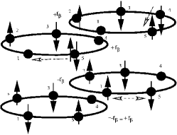
Figure 19: Example of a “double jump” sequence for $M=5$ and $N=4$. The third and fourth drawing illustrates an ”exchange” sequence.

This leads to a contribution of a second order phase-sensitivity. The factorization of $-t^{2}/U$ for all the different terms of both Hamiltonians leads to eq. (IV).

When disorder is introduced, the ground-state is a superposition of the basis-states within each subspace ${\cal C}^{R}_{i}$ with weights $f_{\beta}$ chosen to be real. At this point, one assumes that the Marshall rule is still valid in presence of disorder marshall55 ; perronfrobenius . Due to signs of the weights, the only possible sequences that could lead to opposite values for periodic and antiperiodic boundary conditions are the exchange sequences. Now, using sums over two-hops sequences ${\bf A}^{(\beta,\beta^{\prime})}$, the second-order phase sensitivity reads:

$$\Delta E^{(2)}=\frac{-2t^{2}}{U}.\frac{\kappa^{\prime}}{(1-\frac{W^{2}}{U^{2}}d^{2}_{\gamma})}$$ (20)

The expansion of eq. (20) leads to the eq. (17).

A.3 Toy model

The toy model is presented here to help explain the stiffness behavior that was presented in Sec. IV, for general systems of $N$ electrons on $M$ sites. Here, we consider a simplified model of two electrons for three sites. Such a model was studied by H. Tasaki and provided the means to verify parts of our results tasaki95 . This small system is described by the Hubbard-Anderson Hamiltonian of eq. (1), when restricted to three sites. In this case, one considers one empty site only tasaki95 ; lieb93 , as Sec. IV.

We first use numerical manipulations in order to compute the many-body ground-state energies and to deduce the phase sensitivity. The basis-states are given by eq. (9). Thus, diagonalization of the matrices is necessary to obtain the eigenstates for all values of the parameters $t$, $U$ and $v_{i}$. The case without disorder is now considered. Under periodic boundary conditions, the energy level is described by $E(0)=\frac{1}{2}U-t-\frac{1}{2}\sqrt{U^{2}+4Ut+36t^{2}}$. As far as the antiperiodic conditions are concerned, the minor eigenvalue is equal to $E(\pi)=-2t$. Now it is possible to calculate, using eq. (7), the contributions to the phase sensitivity. This would lead to:

$$\Delta E= E(0)-E(\pi)$$ (21)

$$=t+\frac{1}{2}U-\frac{1}{2}\sqrt{(U^{2}+4Ut+36t^{2})}$$

For very strong interactions, an expansion in $t/U$ can be performed and the phase sensitivity is then given by:

$$\Delta E\approx-\frac{8t^{2}}{U}$$ (22)

This quantity behaves as $1/U$ and decreases when $U$ increases. For periodic boundary conditions, the ground-state of the system is a superposition of the states $|\Psi_{\beta}\rangle$ and $|\Psi_{\gamma}\rangle$. All weights are positive. Indeed, the unnormalized weights for the states $|\Psi_{\beta}\rangle$ are all equal to one whereas those for the states $|\Psi_{\gamma}\rangle$ are equal to $f^{*}_{\gamma}$. One assumes ${\cal N}^{2}=3(f^{*}_{\gamma})^{2}+6$. The components of the $|\Psi_{\gamma}\rangle$’s are written as follows:

$$f_{\gamma}=\frac{f^{*}_{\gamma}}{\cal N}=-\frac{1}{2}\frac{\frac{1}{2}U+t-\frac{1}{2}\sqrt{U^{2}+4tU+36t^{2}}}{t{\cal N}}$$ (23)

The development of these weights $f_{\gamma}$ for very large $U$ is such that (see eq. (24)):

$$f_{\gamma}\approx\frac{8t}{2U\cal N}.$$ (24)

The weights of the $|\Psi_{\gamma}\rangle$’s decrease down to zero whereas the weights of the states $|\Psi_{\beta}\rangle$ are equal to

$$f_{\beta}=\frac{1}{\cal N}\approx\frac{1}{\sqrt{6}}.$$ (25)

We consider that for the ground-state and within the limits of very strong interactions, one can neglect these $|\Psi_{\gamma}\rangle$’s. Under antiperiodic boundary conditions, the corresponding eigenvector is the superposition of the $|\Psi_{\beta}\rangle$’s with alternated signs.

Second, it is possible to calculate the corrections to bring to the energy level using the perturbation theory in order to recover the values of the phase sensitivity given by eq. (22). The basis-states remain the $\cal S$-states. The first state has an $\uparrow$-electron on the first site and a $\downarrow$-electron on the second site, the last site being empty in all cases. The other states are generated by one hop processes. This set of six states constitutes a ”super-lattice” nagaoka66 and is a good illustration of the connectivity condition tasaki95 . The basic structure of the ground-state is determined following the Perron-Frobenius sign convention tasaki95 ; lieb93 ; perronfrobenius . The ground-states are in fact the superposition of the six states, denoted $|1\rangle\cdots|6\rangle$, with signs respecting the Marshall’s rule marshall55 as indicated in the following:

$$|\Psi_{0,\Phi=0(\Phi=\pi)}\rangle=\frac{1}{\sqrt{6}}$$

$$\left(|1\rangle+|2\rangle+|3\rangle+\left(-\right)|4\rangle+\left(-\right)|5\rangle+\left(-\right)|6\rangle\right)$$ (26)

We can now calculate the periodic and antiperiodic many-body first-order energies levels. Under periodic boundary conditions, each $|\psi_{\beta}\rangle$ is coupled to two other states by a single jump, and all terms are positive $E(0)=\frac{1}{6}(-t)\times 2\times 6=-2t$. Under antiperiodic boundary conditions, the negative sign that is induced by the flux, is compensated by the negative sign of the weights each time the electron crosses the border line. One gets $E(\pi)=-2t$. This result shows that the phase sensitivity cancels at first order, as explained in Sec. IV. Similar eigenvalues are obtained through the numerical diagonalizing of the matrices that are formed with the basis-states $|1\rangle\cdots|6\rangle$. The calculations must be increased to the second order in order to recover a contribution. Hence, one must consider two-hops sequences across the border. The first jump leads to a doubly-occupied site whereas the second jump leads to one of the many basis-states. Each state $|i\rangle~{}(i=1,\ldots,6)$ is connected to two states $|\Psi_{\gamma}\rangle$. Each of these $|\Psi_{\gamma}\rangle$’s can lead to 4 different $|\Psi_{\beta}\rangle$’s. Under periodic boundary conditions, since the weights are equal and posses similar signs, the contribution is $E^{(2)}(0)=\frac{1}{6U}[6\times 2\times 4\times(-t^{2})]=-8t^{2}/U$. In the case of antiperiodic conditions, the sum over these terms cancels out. Indeed, if we now consider the state $|1\rangle$, half of the terms contain a negative sign and the other half a positive one and hence, the contribution is zero. A similar comment can be given to other states, thus, the phase sensitivity is equal to $-8t^{2}/U$ as was obtained in eq. (22). This confirms the validity of the perturbation theory within the limit for very strong interactions.

In this toy model one introduces a disorder $v$ on the first site, when considering the limits for very strong interactions. The $6*6$ matrix can be diagonalized with the disorder $v$ placed upon the first site. This yields :

$$E_{{\rm periodic}}=E_{{\rm antiperiodic}}=\frac{(E(v)+E(-v))}{2}$$

$$=\frac{1}{2}t-\frac{1}{4}\sqrt{v^{2}-2tv+9t^{2}}-\frac{1}{4}\sqrt{v^{2}+2tv+9t^{2}}.$$ (27)

Even in the presence of disorder, the first-order phase sensitivity is equal to zero. Hence, for strong disorders, particles occupy the disordered states associated to the following weight:

$$f_{\beta}= \frac{\frac{1}{2}v-\frac{1}{2}t-\frac{1}{2}\sqrt{v^{2}-2tv+9t^{2}}}{t{\cal N}^{\prime}} \approx_{v\to\infty}\frac{9t^{2}}{4v{\cal N}^{\prime}}$$ (28)

where $({\cal N}^{\prime})^{2}=\sum_{\beta}(f^{*}_{\beta})^{2}$. The $f_{\beta}(W\to\infty)$ decrease when $W$ increases. This gives the means to avoid the sites with highest potentials in Sec. IV.

Appendix B Very strong interactions limit

This part concerns the infinite interaction case. The ground-state components at half-filling were considered. A program was developed in order to calculate the weights of the eigenvectors when two particles can not remain together upon the same site ($U\to\infty$). We computed the weights of each component for the ground-state as a function of the ring size $M$, for $M\in[2,14]$. The most significant weights, $f_{\mathrm{alt}}$, are those of the states with alternated spins; the second most important ones, $f_{\mathrm{max2}}$, correspond to states where two electrons have exchanged their positions when compared to the states with alternated spins. We have represented the logarithm of these $f_{\mathrm{alt}}$ and $f_{\mathrm{max2}}$ weights as a function of the size of the system $M$ (see Fig. 20). It was established that the weights $f(M)$ can be fitted by an exponential. This result gave the means to extrapolate what would be obtained in the case of large $N$: we speculate that for big systems, the alternated spin configurations will be the most significant contributor to the phase sensitivity parameter. Moreover, as the ratio $R$ saturates and as soon as $M\geq 12$, one may conclude that the corrections brought to the phase sensitivity will essentially depend on both $f_{\mathrm{alt}}$ and $f_{\mathrm{max2}}$ weights. Here, the particles move easily around the ring, especially for the states with alternated spins. Consequently, an important current may be induced.

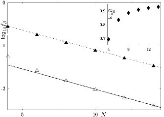
Figure 20: Logarithm of the most significant components for the ground-state of half-filled systems ($N=M$) (in the inset is presented the logarithm of their ratio $R=f_{\mathrm{alt}}/f_{\mathrm{max2}}$) for infinite interactions as a function of the system size, $M$.

Appendix C Odd number of electrons

Here, we consider the rings filled with an odd number of electrons. The behavior is presented in Fig. 21, for two systems $M=11$, $N=7$ and $M=N=7$.

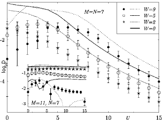
Figure 21: $\log{D}$ as a function of the interaction $U$ for $W=(0,)2,5,9$ for $M=N=7$ (for $M=11$, $N=7$ in the inset). For intermediate levels of interactions, a curve increase is observed. Specifically, for the sample and $W=9$, a minimum occurs at $\log{D}=-4.2$.

For a disorder equal to zero, the phase sensitivity is equal to zero for the half-filled case, $M=N=7$. The results show for the sample, an absence of Anderson localization for $U=0$. Moreover the sign of the phase sensitivity depends on the on-site disorder potentials and is random. This renders the averaging process difficult. Mean averages must be performed on $\Delta E$, and the fluctuations are in such a case much more significant than for systems with an even number of electrons. This is shown in Fig. 21. The averaged stiffness terms $\langle\log{D}\rangle$ respect Anderson localization for $U=0$ for both systems. For moderate values of the interactions and for the disorders $W=2,5,9$, an increase of $\log{D}$ is observed for the mean calculated averages and some various studied samples (except here for $W=2,5$ at half-filling). But in all cases, $\log{D}$ is smaller than that observed for an even number of electrons. Nevertheless $\log{D}$ can reach an order of magnitude ($D_{\rm max}/D(U=0)\sim 34$), at half-filling ($M=N=7$) and for $W=9$. For stronger interactions, the stiffness parameter decreases with $U$. At half-filling, the disorder increases the magnitude of the persistent current within the very strong interaction limits as what was observed for the case of even numbers of electrons. Finally, a perturbative approach is not possible as those theorems are applied uniquely for the case of even numbers of both sites and electrons.

- (1) M. Büttiker, Y. Imry and R. Landauer, Phys. Lett. A 96 A, 365 (1983).
- (2) L.P. Lévy, G. Dolan, J. Dunsmuir, and H. Bouchiat, Phys. Rev. Lett. 64, 2074 (1990).
- (3) V. Chandrasekhar, R.A. Webb, M.J. Brady, M.B. Ketchen, W.J. Gallagher, and A. Kleinsasser, Phys. Rev. Lett. 67, 3578 (1991).
- (4) D. Mailly, C. Chapellier, and A. Benoît, Phys. Rev. Lett. 70, 2020 (1993).
- (5) F. von Oppen and E.K. Riedel, Phys. Rev. Lett. 66, 84 (1991).
- (6) B.L. Altshuler, Y. Gefen and Y. Imry, Phys. Rev. Lett. 66, 88 (1991).
- (7) A. Schmid, Phys. Rev. Lett. 66, 80 (1991).
- (8) E.M.Q. Jariwala, P. Mohanty, M.B. Ketchen, and R.A. Webb, Phys. Rev. Lett. 86, 1594 (2001); W. Rabaud, L. Saminadayar, D. Mailly, K. Hasselbach, A. Benoît, and B. Etienne, Phys. Rev. Lett. 86, 3124 (2001).
- (9) D. Loss, Phys. Rev. Lett. 69, 343 (1992).
- (10) G. Montambaux, H. Bouchiat, D. Sigeti and R. Friesner, Phys. Rev. B 42, R7647 (1990).
- (11) U. Eckern and P. Schwab, J. of Low Temp. Physics 126, 1291 (2002) and references therein.
- (12) V. Ambegaokar and U. Eckern, Phys. Rev. Lett., 65, 381 (1990).
- (13) G. Bouzerar, D. Poilblanc, G. Montambaux, Phys. Rev. B 49, 8258 (1994).
- (14) H. Kato, D. Yoshioka, Phys. Rev. B 50, R4943 (1994).
- (15) R. Berkovits, Phys. Rev. B 48, 14381 (1993).
- (16) A. Cohen, K. Richter, and R. Berkovits, Phys. Rev. B 57, 6223 (1998).
- (17) M. Abraham, R. Berkovits, Phys. Rev. Lett. 70, 1509 (1993).
- (18) P. Schmitteckert, R.A. Jalabert, D. Weinmann and J.-L. Pichard, Phys. Rev. Lett. 81, 2308 (1998).
- (19) D.L. Shepelyansky, Phys. Rev. Lett. 73, 2607 (1994).
- (20) G. Benenti, X. Waintal and J.-L. Pichard, Phys. Rev. Lett. 83, 1826 (1999).
- (21) T. Giamarchi, B.S. Shastry, Phys. Rev. B 51,10915 (1995).
- (22) R.A. Römer and A. Punnoose, Phys. Rev. B 52, 14809 (1995).
- (23) H. Mori and M. Hamada, Phys. Rev. B 53, 4850 (1996).
- (24) E. Gambetti-Césare, D. Weinmann, R.A. Jalabert, P. Brune, EuroPhys. Lett. 60, 120 (2002).
- (25) Density-Matrix Renormalization – A New Numerical Method in Physics, ed. by I. Peschel, X. Wang, M. Kaulke, and K. Hallberg (Springer, Berlin, 1999).
- (26) S.R. White, Phys. Rev. Lett. 69, 2863 (1992).
- (27) E. Gambetti-Césare, ”Effet des Corrélations Électroniques et du Spin sur les Courants Permanents dans les Anneaux Unidimensionnels Désordonnés”, PhD thesis of the Louis Pasteur University, Strasbourg, http://tel.ccsd.cnrs.fr/documents/archives0/ 00/74/46/index_fr.html.
- (28) J. Hubbard, Proc. Roy. Soc. Ser. A, 240, 539, 1957; Proc. Roy. Soc. Ser. A, 243, 336 (1958); P.W. Anderson, Phys. Rev. 109, 5, 1492, (1958).
- (29) N. Byers and C.N. Yang, Phys. Rev. Lett., 7, 46 (1961).
- (30) W. Kohn, Phys. Rev. 133, A171 (1964).
- (31) P. Brune, A. Kampf, Europhys. Journal B, 18, 2, 241 (2001).
- (32) H. Bouchiat and G. Montambaux, J. Phys. France 50, 2695 (1989).
- (33) D. Weinmann, P. Schmitteckert, R.A. Jalabert, J.-L. Pichard, Eur. Phys. J. B, 19,139 (2001).
- (34) A. Auerbach, in Interacting Electrons and Quantum Magnetism, Springer, New York, 1994 and references therein.
- (35) E. Lieb et D. Mattis, Journal of Mathematical Physics 3, 4, (1962); E. H. Lieb et al., Ann. Phys. (N.Y.) 16, 407 (1961); E.H. Lieb, Phys. Rev. 125, 164 (1962).
- (36) E. H. Lieb,Proceedings of the conference Advances in Dynamical Systems and Quantum Physics , 1993, World Scientific, 173-193; Proceedings of ”The Hubbard model: its physics and mathematical physics”, New York: Plenum Press, 1995, 1-19; Proceeding of the XIth of the International Congress of Mathematical Physics, International Press, 1995, 392-412. Archived on cond-mat/9311033.
- (37) W. Marshall, Proc. R. Soc. London, Ser. A 232, 48 (1955).
- (38) H. Tasaki, Journal of Physics: Condensed Matter, 10, 4353-4378 (1998); H. Tasaki, Prog. Theo. Phys, 99, 489 (1998).
- (39) F. Selva and D. Weinmann, Eur. Phys. J. B, 18, 137 (2000).
- (40) A.J. Leggett, in Granular Nanoelectronics, edited by D.K. Ferry, J.R. Barker, and C. Jacobini, NATO ASI Ser. B251 (Plenum, New York, 1991).
- (41) C. A. Stafford, A. J. Millis, B. S. Shastry, Phys. Rev. B 43, 13660 (1991).
- (42) P.A. Lee and T.V. Ramakrishnan, Rev. Mod. Phys, 57, 287 (1985); B. Kramer and A. MacKinnon, Rep. Prog. Phys, 56, 1469 (1993).
- (43) M. Ramin, B. Reulet, H. Bouchiat, Phys. Rev. B, 51, R5582 (1995).
- (44) Y. Nagaoka, Phys. Rev., 147 (1), 392 (1966).
- (45) B. Simon, The statistical mechanics of lattice gases, livre 1, 130 (1993).
- (46) Z.Y. Weng, D.N. Sheng, C.S. Ting and Z.B. Su, Phys. Rev. Lett., 67, 3318 (1991); Z.Y. Weng, Phys. Rev. B, 50, 13837 (1994).
- (47) A. Müller-Groeling, H.A. Weidenmüller, C.H. Lewenkopf, Europhys. Lett. 22, 193 (1993); A. Müller-Groeling, H.A. Weidenmüller, Phys. Rev. B, 49, 4752 (1994).
- (48) P.J.H. Denteneer, R.T. Scalettar and N. Trivedi, Phys. Rev. Lett.87, 146401 (2001).
- (49) G. Bouzerar, D. Poilblanc, Phys. Rev. B 52, 10772 (1994).
- (50) N.F. Mott, Metal-Insulator Transitions, Taylor and Francis, London, 2nd. edition (1990).
- (51) E.H. Lieb, F.Y. Wu, Phys. Rev. Lett., 20, 1445 (1968); E.H. Lieb, F.Y. Wu, Physica A, 312, 1 (2003).
- (52) R.A. Jalabert, D. Weinmann, J-L. Pichard, Physica E, 9, 347 (2001).
- (53) S.V. Kravchenko, G.V. Kravchenko, J.E. Furneaux, V.M. Pudalov and M. D’Iorio, Phys. Rev. B, 50, 8039 (1994); S. V. Kravchenko, W. E. Mason, G. E. Bowker, J. E. Furneaux, V. M. Pudalov, and M. D’Iorio, Phys. Rev. B, 51, 7038-7045 (1995).
- (54) C. A. Stafford, A. J. Millis, Phys. Rev. B 48, 1409 (1993).