Proposed strategy to sort semiconducting nanotubes by radius and chirality

Abstract

We propose a strategy that uses a tunable laser and an alternating non-linear potential to sort a suspension of assorted semiconducting nanotubes. Since, a polarized exciton is a dipole, the excited nanotubes will experience a net force and may then diffuse towards an electrode. The calculated exciton binding energy suddenly drops to zero and the force on the nanotube increases dramatically when the exciton disassociates as the nanotube moves towards the electrode. The quantum adiabatic theorem shows that excitons will be polarized for potential frequencies typical for experiments $\approx 10$ MHz.

The unexpected discovery of another state of carbon in single walled carbon nanotubesSaito et al. (1998) (SWNTs) has attracted a great deal of theoretical and technological interest. SWNTs can be semiconducting or metallicSaito et al. (1998) depending on their chirality and diameter, and may be combined to create exotic devices. Typically an assortment of SWNTs bound by strong van-der-waals forces are created, thus individual SWNTs are hard to manipulate. Recently, SWNT ropes were seperated in water (containing a surfactant) by sound waves and centrifugationO’Connell et al. (1991). The resulting suspension contained SWNTs with an average diameter and length of $0.7$ nm and $130$ nm respectively. Metallic and semiconducting SWNTs have subsequently been separatedKrupke et al. (2003) by alternating current (AC) dielectrophoresisPohl (1978). This paper proposes theoretically a strategy for sorting the remaining semiconducting SWNTs according to radius and chirality.

An electrode defines an alternating exponentially decaying potential in the suspension, and laser pulses excite electron-hole ($e-h$) pairs. Since the band gap conveniently scales with the inverse of the diameter (where a diameter between $0.6$ to $1.6$ nm corresponds to $0.4-1.0$ eV) the laser frequency can be tuned to select some nanotubesIchida et al. (2004). The external potential frequency is “slow” so that the $e-h$ hole pairs are polarized adiabatically, but also “fast” enough to prevent the build up of a surface charge and its associated electrophoretic force. The $e-h$ pairs are expected to initially screen the external potential Gulbinas et al. (2004) which will recover as the exciton density decays. The remaining excitons, as in the p-n junction of a nanotube solar cellFreitag et al. (2003), shall disassociate and migrate to opposite ends. The excitonic dipole experiences a net time average force and the host nanotube may then diffuse towards the electrode, whereas the inert nanotubes will remain in place; this is the essence of the separation strategy which can be classified as light-induced AC dielectrophoresis. The exciton is considered quantum mechanically to calculate the force on a bare nanotube, and its dipole moment to estimate the interaction with the medium.

The time dependent Hamiltonian for an electron and hole on the surface of a nanotube with positions $r_{1}$ and $r_{2}$ with masses $m_{1}$ and $m_{2}$ has the form

$$H=p_{r_{1}}^{2}/2m_{1}+p_{r_{1}}^{2}/2m_{1}+V_{C}\left(r_{1},r_{2}\right)+V_{ext}$$ (1)

where the external potential $V_{ext}=e(t/T)(V_{0}e^{-kz_{1}}-V_{0}e^{-kz_{2}})$, $V_{c}$ is the attractive Coulomb potential, and $V_{0}$ and $k$ are constants determined by the gate bias and geometry. Within one cycle the external potential increases adiabatically from zero to its full value for $0<t<T$ during the polarization time $T$. The adiabatic regime implies, that instantaneous eigenstates can be calculated using an effective time independent Hamiltonian.

In an effort to illustrate the physical trends of the system we have calculated the adiabatic exciton ground state using a simple Hartree model by assuming a separable wavefuction $\Phi(r_{1},r_{2})=\Phi(r_{1})\Phi(r_{2})$ and neglecting bandstructure effectsKostov et al. (2002); Pedersen (2003). Since the nanotube length is much greater than its diameterPedersen et al. (2000); Ogawa and Takagahara (1991) the wavefunction in the radial direction can be assumed to be dominated by directions strong confinement. The radial kinetic energy is assumed to be much larger than the electron-hole interaction potential since the exciton radius will be much larger than the carbon bond length. Mathematically this suggests that we can assume that the electron and hole wavefunctions are separable in $z$ and $\theta$ coordinates, reducing this 2D problemJanssens et al. (2002) to a 1D problem. The ground state wavefunction for a nanotube with radius $r$ in the radial direction has the form $\Psi(\theta)=e^{-i\lambda\theta}{(2\pi)}^{-1/2}$ where the energy $\lambda=\hbar^{2}/(2mr^{2})$. The Hartree equations expressed in cylindrical polar coordinates are then,

$$\left[{p_{i}^{2}\over{2m_{i}}}+V{ij}+V_{ext}(z_{i})\right]\Psi\left(\theta_{i}\right)\Psi_{i}\left(\bf{z_{i}}\right)=E_{i}\Psi\left(\theta_{i}\right)\Psi\left(\bf{z_{i}}\right)$$

$$V{ij}\left(z_{i},\theta_{i}\right)=\int\limits_{0}^{\infty}dz_{j}\int\limits_{0}^{2\pi}d\theta_{j}\Psi(z_{j})^{2}{1\over{8\pi^{2}\epsilon}}{1\over{\sqrt{d}}}$$

$$i,j=e,h$$

$$j\neq i$$ (2)

where $V_{ij}$ is the electron-hole Coulomb potential, $d=r^{2}(2-\cos(\theta_{i}-\theta_{j}))+(z_{i}-z_{j})^{2}$, and $\epsilon$ is the dielectric constant. Multiplying by $e^{i\lambda\theta_{i}}{(2\pi)}^{-1/2}$ and integrating over $\theta$ coordinates we get,

$$\left[{-\hbar^{2}\over{2m}}{\partial\over{\partial^{2}z}}+V_{i}(z_{i})+V_{ext}\right]\Psi(z_{i})=\left[E_{i}-{\hbar^{2}\over{2mr^{2}}}\right]\Psi(z_{i})$$ (3)

and $V_{i}(z_{i})=\int V_{eff}(z_{i}-z_{j})\Psi(z_{j})dz_{j}$ where an effective potential $V_{eff}$ is defined as,

$$V_{eff}(z_{i}-z_{j})={1\over{4\pi^{2}}}\int{1\over{4\pi\epsilon}}{1\over{\sqrt{d}}}d\theta_{i}d\theta_{j}$$ (4)

Since the effective potential has no analytic form we follow previous worksJan et al. (1994); Pedersen et al. (2000) and approximate the effective potential to a simple form $V_{eff}\approx U_{eff}=1/(4\pi\epsilon)[\sigma^{2}-(z_{i}-z_{j})^{2}]^{-1/2}$, where $\sigma$ is a parameter adjusted to make $U_{eff}$ resemble the numerically integrated average potential $V_{eff}$. The Hartree equations are then discretized and solved self consistently.

We assume throughout that the torque generated by the external potential has aligned the nanotube. We have calculated the exciton binding energy, the dipole moment $p=e|\langle\Psi|z|\Psi\rangle|$ and the instantaneous acceleration $a$ experienced by a nanotube with length $L$ whose left edge is a distance $d$ from the origin. The acceleration $a$ is related to the electron $\rho_{e}$ and hole $\rho_{h}$ charge densities,

$$a(z,L)={{1}\over{\mu L}}\int_{d}^{d+L}kV_{ext}(z)\left[\rho_{e}(z)-\rho_{h}(z)\right]dz$$ (5)

where the nanotubes mass $m_{t}=\mu L$ where $\mu$ is a constant depending on the number of atoms per unit cell.

We consider a typical semiconducting SWNT the $(12,0)$ with diameter $0.994$ nm and a unit cell of length $0.85$ nmLehtinen et al. (1994) which contains $96$ carbon atoms. We have set $m_{e}=m_{h}=0.08m_{0}$ (unless stated otherwise), a typical value for a small diameter semiconducting SWNTPedersen et al. (2000), $\epsilon=3.3$Pedersen et al. (2000), and $\sigma=0.45$ nm. The results are presented for an external potential characterized by $k=0.001$ in atomic units, and $V_{0}=2.0$ V.

Fig1 shows the binding energy (BE) as a function of $d$ and $t$ for $L=20-50$ nm. Since the electron-hole attraction is strong in nanotubes which are approximate 1D systemSpataru et al. (2004), the BE is relatively large $\approx 0.6$ eV when the nanotube is far from the electrode. The BE drops suddenly to zero at a position dependent critical time $t_{c}(d)$ indicating a structural transition in the excitons wavefunction. The exciton BE depends on the balance between the attractive Coulomb interaction and the potential drop along the nanotube. The exciton is clearly harder to polarize as the nanotube length decreases since the potential drop along the nanotube is less and the electron and hole are restricted to within a smaller volume. The forces involved: the Coulomb attraction and the external potential are all non-linear, which explains the non-linear relation between $d_{c}(t)$ with the length $L$.

Fig 2 shows the structural transition of the excitons wavefunction for $t/T=1.0$ as a nanotube with length $L=30$ nm is moved towards the gate. The balance between the polarizing effect of the external potential and the Coulomb attraction between the electron and hole determines the exciton’s structure. The exciton is strongly bound when the nanotube is far from the gate and resides at the the end which is furtherest away from the gate. As the nanotube is moved closer, the electron charge density piles towards the end closer to the electrode and drags the hole along. Finally, around $d_{c}$ the electron and hole are located at opposite ends of the nanotube and the exciton has disassociated.

We have assumed so far that the exciton has been polarized adiabatically. The adiabatic characteristic time $T_{a}$ can be determined from the adiabatic theorem which requires an estimate of the exciton energy spectra. Specifically, we need to calculate the two lowest exciton states $|\Phi_{\alpha}\rangle$ and $|\Phi_{\beta}\rangle$ with energies $E_{\alpha}$ and $E_{\beta}$. Typically, the conduction and valence band of a semiconducting nanotube contains degenerate bands. We calculate the ground state by assuming that $m_{e}=m_{h}=0.08m_{0}$ and for the first excited state the electron has occupied the light band with $m_{e}=0.05m_{0}$Zhao et al. (2004). The adiabatic theorem imposesMartins et al. (2004),

$$T\gg T_{a}=\hbar\Gamma{max}/g^{2}_{min}$$ (6)

where $g_{min}=min_{0<t<T}\left[E_{\alpha}(t)-E_{\beta}(t)\right]$ and $\Gamma_{max}=max_{0<t<T}|\langle\Phi_{\alpha}|eV_{0}(e^{-kz_{1}}-e^{kz_{2}})|\phi_{\beta}\rangle|$. Fig 3 shows the time dependence of the exciton binding energies of these states for a nanotube with length $L=50$ nm and $d=25$ nm. Evidently, after a critical time the external potential is able to disassociate the exciton and the binding energy drops to zero. The higher energy state $\beta$ with more kinetic energy, is marginally more easier to disassociate. For these parameters $g_{min}=1.37$ meV and $T_{a}=4.9$ ps. Since the bands in the conduction and/or valence band(s) are often separated by an energy gap of the order of $0.1$ eVReich et al. (2002), $T_{a}=4.9$ ps represents a deliberately high estimate. The external potential in experiments usually has a frequency $10$ MHz corresponding to $T\approx 10^{-8}$ s thus excitons will be polarized, though thermal effects will have to included to determine the charge distribution.

Typically the dielectric constant ($\epsilon<5$) for semiconducting nanotubes is small compared to that of water $\epsilon_{w}=80.0$. These values when inserted into the expression for the dielectrophoretic force on a sphere indicatesKrupke et al. (2003) negative dielectrophoresis i.e. no attraction to the electrode. The metal nanotubes in contrast have a large dielectric constantBenedict et al. (1995) (perhaps infinite) in comparison to that of water and subsequently experience positive dielectrophoresis and are strongly attracted to the electrodeKrupke et al. (2003). The dielectric constant of an excited nanotube can be estimated by considering the contribution to the dipole momentBianchetti et al. (2002) from the excitonWarburton et al. (2002) as shown in Fig 4. The exciton dipole moment even for modest electric fields is much bigger than that of a water molecule ($6.19\times 10^{-30}$ Cm) since an exciton is a delocalized and weakly bound entity in comparison to a molecule. The dipole moment increases dramatically when the exciton disassociates, so the polarizabilty is greatest during this transition. The dielectric constant of the nanotube cannot be determined using the Clausius-Mossoti relationOrtuno and Chicon (1989) since this is only valid for a weakly polarizable material. A large dielectric constant is indicated here however, since a substantial cancelation of the applied field by the mobile charges is expected, so an excited nanotube is expected undergo positive dielectrophoresis. We note that highly polarizable materials have enormous dielectric constants: living organisms such as yeastProdan et al. (2000) ($\epsilon>10^{5}$) contain mobile charges which can screen the applied field, and a perovskite related oxideHomes et al. (2001) which is suspected to contain responsive dipoles also has large dielectric constant. We expect excited nanotubes to have a similarly large dielectric constant.

Fig 5 shows the instantaneous acceleration $a$ as a function $d$ and $t$ for nanotubes with lengths $L=20-50$ nm. Comparing with Fig 1 $a$ increases by several orders of magnitude when the exciton disassociates and the electron and hole reside at opposite ends of the nanotube. The motion of a nanotube will be hindered by collisions with the molecules of the liquid and will be strongly dependent on the nanotube length. The dependence of the nanotube motion with length, can be the basis of its seperation according to length by a thermal ratchet mechanismvan Oudenaarden and Boxer (1999). The result indicate that exciton disassociation can be achieved using modest electric field gradients. The field may have to further increased however to overcome the random Brownian motion of the nanotube.

We have suggested a method to sort semiconducting nanotubes using dielectrophoresisKrupke et al. (2003) and spectroscopy techniquesOstogic et al. (2005). Since both of these methods have been separately applied to nanotubes, it should be relatively straight forward to combine them within a single experiment. The experiments can be accurately modeled by including the exciton creation and annihilation ratesBunning et al. (2005) and the interaction with the liquid by molecular dynamics simulationsEnglish and MacElroy (2003). Recently, solar cellsMcDonald et al. (2005) have been made from polymers-quantum dots composites. The quantum dots formed in solution can be separated according to their band-gap using light induced dielectrophoresis to optimize the solar cell. We anticipate that future devices can be self assembled by carefully fabricating electrodes and to define electric field linesHunt et al. (2004) that will guide nano-ojects to the required place. We hope this paper will stimulate future experimental and theoretical work.

Figure Captions

Figure 1

The binding energy as a function of $d$ and $t/T$ for $L=50$ nm (top), $L=35$ nm (middle) and $L=20$ nm (bottom). The lines are shown for $t/T=0.1-1.0$ in steps of $0.1$, and some lines are labelled.

Figure 2

The electron (top) and hole (bottom) charge densities for a nanotube with length $L=30$ nm, for $d=39.15$ nm (full lines), $d=39.05$ nm (dotted lines), and $d=37.65$ nm (dashed lines). The lines are shown for $t/T=1$.

Figure 3

The binding energies as a function of $t$ for the ground state (dotted line) and first excited state (full lines). Here $L=50$ nm, $d=25$ nm, $m_{e}=m_{h}=0.08m_{0}$ for the ground state, and $m_{e}=0.05m_{0}$ and $m_{h}=0.08m_{0}$ for the excited state.

Figure 4

The dipole moment of a nanotube with length $L=50$ nm as a function of an applied linear electric field. The polarizability is the gradient.

Figure 5

The log of the instantaneous acceleration as a function of $d$ and $t/T$ for $L=50$ nm (top), $L=35$ nm (middle) and $L=20$ nm (bottom). The lines are shown for $t/T=0.1=1.0$ in steps of $0.1$, and some lines are labelled.

Figure 1: V. Narayan PRL

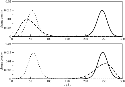
Figure 2: V. Narayan PRL

Figure 3: V. Narayan PRL

Figure 4: V. Narayan PRL

Figure 5: V. Narayan PRL

References

- Saito et al. (1998) R. Saito, G. Dresselhaus, and M. S. Dresselhaus, Physical properties of carbon nanotubes (Imperial College Press, 1998).
- O’Connell et al. (1991) M. J. O’Connell, S. M. Bachilo, C. B. Huffman, V. C. Moore, M. S. Strano, E. H. Haroz, K. L. R. P. J. Boul, W. H. Noon, C. Kittrell, J. Ma, et al., Science 354, 56 (1991).
- Krupke et al. (2003) R. Krupke, F. Hennrich, H. v. Löhneysen, and M. M. Kappes, Science 301, 344 (2003).
- Pohl (1978) H. A. Pohl, Dielectrophoresis (Cambridge University Press, 1978).
- Ichida et al. (2004) M. Ichida, Y. Hamanaka, H. Katura, Y. Achiba, and A. Nakamura, J. Phys. Soc. Jap. 73, 3479 (2004).
- Gulbinas et al. (2004) V. Gulbinas, Y. Zaushitsyn, H. Bässler, A. Yartsev, and V. Sundtröm, Phys. Rev. B 70, 035215 (2004).
- Freitag et al. (2003) M. Freitag, Y. Martin, J. A. Misewich, R. Martel, and P. Avouris, Nano Letters 3, 1067 (2003).
- Kostov et al. (2002) M. K. Kostov, M. W. Cole, and G. D. Mahan, Phys. Rev. B 66, 075407 (2002).
- Pedersen (2003) T. G. Pedersen, Phys. Rev. B 67, 073401 (2003).
- Pedersen et al. (2000) T. G. Pedersen, P. M. Johannsen, and H. C. Pedersen, Phys. Rev. B 61, 10504 (2000).
- Ogawa and Takagahara (1991) T. Ogawa and T. Takagahara, Phys. Rev. B 44, 8138 (1991).
- Janssens et al. (2002) K. L. Janssens, B. Partoens, and F. M. Peeters, Phys. Rev. B 66, 075314 (2002).
- Jan et al. (1994) J. F. Jan, Y. C. Lee, and D. S. Chuu, Phys. Rev. B 50, 14647 (1994).
- Lehtinen et al. (1994) P. O. Lehtinen, A. S. Foster, A. Ayuela, T. T. Vehvilainen, and R. M. Nieminen, Phys. Rev. B 50, 14647 (1994).
- Spataru et al. (2004) C. D. Spataru, S. Ismail-Beigi, L. X. Benedict, and S. G. Louie, Phys. Rev. Lett. 92, 077402 (2004).
- Zhao et al. (2004) G. L. Zhao, D. Bagayoko, and L. Yang, Phys. Rev. B 69, 245416 (2004).
- Martins et al. (2004) A. S. Martins, R. B. Capaz, and B. Koiller, Phys. Rev. B 69, 085320 (2004).
- Reich et al. (2002) S. Reich, C. Thomson, and P. Ordejon, Phys. Rev. B 65, 155411 (2002).
- Benedict et al. (1995) L. X. Benedict, S. G. Louie, and M. Cohen, Phys. Rev. B 52, 8541 (1995).
- Bianchetti et al. (2002) M. Bianchetti, P. F. Buonsante, F. Ginelli, H. E. Roman, R. A. Broglia, and F. Alasia, Phys. Rep. 459, 513 (2002).
- Warburton et al. (2002) R. J. Warburton, S. Schulhauser, D. Haft, C. Schäflein, J. M. Garcia, W. Schoenfeld, and P. M. Petroff, Phys. Rev. B 65, 113303 (2002).
- Ortuno and Chicon (1989) M. Ortuno and R. Chicon, Am. J. Phys. 57, 818 (1989).
- Prodan et al. (2000) C. Prodan, J. R. Claycomb, E. Prodan, and J. H. Miller, Physica C 341, 2693 (2000).
- Homes et al. (2001) C. C. Homes, T. Vogt, S. M. Shapiro, S. Wakimoto, and A. P. Ramirez, Science 293, 673 (2001).
- van Oudenaarden and Boxer (1999) A. van Oudenaarden and S. G. Boxer, Science 285, 1046 (1999).
- Ostogic et al. (2005) G. N. Ostogic, S. Zaric, J. Kono, V. C. Moore, R. H. Hauge, and R. E. Smalley, Phys. Rev. Lett. 94, 097401 (2005).
- Bunning et al. (2005) J. C. Bunning, K. J. Donovan, K. Scott, and M. Somerton, Phys. Rev. B 71, 085412 (2005).
- English and MacElroy (2003) N. J. English and J. M. D. MacElroy, J. Chem. Phys. 119, 11806 (2003).
- McDonald et al. (2005) S. A. McDonald, G. Konstrantatos, S. Zhang, P. W. Cyr, E. J. D. Klem, L. Levina, and E. H. Sargent, Nature Mat. 4, 138 (2005).
- Hunt et al. (2004) T. P. Hunt, H. Lee, and R. M. Westervelt, Appl. Phys. Lett. 85, 8421 (2004).