Band structure and magnetotransport of a two-dimensional electron gas in the presence of spin-orbit interaction

Abstract

The band structure and magnetotransport of a two-dimensional electron gas (2DEG), in the presence of the Rashba (RSOI) and Dresselhaus (DSOI) terms of the spin-orbit interaction and of a perpendicular magnetic field, is investigated. Exact and approximate analytical expressions for the band structure are obtained and used to calculate the density of states (DOS) and the longitudinal magnetoresitivity assuming a Gaussian type of level broadening. The interplay between the Zeeman coupling and the two terms of the SOI is discussed. If the strengths $\alpha$ and $\beta$, of the RSOI and DSOI, respectively, are equal and the $g$ factor vanishes, the two spin states are degenerate and a shifted Landau-level structure appears. With the increase of the difference $\alpha-\beta$, a novel beating pattern of the DOS and of the Shubnikov-de Haas (SdH) oscillations appears distinctly different from that occurring when one of these strengths vanishes.

I introduction

The spin-orbit interaction (SOI) in semiconductor nanostructures has attracted extensive attention in the past years mostly due to its potential applications in manipulating electron spins in electronic devices and its ample physical characteristics hidden and unexplored previously. The SOI is a relativistic coupling between the spin and momentum of an electron under an external electric field. wink This external electric field can be the slope of the band structure or the averaged crystal field due to an asymmetry of the bulk semiconductor crystal. The former results in the Rashba SOI (RSOI) bych and the later in the Dresselhaus SOI (DSOI). dres In semiconductor heterostructures an additional DSOI arises from the asymmetry of the material growth at the interfaces that is different from that due to the crystal asymmetry in bulk materials. dyak ; verv ; ross

The RSOI is rotationally symmetric in a 2DEG and normally dominates in 2DEG’s of many narrow-gap semiconductors such as InGaAs/AlGaAs. wang2 This has been confirmed in experiments luo ; koga . Recent experiments, however, show that the DSOI makes an important contribution to the SOI and can be dominant in 2DEG’s of materials shuch as InSb/InAlSb. gani ; here In a system without magnetic field, it has been shown that the DSOI introduces a strong anisotropy to the electronic energy band and the electron transport. gani ; schl1 An interesting phenomenon in this case is that $k$-independent eigenspinors appear when the strengths $\alpha$ and $\beta$, of the RSOI and DSOI, respectively, are equal. schl1

It is well known that under a perpendicular magnetic field the Hamiltonian can be solved exactly if only one of the RSOI or the DSOI terms exists. Two branches of energy levels with unequal separations between adjacent levels develop and lead to a beating pattern of the SdH oscillations observed in moderate magnetic fields. luo ; koga ; nitt ; wink ; wang By measuring the position of the nodes of the beating pattern, one can estimate the strength $\alpha$ or $\beta$ of the SOI. The situation is much less clear when both terms of the SOI are present as the number of pertinent studies is limited gani . In particular, we are not aware of any treatment of the band structure and SdH oscillations of a 2DEG under a perpendicular magnetic field when both terms of the SOI are present. We provide one in this paper and organize it as follows. In Sec. II we provide exact and approximate results for the energy spectrum and the DOS. In Sec. III we present analytical and numerical results for the transport coefficients, and in Sec. V concluding remarks.

II Eigenvectors, eigenvalues, and density of states

We consider a 2DEG in the $(x-y)$ plane and a magnetic field along the $z$ direction. In the Landau gauge $\vec{A}=(0,Bx,0)$ the one-electron Hamiltonian $H=H_{0}+H_{\alpha}+H_{\beta}$ including the SOI Rashba term, $H_{\alpha}$, and the Dresselhaus SOI term, $H_{\beta}$, reads bych ; ross

$$H = \frac{(\hat{{\bf p}}+e{\bf A})^{2}}{2m^{\ast}}+\frac{1}{2}g_{s}\mu_{B}B\sigma_{z},+H_{\alpha}+H_{\beta}$$ (1)

$$H_{\alpha} = \frac{\alpha}{\hbar}\sigma_{x}(\hat{p}_{y}+eA_{y})-\frac{\alpha}{\hbar}\sigma_{y}(\hat{p}_{x}+eA_{x}),$$

$$H_{\beta} = \frac{\beta}{\hbar}\sigma_{x}(\hat{p}_{x}+eA_{x})-\frac{\beta}{\hbar}\sigma_{y}(\hat{p}_{y}+eA_{y}),$$

where $\hat{\bf p}=(\hat{p}_{x},\hat{p}_{y})$ is the momentum operator of the electrons, $m^{\ast}$ their effective mass, $g_{s}$ the Zeeman factor, $\mu_{B}$ the Bohr magneton, ${\bf\sigma}=(\sigma_{x},\sigma_{y},\sigma_{z})$ the Pauli spin matrix, and $\alpha$, $\beta$ the strengths of the Rashba and Dresselhaus terms, respectively.

In the absence of SOI the eigenstates of the Hamiltonian are the Landau states $|n,\sigma\rangle$, $n=0,1,2,\cdots$, with energy $\varepsilon_{n}^{\sigma}=(n+1/2)\hbar\omega_{c}+\sigma g_{s}\mu_{B}B/2$, and wave function $\langle{\bf r}|n,\sigma\rangle=e^{ik_{y}y}\phi_{n}(x+x_{c})|\sigma\rangle/\sqrt{L_{y}}$. $L_{y}$ is the length of the system along the $y$ direction, $\phi_{n}(x+x_{c})=e^{-(x+x_{c})^{2}/2l_{c}^{2}}H_{n}((x+x_{c})/l_{c})/\sqrt{\sqrt{\pi}2^{n}n!l_{c}}$ the harmonic oscillator function, $\omega_{c}=eB/m^{\ast}$ the cyclotron frequency, $l_{c}=(\hbar/m^{\ast}\omega_{c})^{1/2}$ the radius of the cyclotron orbit centered at $-x_{c}=-l_{c}^{2}k_{x}$, $n=0,1,2,\cdots$ the Landau-level index, and $|\sigma\rangle=|\pm\rangle$ the electron spin written as the row vector $|+\rangle=(0,1)$ if the spin points up and as $|+\rangle=(1,0)$ if it points down.

Generally, the SOI groups the Landau states into two groups $|n,\sigma_{n}\rangle$ and $|n,-\sigma_{n}\rangle$ with $\sigma_{n}=(-1)^{n}$ and couples the states with each other in each group. Assuming eigenstates in the form of $\Psi=\sum_{n}C_{n}^{\sigma}|n,\sigma\rangle$, the secular equation $H\Psi=E\Psi$ leads to the system of equations

$$\sqrt{n}\epsilon_{\alpha}C_{n-1}^{+}+(\varepsilon_{n}^{-}-E)C_{n}^{-}-i\sqrt{n+1}\epsilon_{\beta}C_{n+1}^{+} = 0$$ (2)

$$i\sqrt{n+1}\epsilon_{\beta}C_{n}^{-}+(\varepsilon_{n+1}^{+}-E)C_{n+1}^{+}+\sqrt{n+2}\epsilon_{\alpha}C_{n+2}^{-} = 0,$$

with $n$ odd for the group $|n,\sigma_{n}\rangle$ and even for the group $|n,-\sigma_{n}\rangle$. Here $\epsilon_{\alpha}=\sqrt{2}\alpha/l_{c}$ and $\epsilon_{\beta}=\sqrt{2}\beta/l_{c}$. This means that the Hamiltonian matrix in the Landau space reduces to two independent, infinitely dimensional matrices. The matrix corresponding to the group $|n,\sigma_{n}\rangle$ reads

$$\left[\begin{array}[]{ccccccc}\varepsilon_{0}^{+}&\epsilon_{\alpha}&0&0&0&0&\cdots\\ \epsilon_{\alpha}&\varepsilon_{1}^{-}&-i\sqrt{2}\epsilon_{\beta}&0&0&0&\cdots\\ 0&i\sqrt{2}\epsilon_{\beta}&\varepsilon_{2}^{+}&\sqrt{3}\epsilon_{\alpha}&0&0&\cdots\\ 0&0&\sqrt{3}\epsilon_{\alpha}&\varepsilon_{3}^{-}&-i2\epsilon_{\beta}&0&\cdots\\ 0&0&0&i2\epsilon_{\beta}&\varepsilon_{4}^{+}&\sqrt{5}\epsilon_{\alpha}&\cdots\\ \cdots&\cdots&\cdots&\cdots&\cdots&\cdots&\cdots\end{array}\right]$$ (3)

and the one corresponding to the group $|n,-\sigma_{n}\rangle$

$$\left[\begin{array}[]{ccccccc}\varepsilon_{0}^{-}&-i\epsilon_{\beta}&0&0&0&0&\cdots\\ i\epsilon_{\beta}&\varepsilon_{1}^{+}&\sqrt{2}\epsilon_{\alpha}&0&0&0&\cdots\\ 0&\sqrt{2}\epsilon_{\alpha}&\varepsilon_{2}^{-}&-i\sqrt{3}\epsilon_{\beta}&0&0&\cdots\\ 0&0&i\sqrt{3}\epsilon_{\beta}&\varepsilon_{3}^{+}&2\epsilon_{\alpha}&0&\cdots\\ 0&0&0&2\epsilon_{\alpha}&\varepsilon_{4}^{-}&-i\sqrt{5}\epsilon_{\beta}&\cdots\\ \cdots&\cdots&\cdots&\cdots&\cdots&\cdots&\cdots\end{array}\right].$$ (4)

The energy spectrum of Eqs. (3) and (4) can be obtained numerically by truncating the matrix dimensions while including a sufficient number of Landau levels; the resulting energy spectrum will be referred to as the exact one in this paper. For $\alpha$ and $\beta$ varying independently, we study the spectrum in the ($\alpha$-$\beta$) plane and define an angle $\varphi$ at any point ($\alpha,\beta$) such that $\alpha=\gamma\cos\varphi$ and $\beta=\gamma\sin\varphi$ with $\gamma=(\alpha^{2}+\beta^{2})^{1/2}$. In Fig. 1 we show the spectrum (solid curves) as a function of the angle $\varphi$, in units of $\pi/2$, at various $\gamma$ values. The parameter $\alpha_{0}$ is equal to $10^{-11}$eVm. We consider only positive $\alpha$ and $\beta$ so that $0<\varphi<\pi/2$. Results for negative $\alpha$ or $\beta$ can be obtained by symmetry. The results for $g_{s}=0$ and $g_{s}=5$ shown present the effect of the Zeeman term. The value of $g_{s}$ varies from sample to sample in the literature but we use $g_{s}=5$ since a recent experiment demonstrated a $g_{s}$ range from 2 to 5 in gate-controlled InGaAs/InAlAs quantum wells. nit2 The SOI splits the Landau levels in two branches, referred to as the $+$ and $-$ branches, which cross each other when $\varphi$ is varied. The two spin branches in each Landau level are degenerate for $\alpha=\beta$ or $\varphi=\pi/4$ if the Zeeman term is absent; then energy-branch crossing shifts with increasing $g_{s}$. This energy degeneracy can occur for several values of $\varphi$ as shown by the upper curves in the plots with $\gamma=2\alpha_{0}$.

A better insight into the problem is obtained by an analytic energy spectrum. This can facilitate the study of other properties, e.g., the transport properties of this system. It is well known wang that the Hamiltonian (II) has an exact solution if $\alpha$ or $\beta$ vanishes. Here we will show that an exact result is obtained also for $\alpha=\beta$, if we neglect the Zeeman term, and approximate perturbative results follow for $\alpha/\beta\ll$ or $\gg 1$ and $\alpha\approx\beta$.

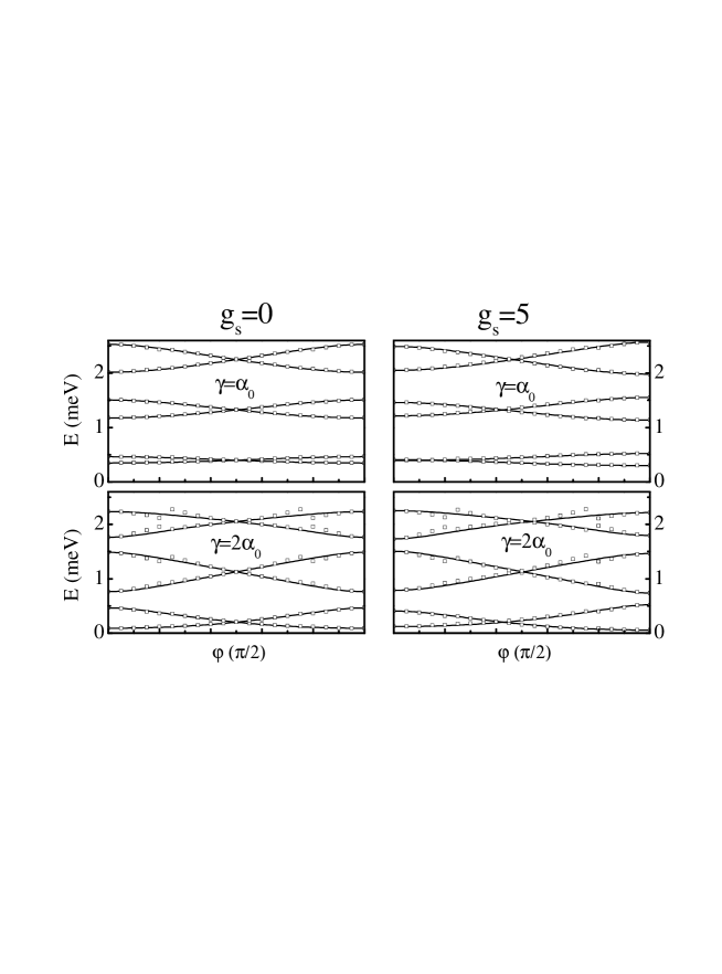
Figure 1: Energy spectrum of a 2DEG vs the angle $\varphi$ ($\tan\varphi=\alpha/\beta$) for two values of $\gamma=(\alpha^{2}+\beta^{2})^{1/2}$ in a perpendicular magnetic field $B=0.4$ T. The solid curves denote the numerical result, obtained by diagonalizing the Hamiltonian matrices (3) and (4), and the empty squares the approximate analytical result described by Eq. (9) for $\tan\varphi<1/3$, its $\beta\gg\alpha$ counterpart for $\tan\varphi>3$ , and by Eq. (16) for $1/3<\tan\varphi<3$. On the left panels the Zeeman term is neglected, on the right ones it is not ($g_{s}=5$). The effective electron mass used is $m^{\ast}=0.05m_{0}$.

II.1 Highly unequal strenths: $\alpha<<\beta$ or $\beta<<\alpha$

For $\beta=0$ the Hamiltonian $H_{0}+H_{\alpha}$ in the Landau space, cf. Eqs.(3) and (4), reduces to $2\times 2$ matrices with exact eigenvalues bych ; wang ; shen

$${\cal E}_{n}^{\sigma}=\hbar\omega_{c}(n+\sigma\sqrt{(1-g)^{2}+8nk^{2}_{\alpha}l^{2}_{c}}/2)$$ (5)

and eigenfunction

$$\Psi^{\sigma}_{n}=\frac{e^{ik_{y}y}}{\sqrt{L_{y}}}\left(\begin{array}[]{c}\phi_{n-1}(x+x_{c})\sin\theta^{\sigma}_{n}\\ \phi_{n}(x+x_{c})\cos\theta^{\sigma}_{n}\\ \end{array}\right).$$ (6)

Here $n=0,1,2,\cdots$ for $\sigma=1$ and $n=1,2,3,\cdots$ for $\sigma=-1$, $g=g_{s}m^{\ast}/m_{0}$ with $m_{0}$ the free-electron mass, $k_{\alpha}=\alpha m^{\ast}/\hbar^{2}$, $\theta^{-}_{n}=\theta^{+}_{n}-\pi/2$, and

$$\tan\theta^{+}_{n}=\frac{2\sqrt{2n}k_{\alpha}l_{c}}{1-g+\sqrt{(1-g)^{2}+8nk^{2}_{\alpha}l_{c}^{2}}}.$$ (7)

For $\beta<<\alpha$, we can treat $H_{\beta}$ as a perturbation of $H_{0}+H_{\alpha}$. Neglecting the cross terms $\propto\alpha\beta$, the matrix elements of $H_{\beta}$ are

$$\langle\Psi^{\sigma}_{m}|H_{\beta}|\Psi^{\sigma^{\prime}}_{n}\rangle=i(\sigma^{\prime}-\sigma)\sqrt{(m+\sigma)}(\epsilon_{\beta}/2)\delta_{m,n-2\sigma}.$$ (8)

Then the total Hamiltonian is a matrix composed of diagonal elements $\varepsilon^{-}_{1}$ and a series of $2\times 2$ diagonal blocks. The eigenvalues are

$$E_{t}^{\sigma}=({\cal E}^{-}_{t+1}+{\cal E}^{+}_{t-1})/2+(\sigma/2)\sqrt{({\cal E}^{-}_{t+1}-{\cal E}^{+}_{t-1})^{2}+4t\epsilon_{\beta}^{2}};$$ (9)

the corresponding wave functions read

$$f^{\sigma}_{t}=-i\Psi^{+}_{t-1}\sin\gamma^{\sigma}_{t}+\Psi^{-}_{t+1}\cos\gamma^{\sigma}_{t},$$ (10)

with $\tan\gamma^{\sigma}_{t}=(2\sqrt{t}\epsilon_{\beta})/[\sqrt{({\cal E}^{-}_{t+1}-{\cal E}^{+}_{t-1})^{2}+4t\epsilon_{\beta}^{2}}+\sigma({\cal E}^{-}_{t+1}-{\cal E}^{+}_{t-1})]$ and $t=1,2,3,\cdots$ for $\sigma=1$ or $t=0,1,2,\cdots$ for $\sigma=-1$.

The results corresponding to $\beta\gg\alpha$ can be obtained in the same way. The energy spectrum is still given by Eqs.(5) and (9) with $\alpha$ and $\beta$ interchanged and $(1-g)$ replaced by $(1+g)$. The wave functions are given by Eq. (6), with $\sin\theta^{\sigma}_{n}$ replaced by $-i\sin\theta^{\sigma}_{n}$, and by Eq. (10) with $-i\sin\gamma^{\sigma}_{n}$ replaced by $\sin\gamma^{\sigma}_{n}$. Equations (9) and (10) and their $\beta\gg\alpha$ counterpart will be used as an analytical approximation for $|\beta-\alpha|/(\alpha+\beta)>0.5$ or $\tan\varphi>3$ and $1/3<\tan\varphi$.

II.2 Equal ($\alpha=\beta$) or approximately equal ($\alpha\approx\beta$) strengths

For $\alpha=\beta$ the Hamiltonian $H=H_{0}+H_{\alpha}+H_{\beta}$ without the Zeeman term can be diagonalized by a unitary transformation $U^{\dagger}HU$ with

$$U=\left[\begin{array}[]{cc}(1+i)/2&-(1+i)/2\\ 1/\sqrt{2}&1/\sqrt{2}\end{array}\right].$$ (11)

The nonzero elements of the diagonalized Hamiltonian read

$$H_{\sigma,\sigma}=(\hat{p}_{x}+\sigma\sqrt{2}\hbar k_{s})^{2}/2m^{\ast}+(\hat{p}_{y}+\sigma\sqrt{2}\hbar k_{s}+eBx)^{2}/2m^{\ast}-2\hbar^{2}k_{s}^{2}/m^{\ast}$$ (12)

with $k_{s}=am^{\ast}/2\hbar^{2}$ and $a=(\alpha+\beta)/2$. This Hamiltonian is very close to that of a displaced harmonic oscillator and we attempt solutions in the form $\Psi^{\sigma}(x,y)=e^{ik_{y}y}e^{-i\sigma\sqrt{2}k_{s}x}\phi(x)$ for the spin branch $\sigma$. The wave function of this Hamiltonian, in the Landau gauge, is then obtained as

$$\Psi^{\sigma}_{n}=\frac{e^{ik_{y}y}}{\sqrt{L_{y}}}e^{-i\sigma\sqrt{2}k_{s}x}\phi_{n}(x+x_{c}+\sigma x_{s})\left(\begin{array}[]{c}\sigma(1+i)/2\\ 1/\sqrt{2}\end{array}\right)$$ (13)

with $x_{c}=l^{2}_{c}k_{y}$, $x_{s}=\sqrt{2}l^{2}_{c}k_{s}$ and eigenvalue

$${\cal E}^{\sigma}_{n}=(n+1/2)\hbar\omega_{c}-2\hbar^{2}k_{s}^{2}/m^{\ast}.$$ (14)

For $\alpha\neq\beta$ the Hamiltonian given by Eq. (II) after the unitary transformation has diagonal and nondiagonal elements. The diagonal ones are given by Eq. (12) and the nondiagonal ones by

$$H_{\sigma,-\sigma}=i\sigma\sqrt{2}b(\hat{p}_{y}/\hbar-\hat{p}_{x}/\hbar+x/l^{2}_{c})-g_{s}\mu_{B}B/2$$ (15)

with $b=(\alpha-\beta)/2$. For $\alpha\approx\beta$ and a Zeeman term weak compared to the Landau energy, which is usually the case, we can treat the nondiagonal elements as a perturbation and neglect the coupling between levels of different index in Eq. (13). The resulting approximate energy spectrum reads

$$E^{\sigma}_{n}=(n+1/2)\hbar\omega_{c}-2\hbar^{2}k^{2}_{s}/m^{\ast}+\sigma\eta_{n}/2$$ (16)

with $\eta_{n}=2\sqrt{2}b\Delta_{n}-2\Sigma_{n}$ the spin splitting of the $n$-th level, $\Delta_{n}=2Z_{s}e^{-2Z_{s}^{2}}[L^{1}_{n}(4Z^{2}_{s})+L_{n-1}^{1}(4Z^{2}_{s})]/l_{c}$, $\Sigma_{n}=g_{s}\mu_{B}Be^{-Z_{s}^{2}}L_{n}(2Z_{s}^{2})$, $Z_{s}=\sqrt{2}k_{s}l_{c}$, and $L_{n}^{m}(x)$ the Laguerre polynomial. The corresponding approximate wave function is given by

$$f^{\sigma}_{n}=(\Psi_{n}^{+}+\sigma\Psi_{n}^{-})/\sqrt{2}.$$ (17)

Eq. (16) is used as the approximate analytical energy spectrum in the regime $|\alpha-\beta|/(\alpha+\beta)<0.5$ or $1/3<\tan\varphi<3$.

The approximate energy spectrum given by Eqs. (9) and (16) is shown in Fig. 1 by the empty squares. It agrees well in the whole range of $\varphi$ with the exact result ( solid curves) when the overall SOI strength $\gamma$ is weak. Since most of the existing measurements show SOI strengths in the order of $\alpha_{0}$, our approximate energy spectrum is pertinent to many experiments. To show more clearly the discrepancy between the ’exact’ result and the approximate one, we use a magnetic field $B=0.4$ T in Fig. 1 which is twice as strong as that used in later discussions.

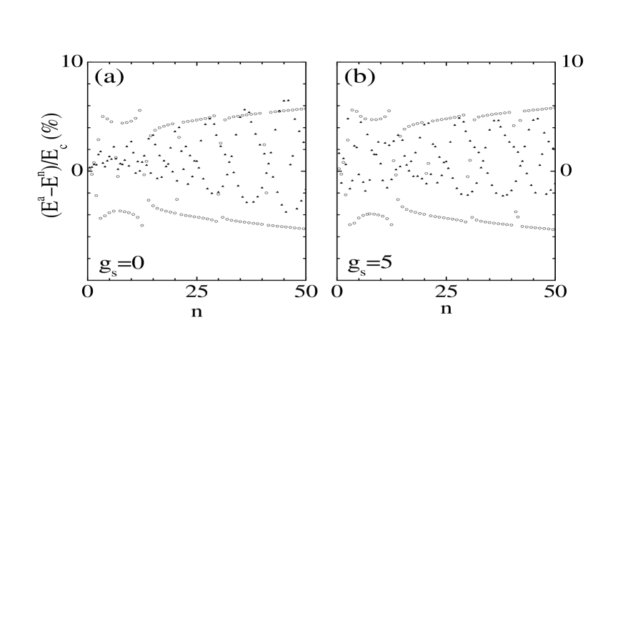
Figure 2: Energy difference between the approximate analytical $E^{a}$ and numerical $E^{n}$ results, in units of the Landau energy $E_{c}=\hbar\omega_{c}$, vs the Landau-level index $n$. The triangles show results for $\alpha=2.2\alpha_{0}$ and $\beta=1.8\alpha_{0}$, and the empty circles for $\alpha=\alpha_{0}$ and $\beta=0.2\alpha_{0}$.

To see how accurate the approximate analytical result $E^{a}$ is for higher-index subbands, which may be occupied in weak magnetic fields, in Fig. 2 we plot the energy difference $E^{a}-E^{n}$ between it and the exact numerical result $E^{n}$ normalized to the Landau energy $E_{c}=\hbar\omega_{c}$ for up to 100 levels or $n=50$ at a magnetic field $B=0.2$ T. On the average the error introduced by using the approximate result increases with the index $n$ and the SOI strength. In the absence of the Zeeman term, cf. Fig. 2(a), the approximate formula Eq. (9), corresponding to the empty circles, overestimates the subband energies of one branch while underestimates those of the other and the errors are almost proportional to the subband index $n$ for big $n$. Referring to Fig. 1, we find that the energy gap between the two branches estimated by Eq. (9) is generally narrower than it should be. The errors resulting from Eq. (16) oscillate with $n$ as $n$ increases. In a system with a $g$ factor $g_{s}=5$, as shown in Fig. 2(b), Eq. (9) is almost as accurate as for a system with $g_{s}=0$ due to the fact that the Hamiltonian Eq. (II) can be solved exactly when $\beta=0$. The error distribution range introduced by using Eq. (16) for $g_{s}=5$ shrinks compared to that for $g_{s}=0$. For $\alpha\ll\beta$ the approximate result is as precise as that for $\beta\ll\alpha$.

The density of states (DOS) is defined by $D(E)=\sum_{nk_{x}\sigma}\delta(E-E_{n}^{\sigma})$. Assuming a Gaussian broadening of constant width $\Gamma$ and zero shift we obtain

$$D(E)=\frac{S_{0}}{(2\pi)^{3/2}l_{c}^{2}\Gamma}\sum_{n,\sigma}e^{-(E-E_{n}^{\sigma})^{2}/2\Gamma^{2}}.$$ (18)

In Fig. 3(a) the DOS is plotted as function of the energy for $\alpha=\alpha_{0}$, $\beta=0$, and $g_{s}=0$ at a magnetic field $B=0.2$ T. As discussed in our previous work wang , it shows a beating pattern as a result of two branches of energy levels, i.e., the $+$ and $-$ ones, with different energy separations between the levels due to the spin splitting. The $m$th node of the beating pattern is located near the $n$th Landau level when $E^{-}_{n+m}\simeq(E^{+}_{n-1}+E^{+}_{n})/2$, which corresponds to an energy $\tilde{E}_{m}\simeq(2m+1)^{2}\hbar\omega_{c}/(4\sqrt{2}k_{\alpha}l_{c})^{2}$. For the parameters used in Fig. 3, the node energies are $0.92,2.55,5,8.26$, and $12.3$ meV for the first five nodes. For $\beta\ll\alpha$, the spin splitting between the $+$ and $-$ branches is enhanced and the node energy is reduced by a factor $1-\beta^{2}/\alpha^{2}$ as shown in Fig. 3(b). In Fig. 3(c) and (d), the DOS is shown as a function of the energy using the same parameters as in Fig. 3(a) and (b), respectively, but with a nonzero Zeeman term $g_{s}=5$. The Zeeman term does shift the levels and the DOS along the energy axis but does not affect the beating pattern substantially in the SOI regime discussed here; its effect on transport should be more visible in a weaker SOI regime. shen

Figure 3: DOS as a function of energy for $\alpha=\alpha_{0}$ with $\beta=0$ in (a) and (c) and $\beta=0.2\alpha_{0}$ in (b) and (d). The left panels are for $g_{s}=0$ and the right ones for $g_{s}=5$. In panels (b) and (d) the exact results are shown by the dotted curves and the approximate ones by the solid curves.

For $\alpha=\beta$ the energy spectrum is a series of shifted Landau levels with degenerate spinors as described by Eq. (14). The DOS appears as a series of broadened peaks with frequency $\hbar\omega_{c}$. When $\beta$ deviates little from $\alpha$, however, the degenerate spinors in each Landau subband split. As shown in Fig. 4 and described by Eq. (16), the spin splitting oscillates as a function of the subband energy or Landau index and leads to a new kind of beating pattern.

Using the asymptotic expression of the Laguerre polynomials we obtain

$$\lambda_{n}\equiv\eta_{n}/\hbar\omega_{c} \sim (2n)^{1/4}b\sqrt{2k_{s}l_{c}}\sin(4\sqrt{2n}k_{s}l_{c}-\pi/4)/(\sqrt{\pi}a)$$

$$- g_{s}\mu_{B}m^{\ast}\cos(4\sqrt{n}k_{s}l_{c}-\pi/4)/(e\hbar\sqrt{2\pi\sqrt{n}k_{s}l_{c}}).$$

When the magnetic field is weak and many Landau levels are occupied, as assumed here, the second term of Eq. (II.2) can be safely neglected. Then the zeros of $\eta_{n}$ occur for $4\sqrt{2n}k_{s}l_{c}=(p+1/4)\pi$ with $p$ integer. The spin splitting evaluated from the exact energy spectrum (zigzagged curve) and from Eq. (II.2) (smooth curve) are plotted in Figs. 4(a) and (d) for $g_{s}=0$ and $g_{s}=5$, respectively. In Fig. 4(a), the zeros of $\eta_{n}$ from Eq. (II.2) occur at $E=0.252(p+1/4)^{2}$ meV with $p=0,1,2,\cdots$. These zeros remain almost intact when the Zeeman term is considered as shown in Fig. 4(d). In Figs. 4(b) and (e) we show the exact DOS for $g_{s}=0$ and $g_{s}=5$ respectively. We find little dependence of the beating pattern on the Zeeman term. In Figs. 4(c) and (f) we plot again the DOS for $g_{s}=0$ and $g_{s}=5$, respectively, calculated from the approximate energy spectrum Eq. (16) and find a good correspondence with the exact beating pattern. The form of the beating pattern in the DOS is determined by the ratio $\lambda_{n}$ of the spin splitting $\eta_{n}$ to the Landau energy $\hbar\omega_{c}$. For $\lambda_{n}<0.5$, as shown in Fig. 4, each maximum in the DOS corresponds to a minimum in $\lambda_{n}=0$ and a minimum in the DOS to a maximum in $\lambda_{n}$. At $\lambda_{n}=0.5$ a node appears in the beating pattern while for a $\lambda_{n}$ maximum larger than $0.5$ there corresponds an extra maximum in the DOS oscillation as shown in Fig. 5. Notice that the peaks of a wrap for $\lambda_{n}<0.5$ appear at the centers of the Landau levels ${\cal E}^{\sigma}_{n}=(n+1/2)\hbar\omega_{c}-2\hbar^{2}k_{s}^{2}/m^{\ast}$ while the peaks of a wrap for $\lambda_{n}>0.5$ appear in the middle of two adjacent Landau levels ${\cal E}^{\sigma}_{n}+1/2\hbar\omega_{c}$. This DOS-peak-position transition between $\lambda_{n}<0.5$ wraps and $\lambda_{n}>0.5$ wraps leads to the even-odd filling factor transition in the SdH oscillation described in the next section.

Figure 4: SOI splitting over the Landau energy $\lambda_{n}$ ((a) and (d)), exact DOS ((b) and (e)), and approximate DOS ((c) and (f)) as functions of the energy $E$. The zigzagged curves in (a) and (d) are the exact results and the smooth curves the approximate one. The parameters are $\alpha=2.2\alpha_{0}$, $\beta=1.8\alpha_{0}$, and $B=0.2$T. The left panels are for $g_{s}=0$ and the right ones for $g_{s}=5$.

Figure 5: The same as in Fig. 4 but for $\alpha=1.2\alpha_{0}$ and $\beta=0.8\alpha_{0}$.

III Transport coefficients

For weak electric fields $E_{\nu}$, i.e., for linear responses, and weak scattering potentials the expression for the direct current (dc) conductivity tensor $\sigma_{\mu\nu}$, in the one-electron approximation, reviewed in Ref. vas2 , reads $\sigma_{\mu\nu}=$ $\sigma_{\mu\nu}^{d}+\sigma_{\mu\nu}^{nd}$ with $\mu,\nu=x,y,z$. The terms $\sigma_{\mu\nu}^{d}$ and $\sigma_{\mu\nu}^{nd}$ stem from the diagonal and nondiagonal part of the density operator $\hat{\rho}$, respectively, in a given basis and $\langle J_{\mu}\rangle=Tr(\hat{\rho}J_{\mu})=\sigma_{\mu\nu}E_{\nu}$. In general, we have $\sigma_{\mu\nu}^{d}=$ $\sigma_{\mu\nu}^{dif}+\sigma_{\mu\nu}^{col}$. The term $\sigma_{\mu\nu}^{dif}$ describes the diffusive motion of electrons and the term $\sigma_{\mu\nu}^{col}$ collision contributions or hopping. The former is given by

$$\sigma_{\mu\nu}^{dif}=\frac{\beta e^{2}}{S_{0}}\sum_{\zeta}f(E_{n}^{\sigma})[1-f(E_{n}^{\sigma})]\tau^{\zeta}(E_{n}^{\sigma})v_{\mu}^{\zeta}v_{\nu}^{\zeta},$$ (20)

where $\zeta\equiv(n,\sigma,k_{y})$ denotes the quantum numbers, $v_{\mu}^{\zeta}=\langle\zeta|v_{\mu}|\zeta\rangle$ is the diagonal element of the velocity operator $v_{\mu}$, and $f(\varepsilon)$ the Fermi-Dirac function. Further, $\tau^{\zeta}(E_{n}^{\sigma})$ is the relaxation time for elastic scattering, $\beta=1/k_{B}T$, and $S_{0}$ is the area of the system. The term $\sigma_{\mu\nu}^{col}$ can be written in the form

$$\sigma_{xx}^{col}=\frac{\beta e^{2}}{2S_{0}}\sum_{\zeta,\zeta^{\prime}}\int_{-\infty}^{\infty}d\varepsilon\int_{-\infty}^{\infty}d\varepsilon^{\prime}\delta[\varepsilon-E_{n}^{\sigma}(k_{y})]\delta[\varepsilon^{\prime}-E_{n^{\prime}}^{\sigma^{\prime}}(k_{y}^{\prime})]f(\varepsilon)[1-f(\varepsilon^{\prime})]W_{\zeta\zeta^{\prime}}(\varepsilon,\varepsilon^{\prime})(x_{\zeta}-x_{\zeta^{\prime}})^{2},$$ (21)

where $x_{\zeta}=\langle\zeta|x|\zeta\rangle$; $W_{\zeta\zeta^{\prime}}(\varepsilon,\varepsilon^{\prime})$ is the transition rate. For elastic scattering by dilute impurities, of density $N_{I}$, we have

$$W_{\zeta\zeta^{\prime}}(\varepsilon,\varepsilon^{\prime})=\frac{2\pi N_{I}}{\hbar S_{0}}\sum_{{\bf q}}|U({\bf q})|^{2}|F_{\zeta\zeta^{\prime}}(u)|^{2}\delta(\varepsilon-\varepsilon^{\prime})\delta_{k_{y},k_{y}^{\prime}-q_{y}},$$ (22)

where $u=l_{c}^{2}q^{2}/2$ and $q^{2}=q_{x}^{2}+q_{y}^{2}$. $U({\bf q})$ is the Fourier transform of the screened impurity potential $U({\bf r})=(e^{2}/4\pi\epsilon_{0}\epsilon)e^{-k_{0}r}/r$, $\epsilon$ is the static dielectric constant, $\epsilon_{0}$ the dielectric permittivity, and $k_{0}$ the screening wave vector. $U({\bf q})$ is given by

$$U({\bf q})=\frac{e^{2}}{2\epsilon_{0}\epsilon}\ \frac{1}{(2u/l_{c}^{2}+k_{0}^{2})^{1/2}}.$$ (23)

In the situation studied here the diffusion contribution given by Eq. (20) vanishes because the diagonal elements of the velocity operator $v_{\mu}^{\zeta}$ vanish. Neglecting Landau-level mixing, i. e., taking $n^{\prime}=n$, and noting that $\sigma_{xx}^{col}=\sigma_{yy}^{col}$, $\sum_{{\bf q}}=(S_{0}/2\pi)\int_{0}^{\infty}qdq=(S_{0}/2\pi l_{c}^{2})\int_{0}^{\infty}du$, and $\sum_{k_{y}}=(S_{0}/2\pi l_{c}^{2})$, we obtain

$$\sigma_{xx}^{col}=\frac{N_{I}\beta e^{2}}{2\pi\hbar l_{c}^{2}}\sum_{n\sigma}\int_{0}^{\infty}du\int_{-\infty}^{\infty}d\varepsilon[\delta(\varepsilon-E_{n}^{\sigma})]^{2}f(\varepsilon)[1-f(\varepsilon)]\left|U\left(\sqrt{2u/l_{c}^{2}}\right)\right|^{2}\left|F_{nn}^{\sigma}(u)\right|^{2}u.$$ (24)

Here $\left|F_{nn}^{\sigma}(u)\right|^{2}=|\langle f_{n}^{\sigma}|e^{i{\bf q}\cdot{\bf r}}|f_{n}^{\sigma}\ \rangle|^{2}$ is the form factor.

The form factor for $\beta=0$ has been given in Ref. wang, ; a similar form factor is obtained if $\alpha=0$ with the substitutions of the variables given in Sec. II A. For $\beta\ll\alpha$ or $\alpha\ll\beta$, the form factor is obtained in a straightforward way with the help of the above results and Eq. (9) or its $\alpha\ll\beta$ counterpart. For $\alpha\approx\beta$ the form factor reads

$$\left|F_{nn}^{\sigma}(u)\right|^{2}=e^{-u}[L_{n}(u)]^{2}\cos(\sqrt{2}q_{x}k_{s}l^{2}_{c}).$$ (25)

The exponential $e^{-u}$ favors small values of $u$. Assuming $k_{0}^{2}l_{c}^{2}/2\gg u$, we may neglect the term $2u/l_{c}^{2}$ in the denominator of Eq. (23) and obtain

$$\sigma_{yy}^{col}=\frac{N_{I}\beta e^{2}}{4\pi\hbar b}\left[\frac{e^{2}}{2\epsilon\epsilon_{0}}\right]^{2}\sum_{n\sigma}(2n+1)\int_{-\infty}^{\infty}d\varepsilon[\delta(\varepsilon-E_{n}^{\sigma})]^{2}f(\varepsilon)[1-f(\varepsilon)].$$ (26)

The impurity density $N_{I}$ determines the Landau Level broadening $\Gamma=W_{\zeta\zeta^{\prime}}(\varepsilon,\varepsilon^{\prime})/\hbar$. Evaluating $W_{\zeta\zeta^{\prime}}(\varepsilon,\varepsilon^{\prime})/\hbar$ in the $u\to 0$ limit without taking into account the SOI, we obtain $N_{I}\approx 4\pi[(2\epsilon\epsilon_{0}/e^{2})]^{2}\Gamma/\hbar$.

The resistivity tensor $\rho_{\mu\nu}$ is given in terms of the conductivity tensor. We use the standard expressions $\rho_{xx}=\sigma_{yy}/S$ and $\rho_{yy}=\sigma_{xx}/S$, with $S=\sigma_{xx}^{2}+\sigma_{yx}^{2}$. In weak magnetic fields where the beating patterns are well observed, we have $\sigma_{xy}^{nd}\approx ne/B$.

Figure 6: SdH oscillations of the conductivity $\sigma_{xx}$ in (a) and of the resistivity $\rho_{yy}$ in (b) vs inverse magnetic field $B^{-1}$ for a 2DEG with $\alpha=2.2\alpha_{0}$, $\beta=1.8\alpha_{0}$, $g_{s}=5$, and $n_{e}=8\times 10^{11}$ cm ^-2.

In weak magnetic fields a beating pattern is observed in the presence of SOI except for $\alpha=\beta$. When $\beta\ll\alpha$ the beating pattern is similar to that of $\beta=0$ as described in Ref. wang, with a period reduced by a factor $1-\beta^{2}/\alpha^{2}$. As a function of $1/B$ the period of a beating pattern for $\alpha\approx\beta$ can be estimated from the asymptotic expression of the spin splitting as $[4am^{\ast}\sqrt{2n_{e}/\pi}/e]^{-1}$. In Fig. 6 we show a periodic beating pattern in the conductivity $\sigma_{xx}$, in (a), and the resistivity $\rho_{yy}$, in (b), for a 2DEG with $\alpha=2.2\alpha_{0}$ and $\beta=1.8\alpha_{0}$. The period of the pattern is $B^{-1}=0.41$T^-1 and agrees well with the above estimate.

One interesting aspect of the beating pattern of the SdH oscillations is the even-odd filling factor transition edmo , a phenomenon in which the peaks in one wrap of the beating pattern happen at even filling factors of the 2DEG while in the next wrap occur at odd filling factors. For $\alpha\gg\beta$ or $\alpha\ll\beta$ there is always a even-odd filling factor transition between two consecutive beats. However, for $\alpha\approx\beta$ this transition occurs only for $\lambda_{n}>0.5$. In Fig. 7(a) we plot again the conductivity of Fig. 6(a) as a function of the filling factor $nh/eB$ and do not observe the even-odd transition. In Fig. 7(b) the conductivity for a system with different SOI strength $\alpha=1.2\alpha_{0}$ and $\beta=0.8\alpha_{0}$ is plotted and shows the even-odd transition. This difference can be explained using the DOS in Figs. 4 and 5. In Fig. 4, where the DOS pertaining to the parameters of Fig. 7(a) is shown, $\lambda_{n}$ is less than 0.5 and the peaks of the DOS appear at energy $\mathcal{E}_{n}^{\sigma}$ given by Eq. (14) coinciding with the Fermi energy of the 2DEG for an odd filling factor. On the other hand, in Fig. 5, where the DOS of the 2DEG pertaining to the parameters of Fig. 7(b) is shown, the peaks of the DOS occur at $\mathcal{E}_{n}^{\sigma}$ when $\lambda_{n}<0.5$ but transit to $\mathcal{E}_{n}^{\sigma}+0.5\hbar\omega_{c}$, an energy corresponding to the Fermi energy for an even filling factor and $\lambda_{n}>0.5$.

Figure 7: (a) The conductivity in Fig. 6(a) as a function of the filling factor $nh/eB$. (b) The same as in (a) for a 2DEG with $\alpha=1.2\alpha_{0}$, $\beta=0.8\alpha_{0}$, $g_{s}=5$ and $n_{e}=8\times 10^{11}$ cm ^-2.

IV concluding remarks

We studied the energy band structure, DOS, and SdH oscillations of a 2DEG in the presence of a perpendicular magnetic field and of both terms of the SOI, the Rashba (RSOI) and Dresselhaus (DSOI) terms, respectively, of strength $\alpha$ and $\beta$. Besides the exact solution of the Hamiltonian with only one of these terms present ($\alpha=0$ or $\beta=0)$, we found an exact solution for equal strengths $\alpha=\beta$ provided the Zeeman coupling is negligible. Then the band structure is just a series of spin-degenerate Landau levels shifted by the constant $2\hbar^{2}k^{2}_{s}/m^{\ast}$, cf. Eq. (13). When a difference exists between the strengths $\alpha$ and $\beta$, we obtained an approximate analytical expression for the energy spectrum and used it to study the magnetotransport of the 2DEG.

A beating pattern of the DOS and the SdH oscillations develops but with various characteristics when the ratio $\alpha/\beta$ is varied. For $\alpha\gg\beta$ or $\alpha\ll\beta$, the band structure consists of two branches of unequally spaced levels and the corresponding beating patterns of the DOS and SdH oscillations show an even-odd filling factor transition. On the other hand, for $\alpha\approx\beta$ the band structure is approximately a series of shifted Landau subbands with the spin splitting varying with subband index. As a result, the beating patterns of the DOS and of the SdH oscillations do not show any even-odd filling factor transition if the spin-splitting is less than half of the Landau energy.

References

• (1) R. Winkler, Spin-orbit coupling effects in two-dimensional electron and hole systems, Springer Tracts in Modern Phys. Vol. 191 (2003).
• (2) Y. A. Bychkov and E. I. Rashba, J. Phys. C 17, 6039 (1984).
• (3) G. Dresselhaus, Phys. Rev. 100, 580 (1955).
• (4) M. I. D’yakonov and V. Yu. Kachorovskii, Fiz. Tekh. Poluprovodn. 20, 178 (1986) [Sov. Phys. Semicond. 20, 110 (1986).
• (5) L. Vervoort, R. Ferreira, and P. Voisin, Phys. Rev. B 56, R12744 (1997).
• (6) U. Rossler and J. Kainz, Solid State Communications 121, 313 (2002).
• (7) X. F. Wang, P. Vasilopoulos, and F. M. Peeters, Phys. Rev. B 65, 165217 (2002).
• (8) J. Luo, H. Munekata and F. F. Fang, P. J. Stiles, Phys. Rev. 41, 7685 (1990).
• (9) T. Koga, J. Nitta, T. Akazaki, and H. Takayanagi, Phys. Rev. Lett. 89, 46801 (2002).
• (10) S. D. Ganichev, V. V. Bel’kov, L. E. Golub, E. L. Ivchenko, P. Schneider, S. Giglberger, J. Eroms, J. De Boeck, G. Borghs, W. Wegscheider, D. Weiss, and W. Prettl, Phys. Rev. Lett. 92, 256601 (2004).
• (11) J. J. Heremans, private communication.
• (12) J. Schliemann, J. C. Egues, and D. Loss, Phys. Rev. Lett. 90, 146801 (2003).
• (13) X. F. Wang and P. Vasilopoulos, Phys. Rev. B 67, 85313 (2003); M. Langenbuch, M. Suhrke, and U. Rossler, Phys. Rev. B 69, 125303 (2004).
• (14) J. Nitta, Y. Lin, T. Akazaki, and T. Koga, Appl. Phys. Lett. 83, 4565 (2003).
• (15) C. M. Hu, J. Nitta, T. Akazaki, H. Takayanagai, J. Osaka, P. Pfeffer and W. Zawadzki, Phys. Rev. B 60, 7736 (1999).
• (16) S. Q. Shen, M. Ma, X. C. Xie, and F. C. Zhang, Phys. Rev. Lett. 92, 256603 (2004).
• (17) P. Vasilopoulos and C. M. Van Vliet, J. Math. Phys. 25, 1391 (1984).
• (18) J. Shi, F. M. Peeters, K. W. Edmonds, and B. L. Gallagher, Phys. Rev. B 66, 35328 (2002).