Nonlinear Coupling in Nb/NbN Superconducting Microwave Resonators

Abstract

In this experimental study we show that the coupling between Nb/NbN superconducting microwave resonators and their feedline can be made amplitude dependent. We employ this mechanism to tune the resonators into critical coupling condition, a preferable mode of operation for a wide range of applications. Moreover we examine the dependence of critical coupling state on other parameters such as temperature and magnetic field. Possible novel applications based on such nonlinear coupling are briefly discussed.

Recently, there has been a growing scientific interest in nonlinear directional couplers especially in the optical regime squeezing . It has been shown in a series of publications, that operating such devices by means of parametric downconversion, may exhibit some important quantum phenomena, such as generation of quadrature-squeezed states squeezing , occurrence of quantum Zeno and anti-Zeno effects zeno , non-classical correlations EPR , and quantum entanglement entanglement . Such effects, if generated and engineered, would have immediate and significant implications on a wide range of fields, ranging from basic science to optical communication systems, and quantum computation correlated ,statics . The dependence of these mentioned effects on optimal coupling strengths and cavity detunings are almost evident squeezing ,EPR .

In this study we investigate the coupling between nonlinear NbN/Nb microwave resonators and their feedlines, as a function of injected power, ambient temperature and applied magnetic field. We show that the coupling in these resonators could be, to a large extent, dependent on externally applied parameters, allowing us thus to tune the resonators into critical coupling condition, which is a coupling state where the power transferred to the device is maximized and no power reflection is present. Such a state occurs as both impedances of the device and of the feedline match.

Theoretically critical coupling can be achieved by either tuning the coupling parameters or by altering the internal/external losses of the device. Such control was reported in optical systems Control SOA , where critical coupling was obtained in microring resonator by altering the internal loss inside the ring by means of integrated semiconductor optical amplifiers. Other critical coupling achieved in a fiber ring resonator configuration may be used in optical communication systems i.e. switches and modulators cc Yariv ,Control of cc ring-fiber conf .

Our fabricated resonators were assembled in a standard stripline geometry, and were housed in a gold plated Faraday package made of Oxygen Free High Conductivity (OFHC) Cupper. The layout of the Nb and NbN resonators are presented in the insets of Figs.4 and 2 respectively. The resonators were dc-magnetron sputtered, at room temperature, on sapphire substrates with dimensions 34$\mathrm{mm}$ X 30$\mathrm{mm}$ X 1$\mathrm{mm}$ each. A gap of 0.5 mm was set between the feedline and the resonators. The thickness of the Nb sputtered film is $2200\mathrm{\text{\AA}},$ whereas the thickness of the NbN film is $3000\mathrm{\text{\AA}}$. Following the deposition, the Nb resonator was patterned using standard photolithography process and dry etched with photo resist mask. The sputtering parameters of the NbN superconducting microwave resonator have been discussed elsewhere nonlinear features BB .

The measurements of the resonators were done using the S parameter of a vector network analyzer, while varying the input power or the ambient temperature in small steps. In Figs. 1,2 we show a power induced critical coupling data obtained at the first mode of the NbN resonator. In Fig. 1 we plot the $S_{11}\left(\omega\right)$ curves of the first mode in the complex plane, corresponding to three input powers $0.944\mathrm{mW}$, $1.072$ $\mathrm{mW}$, $1.14\mathrm{mW}$ in the vicinity of the resonance, representing $p<p_{c},$ $p=p_{c},$ $p>p_{c}$ states respectively, where $p_{c}$ is the injected power level at which critical coupling is achieved. These three trajectories show clearly that the NbN resonator at its first mode has transformed from overcoupled (strongly coupled), to undercoupled state (loosely coupled) through critically coupled condition via input power increase only. In Fig. 2 (a) we show the resonance curves $\left|S_{11}\right|$ of the three input powers, presented previously in Fig. 1, in the vicinity of the resonance. The resonances were shifted vertically for clarity. In Fig. 2 (b) we present the nonlinear evolution of the $\left|S_{11}\right|$ minimum at resonance as the input power is increased through the critical coupling power. The minimum of the graph $\sim$ $-60$ dB at $p_{c}=1.072$ $\mathrm{mW},$ corresponds to critical coupling condition where there is no power reflection. The gradual shift of the resonance frequency towards lower frequencies as the input power is increased, is plotted in Fig. 2 (c).

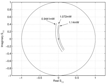
Figure 1: NbN resonator first mode $S_{11}\left(\omega\right)$ curve, drawn in the complex plane for three input powers $0.944\mathrm{mW}$, $1.072$ $\mathrm{mW}$, $1.14\mathrm{mW},$ with $2\mathrm{MHz}$ span. The resonator changes from overcoupled to undercoupled state as the power is increased through $p_{c}=1.072$ $\mathrm{mW}.$ The unit circle and the origin are also plotted on the same axis for visual comparison.

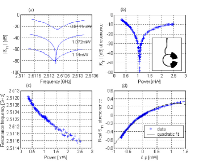
Figure 2: Data analysis of NbN  resonator first mode. (a) $\left|S_{11\text{ }}\right|$ graphs representing $p<p_{c},$ $p=p_{c}$ and $p>p_{c}$ cases. The resonance curves were shifted vertically by a constant offset for clarity. (b) $\left|S_{11\text{ }}\right|$ minimum as a function of input power. The minimum of the graph is at $p_{c}.$ (c) Resonance frequency vs. input power. (d) Real $S_{11}$ at resonance vs. power difference from critical coupling power. The resonator geometry is shown in the inset of subplot (b).

In order to identify and characterize the coupling mechanism responsible for this dependence on the drive amplitude, we apply the following universal expression for reflection amplitude of a linear resonator near resonance Yurke Eyal

$$S_{11}(\omega)=\frac{i(\omega_{0}-\omega)-(\gamma_{1}-\gamma_{2})}{i(\omega_{0}-\omega)+(\gamma_{1}+\gamma_{2})},$$ (1)

where $\gamma_{1}$ and $\gamma_{2}$ are real coupling factors associated with the feedline-resonator and the resonator-reservoir (dissipation) couplings respectively. However, unlike linear oscillators where $\gamma_{1}$, $\gamma_{2}$ and $\omega_{0}$ are constants, here we assume that these factors depend on some externally applied parameter $x,$ such as input power, temperature, and magnetic field. This generalization could be justified by noting that the $\left|S_{11}\left(\omega\right)\right|$ curves measured in the vicinity of the resonance, are to a good approximation symmetrical Lorentzians. The different possible coupling states of the resonator as described generally by Eq.(1) are shown schematically in Fig. 3.

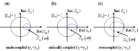
Figure 3: Resonator coupling states as defined by their $S_{11}(\omega)$ curves in the vicinity of the resonance $\omega_{0},$ (see Eq.(1)) corresponding for (a) undercoupled state (b) critically coupled state (c) overcoupled state.

By expanding $\gamma_{1}$ and $\gamma_{2}$ near critical coupling drive $x_{c},$ to lowest order in $\delta x=x-x_{c},$ we get $\gamma_{1}=\gamma+g_{1}\delta x$ and $\gamma_{2}=\gamma+g_{2}\delta x,$ where $\gamma,g_{1}$ and $g_{2}$ are real constants.

Substituting for $\gamma_{1}$ and $\gamma_{2}$ in the vicinity of $x_{c}$ in Eq.(1) at the corresponding resonance $\omega=\omega_{0},$ yields

$$S_{11}\left(\omega_{0}\right)=a_{1}\delta x+a_{2}\left(\delta x\right)^{2}+O\left(\left(\delta x\right)^{3}\right),$$ (2)

where $a_{1}=\left(g_{2}-g_{1}\right)/2\gamma,$ $a_{2}=\left(g_{1}^{2}-g_{2}^{2}\right)/4\gamma^{2}.$

In order to evaluate the critical coupling constant $\gamma$ characterizing the resonance presented earlier, we applied a fit to the resonance curve at $p_{c}$ using Eq.(1) and obtained $\gamma=1.3\mathrm{MHz}.$ Moreover, we extracted $g_{1}$ and $g_{2}$ by applying a quadratic polynomial fit as in Eq.(2) to the experimental data of real $S_{11}$ at resonance as a function of $\delta p.$ The data and the quadratic fit are presented in Fig. 2 (d), yielding the following nonlinear coupling rates $g_{1}=-0.1\mathrm{MHz}/\mathrm{mW}$, $g_{2}=1.2\mathrm{MHz}/\mathrm{mW}.$ Having $\left|g_{2}\right|>\left|g_{1}\right|$ and $g_{2}>0,$ implies that the critical coupling in this case, is caused mainly by the increase of the dissipation coupling as the input power is increased.

In the Nb resonator, power induced critical coupling was attained at $12.589\mathrm{GHz}$ resonance as shown in Fig. 4. The resonator changes from undercoupled state to overcoupled state as the power is increased through the critical coupling power at $6.59\mathrm{mW}$ . The coefficients $\gamma,g_{1},g_{2}$ extracted for this case are $48.5\mathrm{MHz},$ $1.6\mathrm{MHz}/\mathrm{mW},$ $1.5\mathrm{MHz}/\mathrm{mW}$ respectively. Implying surprisingly that what led to critical coupling in this case, is the increase of the feedline-resonator coupling at higher rate than the increase of the dissipation coupling rate, since we have $\left|g_{1}\right|>\left|g_{2}\right|$, $g_{1}>0$. Such increase in the feedline-resonator coupling could be attributed to a nonlinear redistribution of the standing-wave voltage-mode inside the resonator relative to the feedline position, leading to amplitude dependence of $\gamma_{1}.$

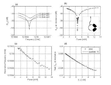
Figure 4: Data analysis of Nb resonator critical coupling at $12.589\mathrm{GHz}$ resonance. (a) $\left|S_{11\text{ }}\right|$ graphs representing $p<p_{c},$ $p=p_{c}$ and $p>p_{c}$ cases. The resonance curves were shifted vertically by a constant offset for clarity. (b) $\left|S_{11\text{ }}\right|$ minimum as a function of input power. The minimum of the graph is at $p_{c}$ . (c) Resonance frequency vs. input power. (d) Real $S_{11}$ at resonance vs. power difference $\delta p$ from critical coupling power. The resonator geometry is shown in the inset of subplot (b).

Based on our experimental demonstration of nonlinear coupling between superconducting stripline elements it is interesting to examine the feasibility of implementing some of the theoretical proposals presented in Ref. [1-6] in the microwave regime.  For that end we consider a resonator made of two stripline elements having nonlinear coupling factor $g$ between them.  The resonator is also coupled to a feed line employed for delivering the input and output signals.  Consider operating close to a resonance having angular frequency $\omega_{0}$ and damping rate $\gamma$.  A detailed analysis of this model is beyond the scope of the present letter.  However, employing dimensionality analysis and some simplifying assumptions one finds that the onset of nonlinear instability and bifurcation is expected in such a system at input power level of order $p_{NL}^{in}\cong\gamma/g$.  In the regime of operation when the input power is close to $p_{NL}^{in}$ effects such as intermodulation gain and quantum squeezing squeezing are expected to become noticeable Yurke Eyal .  Based on our results with the Nb resonator, we estimate from the experimental values of $\gamma$ and $g_{1}$ (assuming $g=g_{1}$) that such effects can be implemented with a moderate input power of order $10^{-2}\mathrm{W}$.  On the other hand, effects such as Zeno and anti-Zeno zeno require much stronger nonlinear coupling.  We estimate that in the limit of zero temperature such effects will become noticeable only when the input power becomes comparable to $p_{\varphi}^{in}\cong\gamma/\hslash\omega_{0}g^{2}$.  Again, assuming the experimental values extracted from the data of the Nb resonator, one finds $p_{\varphi}^{in}\cong 10^{12}\mathrm{W}$ - far too high for any practical implementation.  However, further analysis is required to explore other possibilities of implementing such effects in the microwave regime.

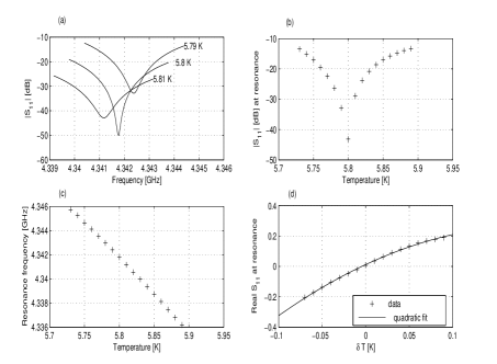
Figure 5: Data analysis of NbN second mode temperature induced critical coupling. (a) $\left|S_{11\text{ }}\right|$ graphs representing $T<T_{crit},T=T_{crit}$ and $T>T_{crit}$ cases. The resonance curves were shifted vertically by a constant offset for clarity. (b) $\left|S_{11\text{ }}\right|$ minimum as a function of temperature, the minimum of the graph is at $T_{crit}$ . (c) Resonance frequency vs. temperature. (d) Real $S_{11}$ at resonance vs. temperature difference $\delta T$ from critical coupling temperature.

In addition to input power tuning, we have succeeded to obtain critical coupling using other modes of operation, one of which was tuning the ambient temperature. To demonstrate this, we applied a constant input power to the NbN resonator and measured its second resonance response as we increased the ambient temperature in 0.01$\mathrm{K}$ steps. The input power applied was $0.1\mathrm{mW}$ , lower than $p_{c}$ of that resonance at 4.2 $\mathrm{K},$ which was about $0.209$ $\mathrm{mW}$. The resonator changed from overcoupled state at $T<T_{crit}$ to undercoupled state at $T>T_{crit}$. $T_{crit}$ was found to be 5.8$\mathrm{K}.$ The measurement results of this mode of operation are summarized in Fig. 5. By applying similar fitting procedures as was explained before one can obtain the following constants: $\gamma=4.2\mathrm{MHz},g_{1}=-0.6\mathrm{MHz}/\mathrm{K},g_{2}=220\mathrm{MHz}/\mathrm{K},$ indicating that what led to critical coupling condition, in this case, was the increase of the dissipation coupling as a result of the temperature rise.

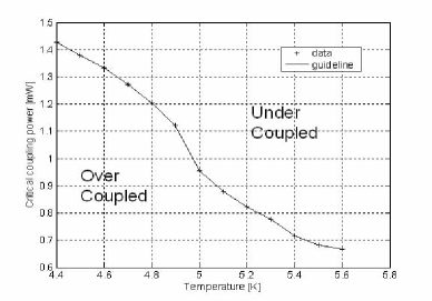
Figure 6: A plot displaying the critical coupling power dependence of the first mode of the NbN resonator on ambient temperature. The critical coupling power decreases as the temperature is increased.

Moreover to better understand the dual relation between the input power and the ambient temperature, additional measurement was carried out on the first mode of the NbN resonator. We varied the temperature of the resonator as a parameter and at each given temperature, we scanned the input power in search for the critical coupling power $p_{c}$ . The measurement result is shown in Fig. 6, where we see that in the case of the first mode of the NbN resonator at $\sim 2.5\mathrm{GHz}$, increasing the ambient temperature decreased the input power at which critical coupling occurred, and thus divided the $T-p^{in}$ plane into two regions representing the overcoupled and undercoupled resonator states, approximately separated by the guideline shown in the figure.

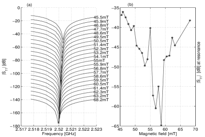
Figure 7: Critical coupling achieved by magnetic field at the first mode resonance of the NbN resonator while applying constant input power of $1.23\mathrm{mW}$. (a) $\left|S_{11}\right|$ vs. frequency corresponding to an increased applied magnetic field. The resonance curves were shifted vertically by a constant offset for clarity. (b) The $\left|S_{11}\right|$ value at the resonance frequency.

Critical coupling condition was also achieved in the NbN resonator by means of applied magnetic field. To show this we set a constant input power of $1.23\mathrm{mW}$ (the critical coupling power at the time of the measurement in the absence of magnetic field was $1.259\mathrm{mW}$), and increased a perpendicular magnetic field by small steps. The results of this mode of operation, unlike power and temperature, showed a distinct instability and frequent transitions around the critical coupling state as can be inferred from Fig. 7. A possible explanation to this instable behavior could be vortex penetration into the grain boundaries of our NbN film, as $H_{c_{1}}$ in NbN could be in the order of $35\mathrm{mT}$ nonlinear dynamics .

In summary, we have succeeded to tune our superconducting microwave resonators into critical coupling condition using input power, ambient temperature and applied magnetic field. By data fitting we have been able to extract quantitatively the coupling parameters $\gamma,g_{1},g_{2}$ and identify the dominant factor responsible for the coupling change in each case. In addition we have briefly discussed some of the possible applications of this variable coupling mechanism in exhibiting some important quantum phenomena in the microwave regime.

E.B. would especially like to thank Michael L. Roukes for supporting the early stage of this research and for many helpful conversations and invaluable suggestions. Very helpful conversations with Bernard Yurke are also gratefully acknowledged. This work was supported by the German Israel Foundation under grant 1-2038.1114.07, the Israel Science Foundation under grant 1380021, the Deborah Foundation and Poznanski Foundation.

References

- [1] A.-B. M. A. Ibrahim, B. A. Umarov, and M. R. B. Wahiddin, Phys. Rev. A 61, 043804 (2000).
- [2] J. Řehácel, J. Peřina, P. Facchi, S. Pascazi, and L. Mišta Jr., Phys. Rev. A. 62, 013804 (2000).
- [3] M. K. Olsen and P. D. Drummond, Preprint quant-ph/0412106, (2004).
- [4] J. Herec, J. Fiurášek, and L. Mišta Jr, J. Opt. B: Quant. Semiclass. Opt. 5, 419 (2003).
- [5] S. A. Podoshvedov, J. Noh, and K. Kim, Opt. Commun. 212, 115, (2002).
- [6] L. Mišta Jr., J. Herec, V. Jelínek, J. Řehácek, and J. Peřina, J. Opt. B: Quant. Semiclass. Opt. 2, 726 (2000).
- [7] V. M. Menon, W. Tong, and S. R. Forrest, IEEE Photonics Technol. lett. 16, 1343 (2004).
- [8] A. Yariv, IEEE Photonics Technol. Lett. 14, 483 (2002).
- [9] J. M. Choi, R. K. Lee and Amnon Yariv, Opt. lett. 26, 1236 (2001).
- [10] B. Abdo, E. Segev, Oleg Shtempluck, and E. Buks, arXiv:cond-mat/0501114.
- [11] B. Yurke and E. Buks, unpublished.
- [12] C. C. Chen, D. E. Oates, G. Dresselhaus and M. S. Dresselhaus, Phys. Rev. B. 45, p. 4788 (1992).