Molecular transport calculations with Wannier functions

Abstract

We present a scheme for calculating coherent electron transport in atomic-scale contacts. The method combines a formally exact Green’s function formalism with a mean-field description of the electronic structure based on the Kohn-Sham scheme of density functional theory. We use an accurate plane-wave electronic structure method to calculate the eigenstates which are subsequently transformed into a set of localized Wannier functions (WFs). The WFs provide a highly efficient basis set which at the same time is well suited for analysis due to the chemical information contained in the WFs. The method is applied to a hydrogen molecule in an infinite Pt wire and a benzene-dithiol (BDT) molecule between Au(111) surfaces. We show that the transmission function of BDT in a wide energy window around the Fermi level can be completely accounted for by only two molecular orbitals.

I Introduction

The transport of electrons in molecules plays a major role in many scientific areas. In biological systems for example electrons have to be transported to or from chemically active parts of enzymes. In electrochemistry the functioning of an electrochemical cell can be affected by the electron transport through molecular layers at the electrodes. In molecular electronics the goal is to control the electron transport in such detail that electronic components like rectifiers or transistors can be constructed from single molecules. Within these different fields a basic understanding of many phenomena related to electron transport has been obtained, but the challenge still remains to develop a detailed, quantitative approach to accurately determine the transport properties from basic quantum mechanical principles.

In this paper we address this issue in the domain where the electronic motion can be regarded as coherent. We present a numerical Green’s function method for calculating the linear response conductance of molecules and nano-contacts. The system under investigation is divided into a central scattering region and attached leads and the electronic structure of both the scattering region and the leads is described using Density Functional Theory (DFT). To represent the electronic states we use a set of localized basis functions consisting of partly occupied Wannier functions (WFs). The WFs describe the relevant states very accurately – in fact they are constructed so that they reproduce the results of high-accuracy plane-wave based pseudopotential calculations – and at the same time they represent a minimal basis set which is computationally very efficient.

In addition to their technical advantages, the Wannier functions provide insight into the local chemistry of the system and are thus well suited for analysis purposes. Being the local analogue of the extended (Bloch) states of solid state physics, the Wannier functions formalize chemical concepts such as bond types and electron lone pairs. The traditional definition of Wannier functions for single isolated bands (insulators) or occupied molecular orbitals (molecules) does not apply to metallic systems iannuzzi02 . In this case an extended scheme involving the inclusion of selected unoccupied states through a disentangling procedure must be used instead. We present a newly developed scheme which solves this problem in a simple and very direct way and we show how to link the resulting ”partly occupied WFs” to the general transport formalism through the evaluation of the relevant Hamiltonian matrices.

We apply the approach to two different systems. In the first we calculate the conductance of a hydrogen molecule suspended between two monatomic Pt wires. This can be viewed as a simple model of a recent experiment which investigated the conductance of a molecular hydrogen contact between bulk Pt electrodes smit02 . By diagonalizing the Hamiltonian within the subspace spanned by the WF of the molecule we obtain renormalized bonding and anti-bonding $\text{H}_{2}$ orbitals. The individual contributions of these orbitals to the total transmission is then studied by directly removing each of the orbitals from the basis set. In this way we find that transport is due to the anti-bonding state. The second system consists of a benzene-dithiol molecule between Au(111) surfaces. This system was among the first single-molecule systems to be studied experimentally reed97 and represents a test system for transport calculations. Our results for the conductance agree qualitatively with previous calculations, but using the analysis technique described above, we furthermore show that the transport properties of BDT can be completely accounted for by only two molecular orbitals.

The paper is organized as follows. In Sec. II we introduce the concept of phase-coherence and give an overview of existing methods for transport calculations. We then proceed to develop the general Green’s function formalism underlying the present scheme, and illustrate it through a detailed discussion of the simple case of transport through a single energy level. In Sec. III we introduce a numerical method to construct partly occupied Wannier functions and apply it to an isolated ethylene molecule and an infinite trans-polyacetylene wire. In Sec. IV we connect the Wannier functions to the general transport formalism by showing how to obtain the relevant Hamiltonian matrices in a Wannier function basis. We put emphasis on issues related to the combination of periodic supercells and transport calculations. In Sec. V we present conductance calculations for a molecular hydrogen bridge between monatomic Pt wires and a benzene-dithiol molecule suspended between Au(111) surfaces.

II Transport theory

We begin this section with a brief discussion of the phase-coherent transport regime. In order place our method in the large picture we give an overview of previously developed transport schemes. The general Green’s function formalism and the central conductance formula are then introduced in the case of non-interacting electrons moving in a static mean-field potential. Extension of the formalism to include ultrasoft pseudopotentials is shown to be straightforward. Finally, in order to illustrate the general theory we give a detailed discussion of electron transport in the simple but important Newns Anderson model.

II.1 Phase-coherent electron transport

Electron transport is said to be phase-coherent if the dimensions of the system under study are smaller than the phase relaxation length, which is the length over which the phase of an electron is randomized due to scattering datta_book ; imry_book . The phase-relaxation length thus defines the length scale on which electron interference can be observed. A typical phase relaxation length for Au at $T=1$ K is around $1\mu\text{m}$ agrait_report . In general, the phase of an electron is destroyed by interactions with the dynamic environment such as the other electrons, phonons and magnetic impurities and consequently the phase relaxation length increases at lower temperatures. Static scatterers such as the potential from the ions in a rigid lattice do not destroy the phase since the scattering is elastic and the phase change is fixed.

II.2 Existing transport schemes - an overview

During the last decade a variety of numerical methods addressing the transport of electrons in atomic-scale systems have been developed. Very generally, these methods can be divided into wave function and Green’s function methods. In both cases the description is based on a Landauer-Büttiker setup where a central scattering region is placed between two ballistic leads which are assumed to be in thermal equilibrium far from the central region.

In the wave function method one solves directly for the scattering wave functions of the system and obtain the conductance/current from the elastic transmission coefficients in accordance with the well known Landauer formula buttiker85 . The scattering states can be calculated using either the transfer matrix method sautet88 ; emberly98 ; hirose94 ; hirose95 ; choi99 ; kobayashi00 , the wave function matching method khomayakov04 or by solving a Lippman-Schwinger equation lang95 ; diventra00 . These techniques have been combined with various approximations for the electronic structure of the system, ranging from semi-empirical models like extended Hückel sautet88 ; emberly98 to fully atomistic descriptions based on the single-particle Kohn-Sham scheme of density functional theory (DFT) choi99 ; khomayakov04 . Most of the wave function methods, however, apply an intermediate level of approximation where only the electronic structure of the central region is resolved in detail while the leads are modeled by a free electron gas (jellium) hirose94 ; hirose95 ; kobayashi00 ; lang95 ; diventra00 .

As an alternative to the Landauer-Büttiker approach the transport problem can be formulated with in the non-equilibrium Green’s function formalism developed by Keldysh keldysh and Kadanoff and Baym kadanoff_baym . An advantage of the Green’s function (GF) formulation is the possibility of extending the description beyond the single-particle picture by including e.g. inelastic scattering on vibrations or correlation effects through self-energies. While the inclusion of such many-body effects is formally straightforward, the practical calculation of reliable self-energies from first principles is a difficult task which only recently has been addressed frederiksen04 . For non-interacting electrons, the GF- and Landauer-Büttiker formalisms are equivalent meirwingreen . In this case the main effort of the GF method is to calculate the GF of the central region in the presence of coupling to the leads. The effect of coupling to the leads is usually incorporated through non-hermitian self energies taylor01 ; xue01 ; brandbyge02 ; thygesen_bollinger03 ; calzolari04 ; ke04 ; heurich02 ; derosa01 ; nardelli99 ; yeyati97 ; palacios01 . The various methods mainly differ in the representation of the Hamiltonian and self-energy matrices which range from tight-binding models nardelli99 ; yeyati97 , to fully atomistic DFT descriptions taylor01 ; xue01 ; brandbyge02 ; thygesen_bollinger03 ; calzolari04 ; ke04 . Intermediate descriptions treating only the central region at the atomic level and adopting a parametrization of the coupling and lead electronic structure have also been used heurich02 ; derosa01 ; palacios01 .

The main difference among the fully DFT based GF methods lies in the basis set used to evaluate the Hamiltonian and thus the Green’s function. One limitation inherent in the GF formalism is that the basis set should consist of functions with finite support. As a consequence most methods have adopted a basis set of numerical orbitals such as Gaussians xue01 , LCAO taylor01 ; brandbyge02 ; ke04 or wavelets thygesen_bollinger03 , for which the condition of finite support can be exactly fulfilled. In contrast, there exists only a few GF transport schemes based on the more accurate plane-wave DFT methods thygesen_bollinger03 ; calzolari04 . This is partly due to the delocalized nature which excludes the plane waves themselves as basis functions and partly due to the large number of plane waves needed to perform even a small calculation with a reasonable accuracy. As we demonstrate in this paper, both of these problems can be overcome by transforming the set of pre-calculated eigenstates into an equivalent set of localized Wannier functions.

II.3 Conductance formula

We consider the phase-coherent transport of electrons through a system of the form sketched in Fig. 1. The system consists of a scattering region ($S$) connected to thermal reservoirs via left ($L$) and right ($R$) metallic leads. The reservoirs have a common temperature but different electro-chemical potentials $\mu_{L}$ and $\mu_{R}$, respectively. We shall assume that the electrons are non-interacting and move in a static mean-field potential. The leads are assumed to be perfect conductors and thus the electrons move ballistically in these regions and can scatter only on the potential inside $S$. This assumption has important computational consequences which we explore in Sec. II.4.

Figure 1: Schematic setup used to study phase-coherent electron transport. The system is divided into three regions: a scattering region ($S$) and two leads ($L$) and ($R$) connecting $S$ to thermal reservoirs with chemical potentials $\mu_{L}$ and $\mu_{R}$, respectively. The electron mean-field potential in the leads is periodic and thus all scattering takes place in $S$. Each lead can be build from a principal layer containing an integer number of potential periods.

By introducing a basis set, $\{\phi_{i}\}$, consisting of functions with finite support in the direction of transport we can decompose the underlying Hilbert space into disjoint subspaces corresponding to the three regions $S,L,R$. We do not require that the basis functions are orthogonal. The Hamiltonian matrix, $\boldsymbol{H}_{ij}=\langle\phi_{i}|H|\phi_{j}\rangle$, of the entire system takes the form

$$\boldsymbol{H}=\left(\begin{array}[]{ccc}\boldsymbol{H}_{L}&\boldsymbol{H}_{SL}^{\dagger}&0\\ \boldsymbol{H}_{SL}&\boldsymbol{H}_{S}&\boldsymbol{H}_{SR}\\ 0&\boldsymbol{H}_{SR}^{\dagger}&\boldsymbol{H}_{R}\\ \end{array}\right),$$ (1)

where the $\boldsymbol{H}_{i}$ themselves are matrices. The vanishing coupling between the leads can always be obtained by increasing the size of the scattering region, i.e. by including part of the leads in $S$. It should be noted that if the basis is not orthonormal then in general $\boldsymbol{H}$ will be different from the matrix representing the Hamiltonian in that basis.

For non-interacting electrons the retarded single particle Green’s function can be obtained from the resolvent of the Hamiltonian, $(zI-H)^{-1}$. We define the Green’s function matrix by

$$(z\boldsymbol{S}-\boldsymbol{H})\boldsymbol{G}^{r}(\varepsilon)=\boldsymbol{I},$$ (2)

where $\boldsymbol{S}_{ij}=\langle\phi_{i}|\phi_{j}\rangle$ is the overlap matrix, $\boldsymbol{I}$ the identity matrix and $z=\varepsilon+i\eta$, $\eta$ being a positive infinitesimal. To emphasize the division of the system into the three regions we write out Eq. (2) more explicitly

$$\left(\begin{array}[]{ccc}z\boldsymbol{S}_{L}-\boldsymbol{H}_{L}&z\boldsymbol{S}_{SL}^{\dagger}-\boldsymbol{H}_{SL}^{\dagger}&0\\ z\boldsymbol{S}_{SL}-\boldsymbol{H}_{SL}&z\boldsymbol{S}_{S}-\boldsymbol{H}_{S}&z\boldsymbol{S}_{SR}-\boldsymbol{H}_{SR}\\ 0&z\boldsymbol{S}_{SR}^{\dagger}-\boldsymbol{H}_{SR}^{\dagger}&z\boldsymbol{S}_{R}-\boldsymbol{H}_{R}\end{array}\right)\left(\begin{array}[]{ccc}\boldsymbol{G}_{L}^{r}&\boldsymbol{G}_{LS}^{r}&\boldsymbol{G}_{LR}^{r}\\ \boldsymbol{G}_{SL}^{r}&\boldsymbol{G}_{S}^{r}&\boldsymbol{G}_{SR}^{r}\\ \boldsymbol{G}_{RL}^{r}&\boldsymbol{G}_{RS}^{r}&\boldsymbol{G}_{R}^{r}\end{array}\right)=\left(\begin{array}[]{ccc}\boldsymbol{I}_{L}&0&0\\ 0&\boldsymbol{I}_{S}&0\\ 0&0&\boldsymbol{I}_{R}\end{array}\right),$$ (3)

It should be noted that $\boldsymbol{G}^{r}$ differs from the matrix $\langle\phi_{i}|(zI-H)^{-1}|\phi_{j}\rangle$ if the basis is not orthonormal. The two are related by

$$\langle\phi_{i}|(zI-H)^{-1}|\phi_{j}\rangle=\left[\boldsymbol{S}\boldsymbol{G}^{r}(\varepsilon)\boldsymbol{S}\right]_{ij}.$$ (4)

The Green’s function of the scattering region, $\boldsymbol{G}_{S}^{r}$, plays a central role in the theory. It can be written datta_book

$$\boldsymbol{G}^{r}_{S}(\varepsilon) = \left(z\boldsymbol{S}_{S}-\boldsymbol{H}_{S}-\boldsymbol{\Sigma}^{r}_{L}(\varepsilon)-\boldsymbol{\Sigma}^{r}_{R}(\varepsilon)\right)^{-1},$$ (5a)

$$\boldsymbol{\Sigma}^{r}_{\alpha}(\varepsilon) = \left(z\boldsymbol{S}_{S\alpha}-\boldsymbol{H}_{S\alpha}\right)\boldsymbol{g}^{0,r}_{\alpha}(\varepsilon)(z\boldsymbol{S}_{S\alpha}^{\dagger}-\boldsymbol{H}_{S\alpha}^{\dagger})$$ (5b)

$$\boldsymbol{g}_{\alpha}^{0,r}(\varepsilon) = \left(z\boldsymbol{S}_{\alpha}-\boldsymbol{H}_{\alpha}\right)^{-1},$$ (5c)

where $\alpha\in\{L,R\}$. The matrix $\boldsymbol{\Sigma}^{r}_{\alpha}$ is a non-hermitian self energy which incorporates the coupling to lead $\alpha$ and $\boldsymbol{g}_{\alpha}^{0,r}(\varepsilon)$ is the retarded Green’s function of the uncoupled lead.

An expression for the current through the system was derived by Meir and Wingreen meirwingreen using the non-equilibrium Green’s function formalism. The most general version of the formula is also valid when interactions are present in $S$. However, here we focus on the non-interacting case for which

$$I=\frac{2e}{h}\int\left[n_{\text{F}}(\varepsilon-\mu_{L})-n_{\text{F}}(\varepsilon-\mu_{R})\right]T(\varepsilon)\text{d}\varepsilon,$$ (6)

where $n_{F}(\varepsilon)$ is the Fermi distribution function and the elastic transmission function is given by

$$T(\varepsilon)=\text{Tr}\left[\boldsymbol{G}^{r}_{S}(\varepsilon)\boldsymbol{\Gamma}_{L}(\varepsilon)\boldsymbol{G}^{a}_{S}(\varepsilon)\boldsymbol{\Gamma}_{R}(\varepsilon)\right].$$ (7)

Here $\boldsymbol{G}^{a}_{S}=[\boldsymbol{G}^{r}_{S}]^{\dagger}$ denotes the advanced Green’s function of the scattering region and $\boldsymbol{\Gamma}_{\alpha}$ is obtained from the self-energies as

$$\boldsymbol{\Gamma}_{\alpha}(\varepsilon)=i\left(\boldsymbol{\Sigma}_{\alpha}^{r}(\varepsilon)-\left[\boldsymbol{\Sigma}_{\alpha}^{r}(\varepsilon)\right]^{\dagger}\right).$$ (8)

In the original derivation of Eq. (7) the basis set was assumed to be orthonormal, but in fact the formula holds for a general basis as has been shown by Xue et al. xue01 . Although the current formula (6) is valid for non-equilibrium transport we shall focus on the linear response conductance, $G$. Assuming that the difference between $\mu_{L}$ and $\mu_{R}$ is small and taking the zero temperature limit we find

$$G=G_{0}T(\varepsilon_{F}),$$ (9)

where the conductance quantum is given by $G_{0}=2e^{2}/h$.

II.4 Coupling to leads

The expression Eq. (5) for the self-energy due to lead $\alpha$ contains the Green’s function $\boldsymbol{g}_{\alpha}^{0,r}$ of the uncoupled lead. Since transport through the leads is assumed to be ballistic the electron potential must be periodic in these regions and consequently the leads can be divided into principal layers containing an integer number of potential periods. Due to the finite range of the basis functions in the transport direction, the size of the principal layers can always be chosen so large that only neighboring layers couple. In this case the Hamiltonian matrix of the left lead takes the form

$$\boldsymbol{H}_{L}=\left(\begin{array}[]{cccc}\ddots&\vdots&\vdots&\vdots\\ \ldots&\boldsymbol{h}_{0}&\boldsymbol{h}_{1}&0\\ \ldots&\boldsymbol{h}_{1}^{\dagger}&\boldsymbol{h}_{0}&\boldsymbol{h}_{1}\\ \ldots&0&\boldsymbol{h}_{1}^{\dagger}&\boldsymbol{h}_{0}\\ \end{array}\right)$$ (10)

where $\boldsymbol{h}_{0}$ is the Hamiltonian matrix of a single principal layer and $\boldsymbol{h}_{1}$ is the coupling between neighboring layers. A similar matrix structure is obtained for $\boldsymbol{H}_{R}$. In writing Eq. (10) we have assumed the lead potential to be periodic all the way up to the scattering region. This condition can always be fulfilled by extending the scattering region until it comprises all perturbations arising from the presence of scatterers. In practice such perturbations are rapidly screened by the mobile electrons in he metallic leads and the mean field potential is expected to decay to its bulk value over a few atomic layers.

The division of the leads into principal layers with nearest neighbor coupling also implies that the scattering region only couples to the principal layers immediately next to it. From Eq. (5) it then follows that only the lead Green’s function of the first principal layer is needed for evaluating the self-energy. This Green’s function can be determined iteratively due to the periodic structure of the matrix $(z\boldsymbol{S}_{\alpha}-\boldsymbol{H}_{\alpha})$. A particularly efficient iteration scheme is provided by the so-called decimation technique guinea .

II.5 Ultrasoft pseudopotentials

So far we have made no assumptions regarding the form of the mean-field electron potential. In particular it could contain non-local terms which are a natural component of most norm-conserving pseudopotentials bachelet82 ; hamann79 . However, special care must be taken when ultrasoft pseudopotentials vanderbilt90 are used, as explained below.

Suppose $H$ is an effective single-particle Hamiltonian in which the ion potential has been replaced by an ultrasoft pseudopotential. The energy spectrum is found by solving the generalized eigenvalue equation

$$H\psi_{n}=\varepsilon_{n}S\psi_{n},$$ (11)

where the pseudo wave functions satisfy the generalized orthonormality condition

$$\langle\psi_{n}|S|\psi_{m}\rangle=\delta_{nm}.$$ (12)

Although the Hamiltonian is hermitian its eigenvalues do not coincide with the real energy spectrum and it is therefore not obvious at the outset how to define the Green’s function entering the transmission formula (7).

The operator $\widetilde{H}=S^{-1}H$ has the correct spectrum but it is not hermitian - its eigenvectors are not orthogonal. This is, however, not a real problem since self-adjointness depends on the inner product. In fact $\widetilde{H}$ is hermitian if we use the inner product $\langle\cdot|\cdot\rangle_{1}$ defined by $\langle\psi|\phi\rangle_{1}=\langle\psi|S|\phi\rangle$. That $\langle\cdot|\cdot\rangle_{1}$ does define an inner product follows from the fact that $S$ is hermitian and positive in the sense $\langle\phi|S|\phi\rangle\geq 0$ for all $\phi$.

The apparent problem related to the use of ultrasoft pseudopotentials can thus be removed by changing the inner product from $\langle\cdot|\cdot\rangle$ to $\langle\cdot|\cdot\rangle_{1}$ and using the Hamiltonian $\widetilde{H}$ instead of $H$. A direct application of Eq. (2) leads to the following defining equation for $\boldsymbol{G}^{r}$:

$$(z\boldsymbol{S}-\boldsymbol{H})^{-1}\boldsymbol{G}^{r}(\varepsilon)=\boldsymbol{I},$$ (13)

where $\boldsymbol{S}_{ij}=\langle\phi_{i}|S|\phi_{j}\rangle$ and $\boldsymbol{H}_{ij}=\langle\phi_{i}|H|\phi_{j}\rangle$. Consequently, the only change in the formalism introduced by the use of ultrasoft pseudopotentials is the substitution of the ordinary overlap matrix $\langle\phi_{i}|\phi_{j}\rangle$ by the generalized overlap $\langle\phi_{i}|S|\phi_{j}\rangle$.

II.6 Newns Anderson model

In order to illustrate the use of the general formalism introduced above and to develop a physical understanding of the conductance formula (7), we discuss the case of transport through a single energy level coupled to continuous bands. As we shall see later this model is also useful for analysis and interpretation of the transport properties of more complicated systems.

In the Newns Anderson model newns69 we consider the single site $|a\rangle$ of energy $\varepsilon_{a}$ coupled to infinite leads via the matrix elements $t_{\alpha\nu}=\langle a|H|\alpha\nu\rangle$, where $\{|\alpha\nu\rangle\}$ is a basis of lead $\alpha$. The single level constitutes the scattering region and thus all matrix quantities in the transmission function (7) reduce to complex numbers. The Green’s function reads

$$G_{a}(\varepsilon)=\frac{1}{\varepsilon-\varepsilon_{a}-\Sigma_{L}(\varepsilon)-\Sigma_{R}(\varepsilon)},$$ (14)

with the self-energy due to lead $\alpha$ given by

$$\Sigma_{\alpha}(\varepsilon)=\sum_{\nu\mu}t_{\alpha\mu}(g^{0}_{\alpha})_{\mu\nu}t_{\alpha\nu}^{*},$$ (15)

We have dropped the $r$ superscripts since we consider only retarded Green’s functions in the following. A particularly elegant solution to the problem can be obtained by introducing the normalized group orbital of lead $\alpha$:

$$|\gamma_{\alpha}\rangle=V_{\alpha}^{-1}\sum_{\nu}t_{\alpha\nu}|\alpha\nu\rangle,$$ (16)

where $V_{\alpha}=(\sum_{\nu}|t_{\alpha\nu}|^{2})^{1/2}$. The group orbital is located on lead $\alpha$ and its weight on a given lead state is determined by the magnitude of the corresponding coupling matrix element. Consequently, the group orbital is expected to be localized at the lead-level interface. The coupling between $|a\rangle$ and any state in the lead orthogonal to $|\gamma_{\alpha}\rangle$ vanishes and thus $|a\rangle$ is coupled to the lead via the group orbital only, the coupling being given by $V_{\alpha}$. For simplicity we assume a symmetric contact and therefore suppress the $\alpha$ index. Using the general relation between a diagonal element of the retarded Green’s function and the projected density of states (DOS) for the corresponding orbital: $\text{Im}[G_{\nu\nu}]=-\pi\rho_{\nu}$, we can express $\Gamma$ (as defined in Eq. (8)) by the DOS for the isolated lead projected onto the group orbital: $\Gamma=\pi|V|^{2}\rho^{0}_{\gamma}$. Applying the same rule to the Green’s function of the level we arrive at

$$T(\varepsilon)=2\pi^{2}|V|^{2}\rho_{a}(\varepsilon)\rho^{0}_{\gamma}(\varepsilon).$$ (17)

This formula shows that the transmission at a given energy depends on three quantities: the coupling strength, $V$, the level DOS, $\rho_{a}$, and the DOS of the group orbital in the isolated lead, $\rho_{\gamma}^{0}$. Thus, for an electron with energy $\varepsilon$ to propagate through the system there should be states of that energy available in the leads as well on the level and the coupling should be reasonably strong.

An even simpler description is obtained in the so called wide band limit where $\rho_{\gamma}^{0}$ is assumed to be constant. In this case the transmission is usually expressed in terms of $\Gamma$ and $\varepsilon_{a}$ and reads

$$T(\varepsilon)=\frac{\Gamma^{2}}{(\varepsilon-\varepsilon_{a})^{2}+\Gamma^{2}}.$$ (18)

This is a Lorentzian of unit height and center $\varepsilon_{a}$. Its width is given by $\Gamma$ which also determines the width of the energy distribution of $|a\rangle$ in the coupled system and thus equals the inverse lifetime of an electron on the level. From this expression it is clear that the position of the Fermi level relative to $\varepsilon_{a}$ is a crucial parameter for the conductance. Finally, we note that deviations from the simple Lorentzian form (18) are expected when the coupling is asymmetric or when $\rho_{\gamma}^{0}(\varepsilon)$ has a significant energy dependence.

III Wannier Functions

In this section we present a scheme to construct partly occupied Wannier Functions (WFs)thygesen_wannier . After a brief motivation we outline the construction algorithm for both isolated and periodic systems. It is natural to introduce the algorithm first in the simpler case of an isolated system before extending it to periodic systems, although the latter contains the former as a special case. For later use we establish an expression for the matrix elements of the Hamiltonian in the WF basis. Finally, we illustrate the method by constructing the WFs for an isolated ethylene molecule and an infinite trans-polyacetylene wire.

III.1 Why Wannier functions?

There are several advantages of using WFs as a basis set for transport calculationscalzolari04 : (i) the WFs are spatially localized which allows for the necessary division into scattering region and leads. (ii) any eigenstate below a certain specified energy can, by construction, be exactly reproduced as a linear combination of the WFs and thus the accuracy of the original electronic structure calculation is retained. (iii) the WF basis set is truly minimal and once constructed the computational cost of the subsequent transport calculation is comparable to that of semi-empirical methods like tight-binding or extended Hückel. (iv) the WFs contain information about chemical properties such as bond types, coordination and electron lone pairs and can thus be directly used as an analysis tool.

The WFs are defined as linear combinations of a fixed set of single-particle eigenstates - traditionally the occupied states - with the expansion coefficients optimized to give the best localization of the resulting WFs. In this paper we shall focus on partly occupied WFs. The term ”partly occupied” refers to the fact that we allow selected unoccupied orbitals in the expansion of the WFs. In some situations this can improve the symmetry of the resulting orbitals, however, the crucial property that distinguish the partly occupied WFs from the traditional occupied WFs and make them applicable for transport calculations is that they can be localized in metallic systems. It is well known that occupied WFs associated with a partly filled band in a metal have poor localization properties souza01 ; iannuzzi02 . The only remedy for this is to include the appropriate unoccupied states in the localization space.

III.2 Isolated systems

Consider an isolated system, for which an electronic structure calculation produces $N$ eigenstates, $\{\psi_{n}\}$, of which $M$ have an energy below $E_{0}$. Our aim is to construct a set of localized orbitals out of the $\{\psi_{n}\}$, which span at least the $M$ eigenstates below $E_{0}$. We will allow eigenstates with energy above $E_{0}$ in the expansion of the WFs in order to improve the localization.

Before we can start to study localized orbitals, we need a measure for the degree of localization. Here we follow Marzari and Vanderbilt marzari97 and measure the spread of a set of functions, $\{w_{n}\}$, by the sum of second moments:

$$\mathcal{S}=\sum_{n=1}^{N}(\langle w_{n}|r^{2}|w_{n}\rangle-\langle w_{n}|\mathbf{r}|w_{n}\rangle^{2}).$$ (19)

We expand the WFs in terms of the $M$ lowest eigenstates and $L$ extra degrees of freedom, $\{\phi_{l}\}$, from the remaining $(N-M)$-dimensional eigen-subspace. This will lead to a total of $M+L$ WFs. The expansion takes the form

$$w_{n}=\sum_{m=1}^{M}U_{mn}\psi_{m}+\sum_{l=1}^{L}U_{M+l,n}\phi_{l},$$ (20)

where the extra degrees of freedom (EDF) are written as

$$\phi_{l}=\sum_{m=1}^{N-M}c_{ml}\psi_{M+m}.$$ (21)

The columns of the matrix ${c}$ are taken to be orthonormal and represent the coordinates of the EDF with respect to the eigenstates with energy above $E_{0}$. The matrix $U$ is unitary and represents a rotation in the space of the functions $\{\psi_{1},\ldots,\psi_{M},\phi_{1},\ldots,\phi_{L}\}$. It should be noticed that the construction (20) ensures that the $M$ lowest eigenstates are contained in the space spanned by the WFs. Through the expansions (20) and (21), $\mathcal{S}$ becomes a function of $U_{ij}$ and $c_{ij}$, which must be minimized under the constraint that $U$ is unitary and the columns of $c$ are orthonormal. The minimization can be performed by evaluating the derivatives of $\mathcal{S}$ with respect to $U_{ij}$ and $c_{ij}$ and then using any gradient based optimization scheme to iteratively find the minimum.

III.3 Ethylene, $\text{C}_{2}\text{H}_{4}$

To illustrate the method we have constructed the WFs of an isolated ethylene molecule. We use a cubic supercell of length 14 Å and sample the BZ by the $\Gamma$ point. In Fig. 2 we show iso-surfaces for two different sets of WFs corresponding to fully occupied WFs (upper row) generated with $E_{0}=E_{F}$ and $L=0$ and partly occupied WFs generated with $E_{0}=E_{F}$ and $L=1$. In both cases we obtain four equivalent $\sigma$-orbitals located at the C-H bonds. In contrast, the WFs describing the C-C bond changes from two equivalent orbitals with a mixed $\sigma/\pi$ character, to a single $\sigma$ orbital centered between the C atoms and two atomic-like $p$-orbitals centered on each C. By inspection we find that the EDF selected in the minimization procedure in the latter case coincide with the anti-bonding molecular $\pi$-orbital of the C-C bond. Inclusion of this orbital is precisely what is needed to separate the $\sigma$- and $\pi$-systems on the molecule.

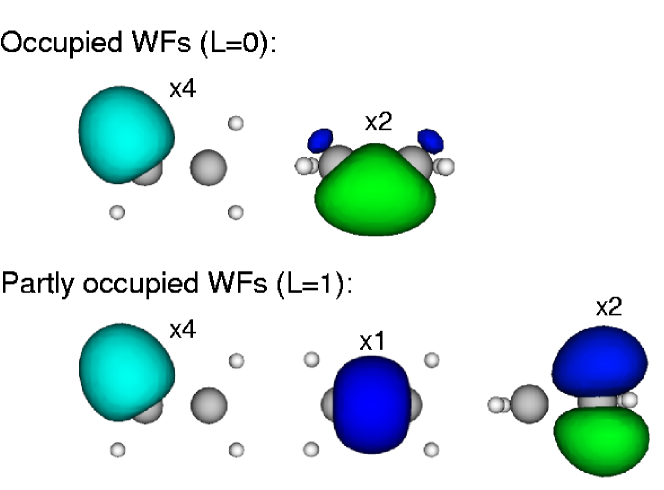
Figure 2: Occupied WFs (upper row) and partly occupied WFs (lower row) for ethylene, $\text{C}_{2}\text{H}_{4}$. The symbol $\times n$ indicate the number of similar WFs obtained at equivalent sites on the molecule. Note, that by including the anti-bonding $\pi$ orbital in the WF expansion the $\sigma$- and $\pi$-systems become separated.

III.4 Periodic systems

We now turn to the construction of WFs for a periodic system. Suppose that $\{w_{n}\}$ is a set of periodic functions defined in a cubic cell of length $a$. It has been shown that in the limit of large $a$, minimizing the spread (19) is equivalent to maximizing the functional resta99

$$\Omega=\sum_{n}(|X_{nn}|^{2}+|Y_{nn}|^{2}+|Z_{nn}|^{2}),$$ (22)

where the matrix ${X}$ is defined as

$$X_{nm}=\langle w_{n}|e^{-i(2\pi/a)x}|w_{m}\rangle,$$ (23)

with similar definitions for $Y_{nm}$ and $Z_{nm}$. The generalization to cells of arbitrary shape is straightforward and can be found in Refs. [silvestrelli98, ; berghold00, ]. Since an isolated system can always be studied in a large periodic supercell within the $\Gamma$-point approximation, the functional $\Omega$ can also be used instead of $\mathcal{S}$ to construct the WFs of a finite system.

Since $\Omega$ corresponds to $\mathcal{S}$ only for periodic functions in large supercells it seems to be useful only for systems that can be treated within the $\Gamma$-point approximation. However, by using the folding properties of the Brillouin zone (BZ) this problem can easily be overcome. Consider a periodic system with a unit cell defined by the basis vectors $\mathbb{a}_{1},\mathbb{a}_{2},\mathbb{a}_{3}$. The union of the $\mathbb{k}$-subspaces associated with a uniform $N_{1}\times N_{2}\times N_{3}$ grid in the 1.BZ which includes the $\Gamma$-point coincides with the $\Gamma$-subspace of the repeated unit cell defined by basis vectors $\mathbb{A}_{i}=N_{i}\mathbb{a}_{i}$. Consequently, any function which can be written as a sum of functions each characterized by a $\mathbb{k}$ from such a uniform grid is periodic in the repeated cell and its spread can be defined by $\Omega$. In this case the matrix elements (23) should be evaluated over the repeated cell, however, as usual this can be reduced to integrals over the small cell. Finally, we note that since the number of $\mathbb{k}$-points determines the size of the repeated cell, the original condition that the supercell should be sufficiently large is turned into a condition of a sufficiently dense $\mathbb{k}$-point sampling.

As for the non-periodic case, we start from a set of single-particle eigenstates, $\{\psi_{n\mathbb{k}}\}$, obtained from a conventional electronic structure calculation. For a periodic system, the eigenstates are Bloch states labeled by a band index, $n$, and a wave vector, $\mathbb{k}$. In accordance with the remarks above the $\mathbb{k}$-points should belong to a uniform grid which includes the $\Gamma$-point. We denote the total number of bands used in the calculation by $N$, the desired number of WFs per unit cell by $N_{w}$ and the number of eigenstates at a given $\mathbb{k}$-point with energy below $E_{0}$ by $M_{\mathbb{k}}$. If $M_{\mathbb{k}}>N_{w}$, we set $M_{\mathbb{k}}=N_{w}$. As in the isolated case, all eigenstates with energy less than $E_{0}$ will be contained in the space spanned by the WFs. We define the $n$th Wannier function belonging to cell $i$ by

$$w_{i,n}=\frac{1}{\sqrt{N_{k}}}\sum_{\mathbb{k}}e^{-i\mathbb{k}\cdot\mathbb{R}_{i}}\tilde{\psi}_{n\mathbb{k}},$$ (24)

where $N_{k}$ is the total number of $\mathbb{k}$-points and $\tilde{\psi}_{n\mathbb{k}}$ is a generalized Bloch state to be defined below. We wish to find the set of generalized Bloch states that minimizes the spread of the resulting Wannier functions. Since $w_{i,n}(\mathbb{r})=w_{0,n}(\mathbb{r}-\mathbb{R}_{i})$ it is sufficient to consider only the Wannier functions of the cell at the origin. For each of the generalized Bloch states we follow closely the idea used in the isolated case. Thus we expand $\tilde{\psi}_{n\mathbb{k}}$ in terms of the $M_{\mathbb{k}}$ lowest eigenstates and $L_{\mathbb{k}}=N_{w}-M_{\mathbb{k}}$ EDF, $\{\phi_{l\mathbb{k}}\}$, from the remaining space of Bloch states:

$$\tilde{\psi}_{n\mathbb{k}}=\sum_{m=1}^{M_{\mathbb{k}}}U(\mathbb{k})_{mn}\psi_{m\mathbb{k}}+\sum_{l=1}^{L_{\mathbb{k}}}U(\mathbb{k})_{M_{\mathbb{k}}+l,n}\phi_{l\mathbb{k}},$$ (25)

where the unoccupied orbitals are written as

$$\phi_{l\mathbb{k}}=\sum_{m=1}^{N-M_{\mathbb{k}}}c(\mathbb{k})_{ml}\psi_{M_{\mathbb{k}}+m,\mathbb{k}}.$$ (26)

Since the states $\{\psi_{n\mathbb{k}}\}$ coincide with the $\Gamma$-point eigenstates of the repeated unit cell we can use $\Omega$ to measure the spread of $w_{0,n}$. The maximization of $\Omega$ with respect to $U(\mathbb{k})_{ij}$ and $c(\mathbb{k})_{ij}$ is performed in complete analogy with the isolated case. For small systems ($\lesssim$ 10 atoms) the method is quite stable and usually leads to the same global maximum independent of the initial guess used for the matrices $U(\mathbb{k})$ and $c(\mathbb{k})$. In such cases the matrices can simply be initialized randomly. For larger systems, the method can get stuck in local maxima and we have found it useful to start the maximization from an initial guess of simple orbitals located either at the atoms or the bond centers.

III.5 Wannier function Hamiltonian

The transformation of eigenstates into localized WFs induces a transformation of the Hamiltonian from its diagonal spectral representation into a real-space or tight-binding like representation. This real-space form of the Hamiltonian is in itself very convenient as it provides direct access to physical parameters for e.g. tight-binding models.

By combining Eqs. (24,25,26) the $n$th WF located in the unit cell at $\mathbb{R}_{i}$ can be compactly written as

$$w_{i,n}=\frac{1}{\sqrt{N_{k}}}\sum_{\mathbb{k},m}e^{-i\mathbb{k}\mathbb{R}_{i}}V(\mathbb{k})_{mn}\psi_{m\mathbb{k}},$$ (27)

where $V(\mathbb{k})$ can be expressed in terms of $U(\mathbb{k})$ and $c(\mathbb{k})$. The Hamiltonian matrix element connecting the $n$th WF of cell $i$ with the $m$th WF of cell $j$ then becomes

$$H(\mathbb{R}_{j}-\mathbb{R}_{i})_{nm} \equiv \langle w_{i,n}|H|w_{j,m}\rangle$$

$$= \sum_{\mathbb{k},l}e^{-i(\mathbb{R}_{j}-\mathbb{R}_{i})\cdot\mathbb{k}}V^{*}(\mathbb{k})_{ln}V(\mathbb{k})_{lm}\varepsilon_{l\mathbb{k}}$$

where $\varepsilon_{l\mathbb{k}}=\langle\psi_{l\mathbb{k}}|H|\psi_{l\mathbb{k}}\rangle$ are the eigenvalues. Recall, that the WFs as defined here are periodic functions with a period given by the repeated cell. This periodicity is reflected in $H(\mathbb{R}_{j}-\mathbb{R}_{i})_{nm}$. In order to describe fully localized functions the coupling matrix elements must therefore be truncated beyond a cut-off distance given approximately by $N_{i}/2$ unit cells in the direction $\mathbb{a}_{i}$. This means in turn that the repeated cell should be large enough, or equivalently that the number of $\mathbb{k}$-points should be large enough, that the WFs have decayed sufficiently between the repeated images.

To test the accuracy of the transformed WF Hamiltonian we can use it to reproduce the original band structure. To this end we form the Bloch basis

$$\chi_{n\mathbb{k}}=\frac{1}{\sqrt{N_{R}}}\sum_{\mathbb{R}_{i}}e^{i\mathbb{R}_{i}\cdot\mathbb{k}}w_{i,n},$$ (29)

where $N_{R}$ is the number of unit cells included in the sum. The Hamiltonian matrix, $H(\mathbb{k})$, in the Bloch basis for a given $\mathbb{k}$ becomes

$$\langle\chi_{n\mathbb{k}}|H|\chi_{m\mathbb{k}}\rangle=\sum_{\mathbb{R}_{j}}e^{i\mathbb{k}\cdot\mathbb{R}_{j}}H(\mathbb{R}_{j})_{nm}.$$ (30)

The dimension of this matrix equals the number of WFs in one unit cell and can be easily diagonalized yielding the approximate eigenvalues $\tilde{\varepsilon}_{n\mathbb{k}}$. The quality of the eigenvalues depends on the number of cells included in the sum (30), i.e. on the range beyond which the coupling is truncated. Since $H(\mathbb{R}_{j})_{nm}$ becomes incorrect beyond $N_{i}/2$ unit cells in direction $\mathbb{a}_{i}$ the quality of the eigenvalues $\tilde{\varepsilon}_{n\mathbb{k}}$ ultimately depends on the number of $\mathbb{k}$-points used in the construction of the WFs.

III.6 Trans-Polyacetylene

As an example of a Wannier function analysis for a periodic system we have constructed the WFs of trans-polyacetylene and generated the band diagram using the corresponding WF Hamiltonian. We use a unit cell containing two carbon and two hydrogen atoms and with a large amount of vacuum separating the repeated wires by more than $10$ Å in the directions perpendicular to the wire. We use a uniform $31\times 1\times 1$ $\mathbb{k}$-point grid in the construction of the WFs. The band diagram of the wire obtained directly from the electronic structure calculation is shown in Fig. 3 (full lines). For transport calculations we need a good description of the electronic structure of the wire in an energy window around the Fermi level, $\varepsilon_{F}=0$. Thus, in addition to the filled bands we should describe at least the lower part of the $\pi^{*}$ conduction band correctly. Fig. 4 shows iso-surfaces of three different WFs obtained using the parameters $N_{w}=6$ and $E_{0}=1.0$ eV. With this choice of parameters we obtain six WFs per unit cell and ensure a correct description of the band structure up to 1.0 eV. In total we obtain a $\sigma$-orbital at every C-H and C-C bond and an atomic-like $p_{z}$-orbital centered on each C atom. It is instructive to calculate the band structure of the wire using these WFs as basis functions as described in section III.5. The result is shown by dots in Fig. 3. As expected the reconstructed bands are in good agreement with the original bands below $E_{0}$. The high density of bands starting around 3 eV above $\varepsilon_{F}$ marks the beginning of the continuous spectrum. The fact that the reconstructed $\pi^{*}$ band does not follow a particular band in this region indicates that the corresponding generalized Bloch states (25) consist of non-trivial linear combinations of delocalized original bands. This is sometimes referred to as band-disentanglement.

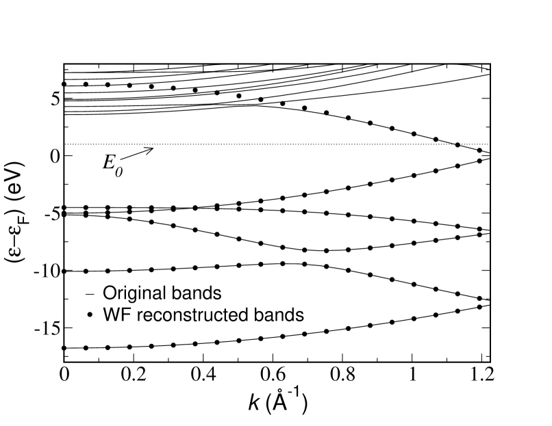
Figure 3: Comparison between the band diagram obtained directly from the electronic structure calculation (full line) and the approximate band structure obtained using the WFs of Fig. 4 as basis functions.

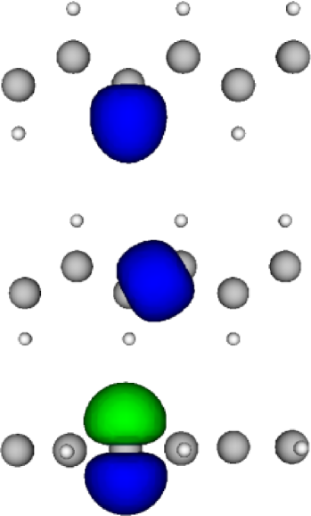
Figure 4: Partly occupied WFs for trans-polyacetylene. The unit cell contains two CH units. The WFs have been generated with the parameters $N_{w}=6$ and $E_{0}=1.0$ eV, where the Fermi level is set to 0 eV. There is one $\sigma$ orbital at every C-H and C-C bond and one atomic-like $p_{z}$ orbital on each C.

IV Representation of the Hamiltonian

In this section we link the WFs introduced in section III to the general transport formalism of section II. What is needed is a method to construct the Hamiltonian (1) for the coupled $L$-$S$-$R$ system in a localized WF basis set, and we will discuss a way of achieving this. After a general discussion of some issues related to the use of supercells in connection with transport calculations we discuss the construction of the three Hamiltonians $H_{\alpha},H_{S},H_{S\alpha}$.

IV.1 Periodic supercells

Within the periodic supercell approach, the system of interest is defined inside a finite computational cell, the supercell, which is repeated in all directions to form a super lattice. The principle is illustrated in Fig. 5 for a single molecule suspended between infinitely extended surfaces. Clearly, we must require that the transverse dimensions of the supercell as well as the thickness of the surface slabs are so large that the periodically repeated molecules do not interact.

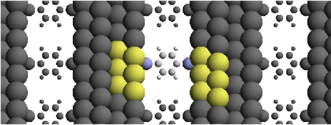
Figure 5: Illustration of a supercell describing a single molecule suspended between infinite surfaces.

Fig. 5 shows an example of a scattering region as defined in the transport setup sketched in Fig 1. If the surface slabs are thick enough, the electron density and thus the electron mean field potential at the supercell end-planes are close to their bulk values. It is therefore permissible to extend the electron potential to the left and right of the supercell by the bulk potential which leads to the system shown in Fig. 6. We note, that the system remains periodic in the directions perpendicular to the transport direction. Within this approach, we are therefore effectively considering transport through an infinite array of contacts. Whether this provides a good description of transport through a single, isolated contact then depends on the degree of interference between the repeated contacts. As the transverse dimensions of the supercell are increased this interference is expected to decrease and the result should approach that of a single contact.

Since the scattering region of the system shown in Fig. 6 consists of an infinite array of molecules, all matrices entering the transmission formula (7) have infinite dimensions. However, the periodicity of the system implies that the wave vectors, $\mathbb{k}_{\perp}$, belonging to the 1.BZ. of the transverse plane are good quantum numbers. Consequently, all the matrices entering Eq. (7) are diagonal with respect to $\mathbb{k}_{\perp}$ and the total transmission can thus be decomposed into a sum over $\mathbb{k}_{\perp}$-dependent transmissions given by

$$T(\mathbb{k}_{\perp};\varepsilon)=\text{Tr}\left[\boldsymbol{G}_{S}^{r}(\mathbb{k}_{\perp};\varepsilon)\boldsymbol{\Gamma}_{L}(\mathbb{k}_{\perp};\varepsilon)\boldsymbol{G}^{a}_{S}(\mathbb{k}_{\perp};\varepsilon)\boldsymbol{\Gamma}_{R}(\mathbb{k}_{\perp};\varepsilon)\right].$$ (31)

The transmission per supercell is evaluated as $T(\varepsilon)=\sum_{\mathbb{k}_{\perp}}W_{\mathbb{k}_{\perp}}T(\mathbb{k}_{\perp};\varepsilon)$, where $W_{\mathbb{k}_{\perp}}$ are appropriate weight factors adding up to 1.

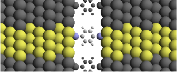
Figure 6: The system obtained by extending the electron potential to the left and right of the supercell shown in Fig. 5 by the bulk potential. Note, that the system remains periodic in the directions perpendicular to the transport direction.

IV.2 Some notation

For use in the following we introduce some notation. We take the direction of transport to coincide with the $z$-axis. For any system of the form illustrated in Figs. 5,6 we denote the basis vectors of the super lattice in the transverse plane by $\mathbb{A}_{1}$ and $\mathbb{A}_{2}$. We assume that this plane is perpendicular to the transport direction, i.e. $\mathbb{A}_{1}\cdot\mathbb{e}_{z}=\mathbb{A}_{2}\cdot\mathbb{e}_{z}=0$, and refer to the unit cell spanned by $\mathbb{A}_{1}$ and $\mathbb{A}_{2}$ as the transverse cell. A general lattice vector within this plane is denoted by $\mathbb{R}_{\perp}$, and can thus be written $\mathbb{R}_{\perp}=n\mathbb{A}_{1}+m\mathbb{A}_{2}$, where $n,m$ are integers. Finally, we denote the wave-vectors in the 1.BZ of the transverse cell by $\mathbb{k}_{\perp}$.

IV.3 Lead Hamiltonian ($\boldsymbol{H}_{\alpha}$)

In the following we describe how to construct the Hamiltonian matrix, $\boldsymbol{H}_{\alpha}$, for lead $\alpha$. From Eq. (10) it is clear that we need the matrices $\boldsymbol{h}_{0}$ and $\boldsymbol{h}_{1}$ describing a single principal layer and the coupling between two neighboring layers, respectively.

Suppose that a single principal layer of lead $\alpha$ is described by a supercell with basis vectors $\mathbb{A}_{i}=N_{i}\mathbb{a}_{i}$, $i=1,2,3$. If $N_{i}>1$ for some $i$, the principal layer can be build from a smaller unit cell with basis vectors $\mathbb{a}_{1},\mathbb{a}_{2},\mathbb{a}_{3}$. In the example illustrated in Fig. 5 a possible principal layer super cell consists of one ABC period of $3\times 3$ sections of the (111) atomic planes of the bulk fcc crystal. This cell can in turn be made up of smaller cells containing only $1\times 1$ sections in the transverse plane. Let $\{w_{i,n}\}$, $n=1,\ldots,N_{w}$ denote the set of WFs obtained for the small cell at $\mathbb{R}_{i}$. For a given $\mathbb{k}_{\perp}$ we form the Bloch functions

$$\chi_{i,n}(\mathbb{k}_{\perp})=\frac{1}{\sqrt{N_{R_{\perp}}}}\sum_{\mathbb{R}_{\perp}}e^{i\mathbb{k}_{\perp}\cdot\mathbb{R}_{\perp}}w_{i,n}(\mathbb{r}-\mathbb{R}_{\perp}),$$ (32)

where $N_{R_{\perp}}$ is the number of transverse cells included in the sum and $i$ denotes a small unit cell. Note, that even though the Bloch functions are extended in the transverse directions they preserve the finite range of the WFs in the transport direction. The corresponding Hamiltonian matrix is given by

$$H(\mathbb{k}_{\perp})_{in,jm} \equiv \langle\chi_{i,n}(\mathbb{k}_{\perp})|H|\chi_{j,m}(\mathbb{k}_{\perp})\rangle$$ (33)

$$= \sum_{\mathbb{R}_{\perp}}e^{i\mathbb{k}_{\perp}\cdot\mathbb{R}_{\perp}}H(\mathbb{R}_{j}-\mathbb{R}_{i}+\mathbb{R}_{\perp})_{nm},$$

where the matrix elements $H(\mathbb{R}_{j}-\mathbb{R}_{i}+\mathbb{R}_{\perp})_{nm}$ refer to the WF Hamiltonian of Eq. (III.5). To obtain the matrix $\boldsymbol{h}_{0}$ we let $i,j$ run over all small unit cells within one principal layer supercell and $n,m$ run over all WFs. To obtain $\boldsymbol{h}_{1}$ we do the same except that $j$ now runs over all small unit cells within the supercell of the neighboring principal layer. The accuracy of the Hamiltonian $\boldsymbol{H}(\mathbb{k}_{\perp})$ depends on the number of transverse cells included in the sum. As explained in sec. III.5 this number is limited by the size of the period of the WFs which in turn is determined by the number of $\mathbb{k}$-points used to construct them. For a transverse cell containing $3\times 3$ atoms we have found it sufficient to sum over nearest neighbor cells.

IV.4 Hamiltonian for scattering region ($\boldsymbol{H}_{S}$) and coupling ($\boldsymbol{H}_{S\alpha}$)

The technique for constructing a matrix representation of the lead Hamiltonian described in the previous section can also be applied to obtain the Hamiltonian for the scattering region, $\boldsymbol{H}_{S}$. However, the coupling between $S$ and the leads, $\boldsymbol{H}_{S\alpha}$, involves matrix elements connecting WFs in the lead with WFs in $S$, and since these are in general different the method described above does not apply to the coupling matrix. Instead, we use the electronic structure code to directly evaluate these matrix elements.

We define a composite supercell, $\widetilde{S}$, by attaching one lead principal layer cell on each side of the supercell containing $S$. The electron density and the atomic configuration in the new supercell are obtained by ”gluing” together the densities and atomic configurations of the three constituent parts. Since the electron density defines the effective potential, this determines the Hamiltonian $H_{\widetilde{S}}$.

Let us denote by $\mathbb{B}_{1}$ the combined set of WFs for $S$ and the two principal layers closest to $S$. For each WF in $\mathbb{B}_{1}$ we form the Bloch function (32) on a real space grid in the composite supercell $\widetilde{S}$. The resulting set of Bloch functions is denoted $\mathbb{B}_{2}$. Note, that the Bloch functions in the lead parts of $\widetilde{S}$ are identical to those used to construct the lead Hamiltonian. Since the WFs are originally defined in separate simulation cells, the introduction of these WFs into the composite cell $\widetilde{S}$ involve some manipulations which are easiest to implement in real space. For illustration, consider a WF of $S$ constructed using only a single $\mathbb{k}$-point in the transport direction. Since the period of the WF is given by the length of $S$, it cannot be directly introduced in $\widetilde{S}$. Instead, we first translate it to the center of $S$ (using periodic boundary conditions within $S$), then copy it into the $S$ part of $\widetilde{S}$ and extend it into the lead parts of $\widetilde{S}$ by zero-”tails”. Finally, the WF is translated back to its original position (using periodic boundary conditions within $\widetilde{S}$).

Given the set of Bloch functions, $\mathbb{B}_{2}$, defined in the composite supercell as well as the Hamiltonian, $H_{\widetilde{S}}$, we use the electronic structure code to evaluate the Hamiltonian matrix elements. This results in a matrix of the form

$$\boldsymbol{H}_{\widetilde{S}}=\left(\begin{array}[]{ccc}\tilde{\boldsymbol{h}}_{0}&\boldsymbol{H}_{SL}^{\dagger}&\tilde{\boldsymbol{h}}_{1}^{\dagger}\\ \boldsymbol{H}_{SL}&\boldsymbol{H}_{S}&\boldsymbol{H}_{SR}\\ \tilde{\boldsymbol{h}}_{1}&\boldsymbol{H}_{SR}^{\dagger}&\tilde{\boldsymbol{h}}_{0}\\ \end{array}\right).$$ (34)

The matrices $\tilde{\boldsymbol{h}}_{1}$ and $\tilde{\boldsymbol{h}}_{1}^{\dagger}$ are due to the periodic boundary conditions. Except for a constant, the matrix $\tilde{\boldsymbol{h}}_{0}$ should equal $\boldsymbol{h}_{0}$ and a comparison of the two can serve as a consistency check. Finally, $\boldsymbol{H}_{\widetilde{S}}$ must be shifted by a constant to account for the unspecified energy-zero and thereby ensure a smooth matching at the interface between lead and scattering region. This can be done by adding to $\boldsymbol{H}_{\widetilde{S}}$ the matrix $c\boldsymbol{S}_{\widetilde{S}}$, where $c=[\boldsymbol{h}_{0}]_{00}-[\tilde{\boldsymbol{h}}_{0}]_{00}$.

V Results and Analysis

In this section we apply the transport scheme to two molecular contacts: a hydrogen molecule between atomic Pt chains and benzene-dithiol between Au(111) surfaces. We introduce a useful technique for relating the various features of the transmission function to specific molecular orbitals. This enables us to identify the anti-bonding $\text{H}_{2}$ orbital as the current carrying state, and to explain the transmission through the benzene-dithiol in terms of only two molecular orbitals.

V.1 Molecular hydrogen bridge in a Pt chain

As a first example we study the transmission through a molecular hydrogen bridge between a pair of semi-infinite, monatomic Pt chains, see Fig. 7(a). In a recent experiment the conductance of a molecular hydrogen bridge suspended between bulk Pt electrodes was measured using mechanically controlled break junctions smit02 . The system was found to have a conductance close to the conductance quantum, $G_{0}=2e^{2}/h$. While this has been confirmed by at least three different calculations smit02 ; cuevas_heurich03 ; thygesen_h2 , there is at least one calculation predicting a conductance of only $0.2G_{0}$ garcia_palacios04 . For simplicity we use monatomic chain leads where the transverse $\mathbb{k}$-point sampling can be safely omitted.

We represent the system in a supercell with transverse dimensions $10$Å$\times 10$Å. The relevant bond lengths are: $d_{\text{Pt-Pt}}=2.41$ Å, $d_{\text{Pt-H}}=1.67$ Å and $d_{\text{H-H}}=0.88$ Å. We include 4 Pt atoms in a principal layer and define the scattering region as 4Pt$-\text{H}_{2}-$4Pt.

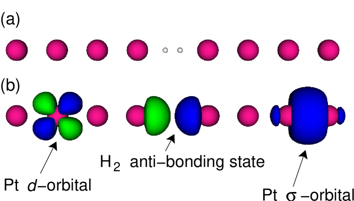
Figure 7: (a) Molecular hydrogen bridge connecting two semi-infinite, monatomic Pt chains. The atoms shown constitute the scattering region in the conductance calculation. (b) Contour plots of three representative basis functions. After diagonalizing the molecular subspace, the basis set consists of the initial WFs in the lead region and renormalized $\text{H}_{2}$ bonding and anti-bonding states in the molecular region.

In Fig. 8 we show the calculated transmission (thick line) as a function of energy. The transmission vanishes below $-6.5$ eV which marks the bottom of the $s$-band of the infinite Pt chain. The predicted conductance, $G=T(\varepsilon_{F})$, is found to be close to the experimental value of $1G_{0}$. Ideally, we would like to understand the shape of the transmission curve in terms of the properties of the uncoupled systems, i.e. the isolated $\text{H}_{2}$ molecule and the free leads. The interaction of a molecule with the leads can be seen as a two-step process: first the molecular levels are shifted (renormalized) due to the change in the potential from the leads. Next, the renormalized levels hybridize with the states in the leads as a consequence of the overlap between the wave functions. In the following we describe how the first step can be implemented and studied in practice. We will return to the second step in Sec. V.2.

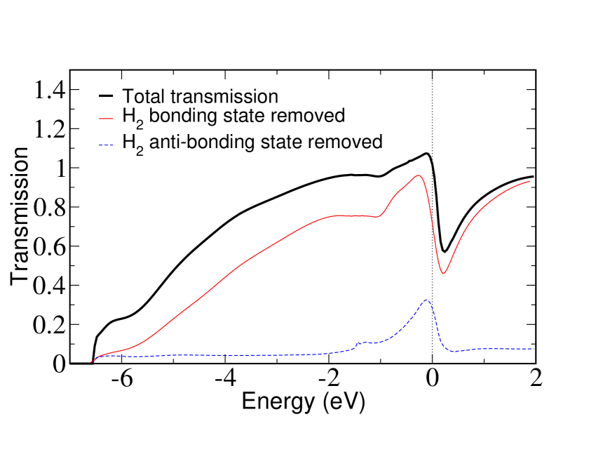
Figure 8: Transmission through the molecular hydrogen bridge shown in Fig. 7(a). The thick line represents the total transmission while the dashed and thin lines refer to the situations where the $\text{H}_{2}$ bonding, respectively anti-bonding states have been removed.

V.1.1 Diagonalization of the molecular subspace

In order to obtain the renormalized energy levels and orbitals of a molecule in contact with leads, we first construct the WFs for the combined system, i.e. the scattering region, and the corresponding Hamiltonian matrix, $\boldsymbol{H}_{S}$. Next, we identify the set of WFs located on the molecule. This involves some arbitrariness since it is not always clear where to put the separation between molecular WFs and lead WFs. Usually, the distinction is clearer when the bonding between molecule and lead is weaker. We refer to the space spanned by the molecular WFs as the molecular subspace. The renormalized molecular levels and orbitals are obtained by diagonalizing $\boldsymbol{H}_{S}$ within the molecular subspace. Since molecular orbitals to a large extent are determined by the symmetry of the molecule, it is usually straightforward to relate the renormalized orbitals to the orbitals of the free molecule. In contrast, the renormalized energies can be drastically shifted compared to the energies of the free molecule.

In the case of $\text{H}_{2}$ the molecular diagonalization produces a bonding, $|b\rangle$, and anti-bonding, $|a\rangle$, state from the initial $1s$-like WFs centered on each H. The renormalized energies are $\varepsilon_{b}=\langle b|H|b\rangle=-7.4$ eV and $\varepsilon_{a}=\langle a|H|a\rangle=0.4$ eV, relative to the Fermi level of the infinite chains. For comparison the corresponding energy levels of the free molecule before coupling are $-4.2$ eV and $6.6$ eV, respectively. The anti-bonding state is thus shifted down close to the Fermi level. This agrees with the conventional understanding of hydrogen dissociation on transition metal surfaces which has been established on the basis of DFT calculations hammer95 . In fact the filling of the $\text{H}_{2}$ anti-bonding state weakens the hydrogen bond and eventually leads to dissociation. The effect is less dramatic for hydrogen in the contact, however, the fractional filling of the anti-bonding state does enlarge the H-H bond length as compared to the free molecule. The reduction of the HOMO-LUMO gap from 10.8 eV in the free molecule to 7.8 eV in the contacted molecule is partly due to this structural effect ($\approx 1$ eV). The remaining reduction is due to the lead-induced change of the potential around the molecule. In Fig. 7(b) we show contour plots of $|a\rangle$ together with Pt $d$- and $\sigma$-like WFs.

Having obtained the renormalized molecular orbitals, it is natural to ask if there is significant interference between the two levels or if the conduction properties of the system are determined by just one of the two orbitals. A very direct way to answer this question, is to calculate the transmission with either the bonding or anti-bonding state removed. In practice this is done by setting all Hamiltonian matrix elements involving either $|b\rangle$ or $|a\rangle$ to zero. The resulting transmission curves are shown in Fig. 8. It is clear that the transmission is mainly due to the anti-bonding state and that interference effects are not very pronounced. The small peak in the transmission through the bonding state around the Fermi level is due to a peak at the same position in the DOS of the group orbital of $|b\rangle$ (see Sec. II.6). Although the use of monatomic chains as leads is an over-simplification, the main conclusions regarding the value of the conductance, the position of the molecular levels and the mechanism of conduction are unchanged when realistic bulk electrodes are used thygesen_h2 .

V.2 Benzene-dithiol between Au(111) surfaces

In this section we study the transmission through a benzene-dithiol molecule (BDT) suspended between Au(111) surfaces. The transport properties of this system have been investigated experimentally by Reed et al. reed97 using the mechanically controllable break junction technique, and several theoretical studies have been reported subsequently emberly01 ; diventra00 ; derosa01 ; stokbro03 ; xue_quantumchem . All of these studies are, like the present, based on a combination of the Landauer Büttiker formalism where a DFT description of the electronic structure enters at different levels. In general, the calculations for a BDT molecule covalently bonded to the electrodes finds a conductance which is 2-3 orders of magnitude higher than the experimental value. Different reasons for this discrepancy have been proposed including overlapping BDT molecules emberly01 and attachment of the BDT on top of a gold atom diventra00 . Here we focus on a symmetrically, covalently bonded molecule. We find a conductance comparable to those obtained in previous theoretical studies, however, we illustrate in addition how a proper construction of renormalized molecular orbitals leads to a very simple picture of the transport mechanism in terms of only two molecular states. The relatively large number of conductance calculations reported for the BDT system makes it an ideal test system for comparing different computation methods.

We use a supercell containing $3\times 3$ Au atoms in the directions perpendicular to the transport. The lead principal layer contains three atomic planes in accordance with the ABC-stacking. The scattering region contains 3 Au layers on each side of the DTB molecule which is enough to achieve a smooth matching with the bulk potential. To obtain a contact geometry which more closely resembles the open structures likely to occur in the experiments we insert a 3-atom pyramid between the surface and the molecule. The central part of the scattering region is shown in Fig. 9(a). We use the bond lengths $d_{\text{Au-S}}=2.40$ Å, $d_{\text{S-C}}=2.75$ Å, $d_{\text{C-C}}=1.40$ Å and $d_{\text{C-H}}=1.08$ Å in accordance with those used in Ref. stokbro03, . All gold atoms are fixed in an fcc lattice with lattice parameter $a=4.18$ Å.

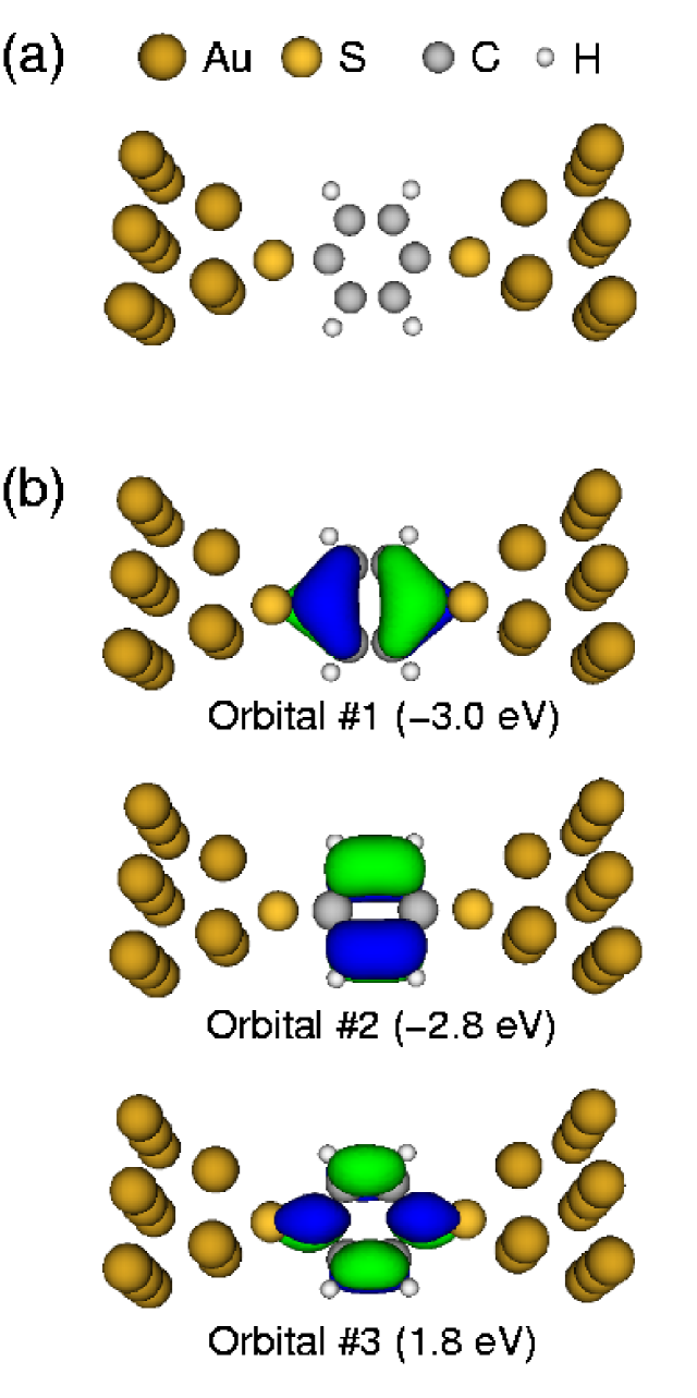
Figure 9: (a) Benzene-dithiol (BDT) between Au(111) surfaces. (b) The three renormalized molecular orbitals closest to the Fermi level of the electrodes. The renormalized energy is indicated in parenthesis. Orbital 2 (HOMO) has negligible weight on the S atoms and has no influence on the conduction properties. In contrast orbitals 1 and 3 are strongly coupled to the lead states and in fact they completely determine the transmission function.

In Fig. 10 we show the calculated transmission obtained using 1, 8 and 18 irreducible $\mathbb{k}$-points to sample the transverse BZ. The $\Gamma$-point transmission fluctuates very much compared to the converged result and is clearly not a good approximation. The rapid fluctuations are characteristic of $\Gamma$-point transmissions. This is because the lead in this case is simply a one-dimensional pipe with a $3\times 3$-atom cross section. The electronic structure of such relatively thin $1d$ structures is very different from the electronic structure of bulk systems, in particular the DOS of the former exhibits van Hove singularities at the $1d$ band edges thygesen_kpoints . We mention that the band dispersion between the free BDT molecules is less than 0.1 eV for all relevant orbitals. This shows that the $\mathbb{k}$-point dependence of the transmission function is not due to direct coupling between the repeated molecules, but is rather a substrate induced effect. The calculated transmission shows two broad peaks at around $-3.0$ eV and $2.5$ eV, and two more narrow peaks around $-1.5$ eV and $-1.0$ eV (all energies are with respect to the Fermi level of the leads). The occurrence of two broad peaks, one below and one above the Fermi level, is in qualitative agreement with previous results emberly01 ; stokbro03 ; xue_quantumchem . The position of these peaks as well as the existence of the two narrow peaks just below the Fermi level, are not in agreement with the earlier calculations which also deviate somewhat from each other. These discrepancies might be due to differences in the adopted geometries or technical issues like adequate $\mathbb{k}$-point sampling. In particular the result in Ref. emberly01, has been averaged over different atomic geometries which might smear out features related to details in the lead electronic structure. As we shall see, the narrow peaks arise exactly due to such details. Finally we note, that the predicted conductance is around $0.1G_{0}$. This is in very good agreement with the results obtained in Refs. emberly01, ; xue_quantumchem, , while it is a factor of 4 smaller than the result of Ref. stokbro03, and a factor of 3 larger than the result of Ref. diventra00, .

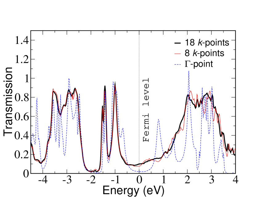
Figure 10: Calculated transmission through the bdt-system shown in Fig. 9 for three different $\mathbb{k}$-point samplings of the transverse BZ.

To investigate which orbitals of the BDT molecule are responsible for the different features of the transmission function we have performed a diagonalization of the molecular subspace as described in Sec. V.1.1. We define the molecular subspace as those WFs whose centers lie closer to the $\text{C}_{6}\text{H}_{4}$ molecule than to any other atom. The reason why we do not include the WFs at the S atoms in the molecular subspace is that S is three-fold coordinated to the gold and the ”weak” link in the contact is more naturally defined between S and C. Diagonalizing the Hamiltonian within the molecular subspace leads to 16 renormalized orbitals distributed in the energy range -17 eV to 5 eV. In Fig. 9(b) we show three renormalized molecular orbitals with energy close to the Fermi level. These orbitals all belong to the $\pi$-system of the molecule, i.e. they change sign under a reflection in the molecular plane.

Orbital 2 has negligible weight in the vicinity of the S atom and is expected to couple only weakly to the lead states. In contrast orbitals 1 and 3 have significant weight at the S-C bond and should therefore couple strongly with the leads and contribute correspondingly to the transmission. To obtain more quantitative information we have calculated the transmission function with all molecular orbitals except orbital 1, respectively 3, removed from the basis set, see Fig. 11. The result very clearly demonstrates that the broad peak at $-3$ eV is exclusively due to orbital 1, while the peak at $2.5$ eV is exclusively due to orbital 3. In particular interference between the different molecular orbitals does not occur around these energies. We can also conclude that the narrow peak at $-1.5$ eV is mostly due to orbital 3 while the narrow peak at $-1.0$ eV is mostly due to orbital 1, although the separation is not so clear in this case and interference effects do play a role.

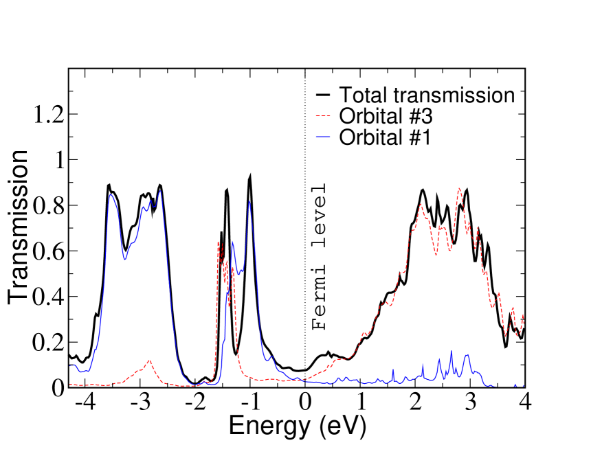
Figure 11: Calculated transmission through the bdt-system when all molecular orbitals except from orbital 1 (thin) and orbital 3 (dashed) have been removed. The total transmission (thick) is shown as a reference. All calculations have been performed using 8 irreducible $\mathbb{k}$-points. Notice, that the main transmission peak at $-3$ eV ($2$ eV) can be directly related to orbital 1 (3).

The above analysis shows that the transport properties of the BDT are completely determined by orbitals 1 and 3. To take the analysis even further we have constructed the corresponding group orbitals (see Sec. II.6), both of which are quite similar to an S-centered $p$-orbital perpendicular to the molecular plane. This is easily anticipated from the $\pi$ character of the molecular orbitals. According to Sec. II.6 the DOS of the group orbital calculated without coupling to the molecule, together with the level position and the coupling matrix element, determines the projected DOS for the corresponding molecular orbital. The group orbital DOS is shown in the upper panel of Fig. 12 (dashed line). We can model the DOS by a semi-elliptical band on top of a flat background (solid line), which allows us to compute the resulting DOS of an orbital with energy $\varepsilon_{a}$ and coupling $V$. The coupling can be directly extracted from the DFT Hamiltonian giving $V=1.3$ eV. Using the on-site energies of the renormalized orbitals 3 and 1, we obtain the DOS shown in the middle and bottom panel, respectively. In addition to the broad resonances formed close to the bare on-site energies, a narrow bonding, respectively anti-bonding resonance, involving the molecular orbital and the lead states, is formed at the edges of the semi-elliptical band. On the basis of these observations and the conductance formula Eq. (17) we can finally conclude that the transmission peaks at $2.5$ eV and $-1.5$ eV are due to orbital 3, while the peaks at $-3.0$ eV and $-1.0$ eV are due to orbital 1.

It is worth noting that the simplicity of the picture described above in terms of only two molecular orbitals relies on our definition of the molecular subspace. In Refs. stokbro03, ; derosa01, the transmission was analyzed in terms of the molecular orbitals of the whole BDT molecule stokbro03 , i.e. including the S atoms, and the BDT molecule plus selected Au atoms derosa01 . This leads to a more complicated description of the transmission peaks involving several different molecular orbitals. Thus the precise division of the Hilbert space into molecule- and lead-subspaces can lead to more or less elegant descriptions of transport properties.

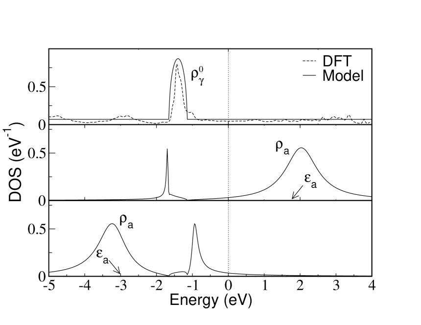
Figure 12: The upper panel shows the DOS, $\rho_{\gamma}^{0}$, of the (common) group orbital of molecular orbitals 1 and 3. $\rho_{\gamma}^{0}$ has been calculated with all coupling matrix elements involving the molecular orbitals set to 0, i.e. it refers to the uncoupled leads. The dashed line is the result obtained from the calculation, while the full line is a model fit. The two lower panels show the resulting DOS of a level

VI Conclusions

We have presented a numerical method for calculating electron transport in atomic-scale contacts. The method combines a formally exact Green’s function formalism with a mean-field description of the electronic structure based the Kohn-Sham scheme of density functional theory. By transforming the delocalized eigenstates obtained from an accurate plane-wave calculation, into maximally localized Wannier functions we obtain a highly efficient minimal basis set for evaluating the relevant Green’s functions. The construction scheme used to obtain the WFs has been introduced for both isolated and periodic systems and examples have been given to illustrate the important feature of bonding-antibonding closure. Finally, we have applied the transport scheme to a molecular hydrogen contact in a monatomic Pt wire and a benzene-dithiol molecule between Au(111) surfaces. A useful analysis technique for identifying which molecular orbitals contribute to which features of the transmission function has been introduced and applied to each of the systems. In this way we showed that the transport through the hydrogen molecule is determined by the anti-bonding state, and we identified two molecular orbitals which completely accounts for the transport through the benzene-dithiol.

VII Acknowledgments

We thank Lars B. Hansen for contributions to the Wannier function scheme. We acknowledge support from the Danish Center for Scientific Computing through Grant No. HDW-1101-05.

References

- (1) R. H. M. Smit, Y. Noat, C. Untiedt, N. D. Lang, M. C. van Hemert and J. M. van Ruitenbeek, Nature 419, 906 (2002).
- (2) M. A. Reed, C. Zhou, C. J. Muller, T. P. Burgin and J. M. Tour, Science 278, 252 (1997).
- (3) S. Datta, Electronic Transport in Mesoscopic Systems Cambridge Univ. Press, (1997).
- (4) Y. Imry, Introduction to Mesoscopic Physics Oxford Univ. Press, (1997).
- (5) N. Agrait, A. L. Yeyati and J. M. van Ruitenbeek, Physics Reports, 377, 81-279 (2003).
- (6) M. Büttiker, Y. Imry, R. Landauer and S. Pinhas, Phys. Rev. B, 31, 6207 (1985).
- (7) P. Sautet and C. Joachim, Phys. Rev. B, 38, 12238 (1988).
- (8) E. G. Emberly and G. Kirczenow, Phys. Rev. B, 58, 10911 (1998).
- (9) H. J. Choi and J. Ihm, Phys. Rev. B, 59, 2267 (1999).
- (10) K. Hirose and M. Tsukada, Phys. Rev. Lett., 73, 150 (1994).
- (11) K. Hirose and M. Tsukada, Phys. Rev. B, 51, 5278 (1995).
- (12) N. Kobayashi, M. Brandbyge and M. Tsukada, Phys. Rev. B, 62, 8430 (2000).
- (13) P. A. Khomyakova and G. Brocks, arXiv:cond-mat/0405151, (2004).
- (14) N. D. Lang, Phys. Rev. B, 52, 5335 (1995).
- (15) M. Di Ventra, S. T. Pantelides and N. D. Lang, Phys. Rev. Lett. 84, 979 (2000).
- (16) L. V. Keldysh, Soviet Physics JETP-USSR, 20:1018 (1965).
- (17) L. P. Kadanoff and G. Baym, Quantum Statistical Mechanics, Benjamin (1962).
- (18) T. Frederiksen, M. Brandbyge, N. Lorente and A. P. Jauho arXiv:cond-mat/0410700, (2004).
- (19) Y. Meir and N. S. Wingreen, Phys. Rev. Lett. 68, 2512 (1992).
- (20) M. B. Nardelli, Phys. Rev. B 60, 7828 (1999).
- (21) A. L. Yeyati, A. Martín-Rodero and F. Flores Phys. Rev. B 56, 10369 (1997).
- (22) J. Taylor, H. Guo and J. Wang, Phys. Rev. B, 63, 245407 (2001).
- (23) Y. Xue, S. Datta and M. A. Ratner, Chem. Phys.,281, 151 (2001).
- (24) M. Brandbyge, J. L. Mozos, P. Ordejón, J. Taylor and K. Stokbro Phys. Rev. B 65, 165401 (2002).
- (25) K. S. Thygesen, M. V. Bollinger and K. W. Jacobsen, Phys. Rev. B 67, 115404 (2003).
- (26) A. Calzolari, N. Marzari, I. Souza, M. B. Nardelli, Phys. Rev. B 69, 035108 (2004).
- (27) San-Huang Ke, Harold U. Baranger, and Weitao Yang, Phys. Rev. B 70, 085410 (2004).
- (28) J. Heurich, J. C. Cuevas, W. Wenzel and G. Schön, Phys. Rev. Lett. 88, 256803 (2002).
- (29) P. A. Derosa and J. M. Seminario, J. Phys. Chem. B 105, 471 (2001).
- (30) J. J. Palacios, A. J. Pérez-Jiménez, E. Louis and J. A. Vergés Phys. Rev. B 64, 115411 (2001).
- (31) F. Guinea, C. Tejedor, F. Flores and E. Louis, Phys. Rev. B,28, 4397 (1983).
- (32) G. B. Bachelet, D. R. Hamann and M. Schlüter, Phys. Rev. B,26, 4199 (1982).
- (33) D. R. Hamann, M. Schlüter and C. Chiang Phys. Rev. Lett.,43, 1494 (1979).
- (34) D. Vanderbilt, Phys. Rev. B 41, 7892 (1990).
- (35) D. M. Newns, Phys. Rev. 178, 1123 (1969).
- (36) K. S. Thygesen and K. W. Jacobsen, arXiv:cond-mat/0411086, Phys. Rev. Lett. accepted.
- (37) I. Souza, N. Marzari and D. Vanderbilt, Phys. Rev. B 65, 035109 (2001).
- (38) M. Iannuzzi and M. Parrinello, Phys. Rev. B 66, 155209 (2002).
- (39) N. Marzari and D. Vanderbilt, Phys. Rev. B 56, 12847 (1997).
- (40) R. Resta and S. Sorella, Phys. Rev. Lett. 82, 370 (1999).
- (41) G. Berghold, C. J. Mundy, A. H. Romero, J. Hutter and M. Parrinello, Phys. Rev. B 61, 10040 (2000).
- (42) P. L. Silvestrelli, N. Marzari, D. Vanderbilt and M. Parrinello, Solid State Commun. 107, 7 (1998).
- (43) J. C. Cuevas, J. Heurich, F. Pauly, W. Wenzel, and G. Schön, Nanotechnology, 14, R29 (2003).
- (44) K. S. Thygesen and K. W. Jacobsen, arXiv:cond-mat/0411088, Phys. Rev. Lett. accepted.
- (45) Y. García, J. J. Palacios, E. SanFabián, J. A. Vergés, A. J. Pérez-Jiménez and E. Louis, Phys. Rev. B 69, 041402(R) (2004).
- (46) B. Hammer and J. K. Nørskov, Surface Science 343, 211 (1995).
- (47) E. G. Emberly and G. Kirczenow, Phys. Rev. B 64, 235412 (2001).
- (48) K. Stokbro, J. Taylor, M. Brandbyge, J. -L. Mozos and P. Ordejón, Comp. Matt. Science 27, 151 (2003).
- (49) Y. Xue, M. A. Ratner arXiv:cond-mat/0401539.
- (50) K. S. Thygesen and K. W. Jacobsen, arXiv:cond-mat/0411589.