Dynamics of Shuttle Devices

Andrea Donarini

Ph.D. Thesis

Technical University of Denmark

phd

Foreword

This thesis is submitted in candidacy for the Ph.D. degree within the Physics Program at the Technical University of Denmark. The thesis describes part of the work that I have carried out under supervision of Antti-Pekka Jauho from the Department of Micro and Nanotechnology.

I’m grateful to my supervisor for the very stimulating atmosphere that he has been able to create and maintain within his group and also for his gentle but firm guidance. I want to thank all the members of the Theoretical Nanotechnology Group at the MIC Department and in particular Dr. Tomáš Novotný and Christian Flindt for the close and intense collaboration that has generated a large part of the results presented in this thesis.

I would like to thank Prof. Timo Eirola for having introduced me to the subject of the iterative numerical methods and for his precious help in the solution of some of the numerical problems I encounter in my research. I want also to thank Dr. Tobias Brandes and Neill Lambert for the nice physics discussions I could have with them during the period I spent collaborating with them in Manchester. I want to thank Christian Flindt also for the enthusiasm and the very positive attitude that he has been always able to spread within the “Shuttle Group”. He has also been an indefatigable reader of the proofs and deserves many thanks for that. Finally I also want to thank my family for their far but constant support and all the Italian friends in Copenhagen for being very patient and encouraging me during the writing period.

Lyngby, September 3, 2004

Andrea Donarini

phd

Preface

Much interest has been drawn in recent years to the concept and realization of Nanoelectromechanical systems (NEMS). NEMS are nanoscale devices that combine mechanical and electrical dynamics in a strong interplay. The shuttle devices are a particular kind of Nanoelectromechanical systems. The characteristic component that gives the name to these devices is an oscillating quantum dot of nanometer size that transfers electrons one-by-one between a source and a drain lead. The device represents the nano-scale analog of an electromechanical bell in which a metallic ball placed between the plates of a capacitor starts to oscillate when a high voltage is applied to the plates.

This thesis contains the description and analysis of the dynamics of two realizations of quantum shuttle devices. We describe the dynamics using the Generalized Master Equation approach: a well-suited method to treat this kind of open quantum systems. We also classify the operating modes in three different regimes: the tunneling, the shuttling and the coexistence regime. The characterization of these regimes is given in terms of three investigation tools: Wigner distribution functions, current and current-noise. The essential dynamics of these regimes is captured by three simplified models whose derivation from the full description is possible due to the time scale separation of the particular regime. We also obtain from these simplified models a more intuitive picture of the variety of different dynamics exhibited by the shuttle devices.

Lyngby, October 10, 2004

Andrea Donarini

phd

Chapter 1 Introduction

In this chapter we give a short introduction to the world of nanoelectromechanical systems. We then focus our attention on a particular kind of device called electron shuttle. We sketch the basic operating regime and give an overview of the different theoretical models that have been proposed to describe the dynamics of such devices. We report on the two main realizations of shuttle devices and close the chapter with an outline of the contents of this thesis.

1.1 NEMS

Much interest has been drawn in recent years on the concepts and realization of Nanoelectromechanical systems (NEMS). NEMS are nanoscale devices that combine mechanical and electrical dynamics in a strong interplay. This property makes them interesting both from a technological and fundamental point of view. They are extremely sensitive mass and position detectors. Due to their very high mechanical frequency one can even think of using them as the basis for new form of mechanical computers. From the point of view of fundamental research they represent extremely good tools to probe directly the basic quantum mechanical laws. They could represent the first man-made structures on which the mechanical zero point fluctuation can be detected. They also rise the question on the limiting dimension for persistence of mechanical coherence. In general one of the fascinating aspects of these objects is their mesoscopic character: they share with the macroscopic world the large number of atoms of which they are made (typically of millions of atoms) but on the other hand their behaviour is (or should be) already significantly determined by quantum mechanics.

1.2 A new transport regime

The shuttle devices are a particular kind of NEMS. The characteristic component that gives the name to these devices is an oscillating object of nanometer size that transfers electrons one-by-one between a source and a drain lead. The device represents the nano-scale analog of an electromechanical bell in which a metallic ball placed between the plates of a capacitor starts to oscillate when a high voltage is applied to the plates. The oscillations are sustained by the external bias that pumps energy into the mechanical system: when the ball is in contact with the negatively biased plate it gets charged and the electrostatic field drives it towards the other capacitor plate where the ball releases the electrons and returns back due to the oscillator restoring forces111Due to the large amount of electrons in this macroscopic realization the ball gets positively charged at the second plate by loosing some extra electrons and the restoring force contains also an electrostatic component. The system is perfectly symmetric under commutation of charge sign. and the cycle starts again.

In the first proposal [1] of a shuttle device the movable carrier is a metallic grain confined into a harmonic potential by elastically deformable organic molecular links attached to the leads. The transfer of charge is governed by tunneling events, the tunneling amplitude being modulated by the position of the oscillating grain. The exponential dependence of the tunneling amplitude of the grain position leads to an alternating opening and closing of the left and right tunneling channels that resembles the charging and discharging dynamics of the macroscopic analog.

Different models for shuttle devices have been proposed in the literature since this first seminal work by Gorelik et al. [1]. The mechanical degree of freedom has been treated classically (using harmonic [2, 3, 4, 5] or more realistic potentials [6]) and quantum mechanically [7, 8, 9]. Armour and MacKinnon proposed a model with the oscillating grain flanked by two static quantum dots [7, 10, 11, 12]. More generally the shuttling mechanism has been applied to Cooper pair transport [13, 14] and pumping of superconducting phase [15] or magnetic polarization [16].

The essential feature of the nano-scale realization is the quantity transferred per cycle (a charge up to 1010superscript101010^{10} electrons for a macroscopic bell) that is scaled down to 1 quantum unit (electron, spin, Cooper pair in the different realizations). We can already guess the basic properties of the shuttle transport:

  1. 1.

    Charge-position correlation: the shuttling dot loads the charge on one side and transfers it on the other side, it releases it and returns back to the starting point;

  2. 2.

    Matching between electronic and mechanical characteristic times (non-adiabaticity);

  3. 3.

    Quantized current determined by the mechanical frequency;

  4. 4.

    Low current fluctuations: the stochasticity of the tunneling event is suppressed due to an interplay between mechanical and electrical properties. The tunneling event is only probable at some particular short time periods fixed by the mechanical dynamics (i.e. when the oscillating dot is close to a specific lead).

1.3 Experimental implementations

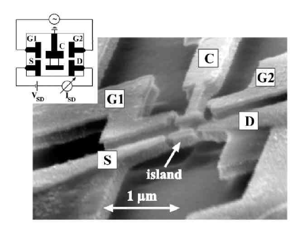
An experimental realization of the shuttle device has been produced by Erbe et al. [17]. The structure consists of a cantilever with a quantum island at the top placed between source and drain leads. Two lateral gates can set the cantilever into motion via a capacitive coupling. An ac voltage applied at these gates makes the cantilever vibrating and brings the tip alternatively closer to the source or drain lead and thus allows the shuttling of electrons.
Refer to caption
Figure 1.1: Electron micrograph of the nano-mechanical resonator. The cantilever (C) can be set into motion by applying an ac-voltage between the two gates G1 and G2, and by applying a bias across the metallic tip of the cantilever (the island) electrons are shuttled from the source (S) to the drain (D). The picture is taken from [17].

The device (shown in Fig. 1.1) is built out of silicon-on-insulator (SOI) materials (using Au for the metallic parts) using etch mask techniques and optical and electron beam lithography. The cantilever is 1μm1𝜇𝑚~{}1\mu m long and the corresponding resonant frequency is of the order of 100MHz100MHz100{\,\rm MHz}. The source electrode and the cantilever are at an average distance of approximately 0.1μm0.1𝜇𝑚0.1\,\mu m. Shuttling experiments have been performed by Erbe et al. at different temperatures. For experiments at 4.2K4.2K4.2\,{\rm K} and 12K12K12\,{\rm K} they measured a pronounced peak in the current through the cantilever for a driving frequency of approximately 120MHz120MHz120\,{\rm MHz} corresponding to the natural frequency of the first mode of the oscillator. The peak in the current corresponds to a rate of shuttle success of about one electron per 9 mechanical cycles. The Erbe experiment is very close to the original proposal by Gorelik. The only difference is in the external driving of the mechanical oscillations. In the original proposal the bias was time independent and the driving induced by the electrostatic force on the charged oscillating island. The initially stochastic tunneling events would eventually cause the shuttling instability and drive the system into a self-sustained mechanical oscillation combined with periodic charging and discharging events.
Refer to caption
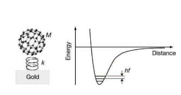
Figure 1.2: The C60 experiment by Park et al. The C60 molecule (of mass M) can be considered as being attached to a spring with spring constant k𝑘k and corresponding quantized excitation energy hf𝑓hf of the order of 5 meV. The figure is taken from [18].

Another experiment often mentioned in the context of quantum shuttles is the C60-experiment by Park et al. [18] In this experiment a C60 molecule is deposited in the gap between two gold electrodes. The gap, produced with break junction technique, has a width of 1 nm. The molecule (of diameter 0.7 nm) is bound to the electrodes due to van der Waals interaction. Around the equilibrium position the potential can be approximated by a harmonic potential and the molecule can be considered as attached by springs. We show a schematic representation of this idea in Fig. 1.2. In the experiment Park et al. sweep the voltage across the junction and register sudden increases in the current. The steps are separated by 5 meV. Since the lowest internal excitation energy of the C60 molecule is 353535 meV one concludes that the slower center of mass motion could be involved in the process. This hypothesis is confirmed by the fact that the separation between the steps is independent of the charge on the C60 molecule and the theoretical estimate for the energy corresponding to the center of mass oscillation in the van der Waals potential is exactly 5 meV. The IV-curve measured in these experiments can be interpreted in terms of shuttling [19], but also alternative explanations have been promoted [20, 21, 22]. Whether we are in presence of coherent or incoherent shuttling transport and to what extent the shuttling mechanism is involved in this set-up cannot be completely clarified by current measurement. The current-current correlation (also called current noise) was proposed by Fedorets et al. [19] for a better understanding of the underlying dynamics of the current jumps. For this reason the calculation of noise in shuttle devices has been performed by many different groups. We proposed a completely quantum formulation [23] that is also explained in detail in this thesis.

1.4 This thesis

This thesis contains the description and analysis of the dynamics of two realizations of quantum shuttle devices. The models we consider describe both the mechanical and electrical degrees of freedom quantum mechanically. For the single dot quantum shuttle we extended an existing classical model proposed by Gorelik et al. [1]. For the triple dot case we adopted the model invented by Armour and MacKinnon [7]. In the following we outline the contents of the thesis:

In Chapter 2 we introduce the two models called Single Dot Quantum Shuttle and Triple Dot Quantum Shuttle, the first being the quantum extension also for the mechanical degree of freedom of the model originally proposed by Gorelik et al. [1] while the second is the model invented by Armour and MacKinnon [7]. Also in this model the oscillator is treated quantum mechanically and the central moving dot is flanked by two static dots.

We dedicate Chapter 3 to the derivation of the Generalized Master Equation (GME) that describes the shuttle device dynamics. Due to the different coupling strengths we treat the mechanical and electrical baths with two different approaches. The Gurvitz approach for the electrical and the standard Born-Markov approximation for the mechanical bath. The derivation à la Gurvitz represents a large part of this chapter. In order to facilitate the understanding of this non-standard method and appreciate our extension to the shuttle device we have given a long introduction in which we analyze in great detail simpler models with increasing physical complexity. This shows on one hand the essence of the derivation in simpler cases and also underlines the potentiality of this approach. An important aspect of this method is also to be a natural prelude to full counting statistics since it naturally produces a GME that counts the number of electron which tunneled through the device at a certain time. We close the chapter with the description of the numerical iterative method that we adopted for the calculation of the stationary solution of the GME.

In Chapter 4 we introduce the concept of Wigner distribution function and derive the corresponding Klein-Kramers equation for the SDQS starting from the GME that we obtained in the previous chapter. The Wigner function description is motivated by the effort to keep the complete quantum treatment we achieved with the GME without losing as much as possible the intuitive classical picture and with the possibility to handle the quantum-classical correspondence.

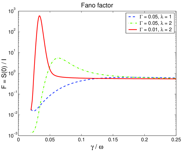
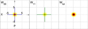
Chapter 5 is dedicated to the definition and application of the three investigation tools we have chosen to analyze the properties of shuttle devices: the charge resolved phase-space distribution, the current and the current-noise. The phase space analysis reveals the shuttling transition and the charge position correlation typical of this operating regime. It also gives a very clean way to appreciate “geometrically” the quantum to classical transition of the shuttling behaviour for different device realizations. The second investigation tool that we consider is the current. From the current calculation we obtain also in the quantum treatment the quantized value of one electron per cycle found in the semiclassical treatments of similar devices. We then present current-noise calculations based on the MacDonald formula. The derivation is strongly dependent on the derivation à la Gurvitz of the n𝑛n-resolved GME. The low noise quasi-deterministic behaviour of the shuttling transport is clear from the extremely low Fano factors found for this regime. In general we are able with all the three investigation tools to identify three operating regimes of shuttle devices: the tunneling, shuttling and coexistence regimes.

Chapter 6 is dedicated to a qualitative description of the these regimes and also to the identification of the relation between different times and length scales that define the three regimes in terms of the model parameters.

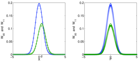
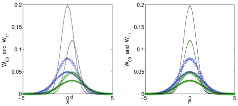
In Chapter 7 we consider separately the tunneling, shuttling and coexistence regime. The specific separation of time scales allows us to identify the relevant variables and describe each regime by a specific simplified model. Models for the tunneling, shuttling and coexistence regime are analyzed in this chapter. We also give a comparison with the full description in terms of Wigner distributions, current and current-noise to prove that the models, at least in the limits set by the chosen investigation tools, capture the relevant dynamics.

A summary of the arguments treated in this thesis opens Chapter 8. We conclude with a list of some of the open questions that could encourage a continuation of the present work.

Chapter 2 The models

We describe in this chapter two models of quantum shuttles: the Single-Dot Quantum Shuttle and the Triple-Dot Quantum Shuttle. Due to the nanometer size of these devices we decide to treat quantum mechanically not only the electrical but also the mechanical dynamics. This approach was suggested by the work of Armour and MacKinnon [7] for the triple dot device and implemented for the first time by us in the single dot device.

2.1 Single-Dot Quantum Shuttle

The Single-Dot Quantum Shuttle (SDQS) consists of a movable quantum dot (QD) suspended between source and drain leads. One can imagine the dot attached to the tip of a cantilever or connected to the leads by some soft legands or embedded into an elastic matrix. In the model the center of mass of the nanoparticle is confined to a potential that, at least for small diplacements from its equilibrium position, can be considered harmonic. We give a schematic visualization of the device in figure 2.1.

Refer to caption
Figure 2.1: Schematic representation of the Single-dot Shuttle: electrons tunnel from the left lead at chemical potential (μLsubscript𝜇𝐿\mu_{L}) to the quantum dot and eventually to the right lead at lower chemical potential μRsubscript𝜇𝑅\mu_{R}. The position dependent tunneling amplitudes are indicated. X𝑋X is the displacement from the equilibrium position. The springs represent the harmonic potential in which the central dot can move.

Due to its small diameter, the QD has a very small capacitance and thus a charging energy that exceeds (in the most recent realizations almost at room temperature [24]) the thermal energy kBTsubscript𝑘𝐵𝑇k_{B}T111A quick estimate of the charging energy can be obtained for an isolated 2D metallic disk: e2/C=e2/(8ϵrϵ0R)superscript𝑒2𝐶superscript𝑒28subscriptitalic-ϵ𝑟subscriptitalic-ϵ0𝑅e^{2}/C=e^{2}/(8\epsilon_{r}\epsilon_{0}R) where R is the disk radius and ϵr=13subscriptitalic-ϵ𝑟13\epsilon_{r}=13 in GaAs. For a dot of radius 10 nm this yields e2/C=20meV=kB230Ksuperscript𝑒2𝐶20meVsubscript𝑘𝐵230Ke^{2}/C=20{\rm meV}=k_{B}230{\rm K} . For this reason we assume that only one excess electron can occupy the device (Coulomb blockade) and we describe the electronic state of the central dot as a two-level system (empty/charged). Electrons can tunnel between leads and dot with tunneling amplitudes which are exponentially dependent on the position of the central island. This is due to the exponentially decreasing/increasing overlapping of the electronic wave functions.

The Hamiltonian of the model reads:

H=Hsys+Hleads+Hbath+Htun+Hint𝐻subscript𝐻syssubscript𝐻leadssubscript𝐻bathsubscript𝐻tunsubscript𝐻intH=H_{\rm sys}+H_{\rm leads}+H_{\rm bath}+H_{\rm tun}+H_{\rm int} (2.1)

where

Hsys=p^22m+12mω2x^2+(ε1ex^)c1c1Hleads=k(εlkclkclk+εrkcrkcrk)Htun=k[Tl(x^)clkc1+Tr(x^)crkc1]+h.c.Hbath+Hint=genericheatbathformulae-sequencesubscript𝐻syssuperscript^𝑝22𝑚12𝑚superscript𝜔2superscript^𝑥2subscript𝜀1𝑒^𝑥superscriptsubscript𝑐1superscriptsubscript𝑐1absentsubscript𝐻leadssubscript𝑘subscript𝜀subscript𝑙𝑘subscriptsuperscript𝑐subscript𝑙𝑘subscriptsuperscript𝑐absentsubscript𝑙𝑘subscript𝜀subscript𝑟𝑘subscriptsuperscript𝑐subscript𝑟𝑘subscriptsuperscript𝑐absentsubscript𝑟𝑘subscript𝐻tunsubscript𝑘delimited-[]subscript𝑇𝑙^𝑥subscriptsuperscript𝑐subscript𝑙𝑘superscriptsubscript𝑐1absentsubscript𝑇𝑟^𝑥subscriptsuperscript𝑐subscript𝑟𝑘superscriptsubscript𝑐1absent𝑐subscript𝐻bathsubscript𝐻intgenericheatbath\begin{split}&H_{\rm sys}=\frac{\hat{p}^{2}}{2m}+\frac{1}{2}m\omega^{2}\hat{x}^{2}+(\varepsilon_{1}-e\mathcal{E}\hat{x})c_{1}^{{\dagger}}c_{1}^{\phantom{\dagger}}\\ &H_{\rm leads}=\sum_{k}(\varepsilon_{l_{k}}c^{\dagger}_{l_{k}}c^{\phantom{\dagger}}_{l_{k}}+\varepsilon_{r_{k}}c^{\dagger}_{r_{k}}c^{\phantom{\dagger}}_{r_{k}})\\ &H_{\rm tun}=\sum_{k}[T_{l}(\hat{x})c^{\dagger}_{l_{k}}c_{1}^{\phantom{\dagger}}+T_{r}(\hat{x})c^{\dagger}_{r_{k}}c_{1}^{\phantom{\dagger}}]+h.c.\\ &H_{\rm bath}+H_{\rm int}={\rm generic\;heat\;bath}\end{split} (2.2)

Using the language of quantum optics we call the movable grain alone the system. This is then coupled to two electric baths (the leads) and a generic heat bath. The system is described by a single electronic level of energy ε1subscript𝜀1\varepsilon_{1} and a harmonic oscillator of mass m𝑚m and frequency ω𝜔\omega. When the dot is charged the electrostatic force (e𝑒e\mathcal{E}) acts on the grain and gives the electrical influence on the mechanical dynamics. The electric field \mathcal{E} is generated by the voltage drop between left and right lead. In our model, though, it is kept as an external parameter, also in view of the fact that we will always assume the potential drop to be much larger than any other energy scale of the system (with the only exception of the charging energy of the dot). The operator form x^,p^^𝑥^𝑝\hat{x},\hat{p} for the mechanical variables is due to the quantum treatment of the harmonic oscillator. In terms of creation and annihilation operators for oscillator excitations we would write:

x^=2mω(d+d)p^=imω2(dd)p^22m+12mω2x^2=ω(dd+12)^𝑥Planck-constant-over-2-pi2𝑚𝜔superscript𝑑𝑑^𝑝𝑖Planck-constant-over-2-pi𝑚𝜔2superscript𝑑𝑑superscript^𝑝22𝑚12𝑚superscript𝜔2superscript^𝑥2Planck-constant-over-2-pi𝜔superscript𝑑𝑑12\begin{split}&\hat{x}=\sqrt{\frac{\hbar}{2m\omega}}(d^{\dagger}+d)\\ &\hat{p}=i\sqrt{\frac{\hbar m\omega}{2}}(d^{\dagger}-d)\\ &\frac{\hat{p}^{2}}{2m}+\frac{1}{2}m\omega^{2}\hat{x}^{2}=\hbar\omega\left(d^{\dagger}d+\frac{1}{2}\right)\end{split} (2.3)

The leads are Fermi seas kept at two different chemical potentials (μLsubscript𝜇𝐿\mu_{L} and μRsubscript𝜇𝑅\mu_{R}) by the external applied voltage (ΔV=(μLμR)/eΔ𝑉subscript𝜇𝐿subscript𝜇𝑅𝑒\Delta V=(\mu_{L}-\mu_{R})/e ). The oscillator is immersed into a dissipative environment that we model as a collection of bosons and is coupled to that by a weak bilinear interaction:

Hbath=𝐪ω𝐪d𝐪d𝐪Hint=𝐪g(d𝐪+d𝐪)(d+d)subscript𝐻bathsubscript𝐪Planck-constant-over-2-pisubscript𝜔𝐪superscriptsubscript𝑑𝐪subscript𝑑𝐪subscript𝐻intsubscript𝐪Planck-constant-over-2-pi𝑔subscript𝑑𝐪superscriptsubscript𝑑𝐪𝑑superscript𝑑\begin{split}H_{\rm bath}&=\sum_{\mathbf{q}}\hbar\omega_{\mathbf{q}}{d_{\mathbf{q}}}^{\dagger}d_{\mathbf{q}}\\ H_{\rm int}&=\sum_{\mathbf{q}}\hbar g({d_{\mathbf{q}}}+{d_{\mathbf{q}}}^{\dagger})(d+d^{\dagger})\end{split} (2.4)

where the bosons have been labelled by their wave number 𝐪𝐪\mathbf{q}. The damping rate is given by:

γ(ω)=2πg2D(ω)𝛾𝜔2𝜋superscript𝑔2𝐷𝜔\gamma(\omega)=2\pi g^{2}D(\omega) (2.5)

where D(ω)𝐷𝜔D(\omega) is the density of states for the bosonic bath at the frequency of the system oscillator. A bath that generates a frequency independent γ𝛾\gamma is called Ohmic.

The coupling to the electric baths is introduced by the tunneling Hamiltonian Htunsubscript𝐻tunH_{\rm tun}. The tunneling amplitudes Tl(x^)subscript𝑇𝑙^𝑥T_{l}(\hat{x}) and Tr(x^)subscript𝑇𝑟^𝑥T_{r}(\hat{x}) depend exponentially on the position operator x^^𝑥\hat{x} and represent the mechanical feedback on the electrical dynamics:

Tl,r(x^)=tl,rexp(x^/λ)subscript𝑇𝑙𝑟^𝑥subscript𝑡𝑙𝑟minus-or-plus^𝑥𝜆T_{l,r}(\hat{x})=t_{l,r}\exp(\mp\hat{x}/\lambda) (2.6)

where λ𝜆\lambda is the tunneling length. The tunneling rates from and to the leads (Γ¯L,Rsubscript¯Γ𝐿𝑅\bar{\Gamma}_{L,R}) can be expressed in terms of the amplitudes:

Γ¯L,R=ΓL,R(x^)=2πDL,Rexp(2x^λ)|tl,r|2subscript¯Γ𝐿𝑅delimited-⟨⟩subscriptΓ𝐿𝑅^𝑥delimited-⟨⟩2𝜋Planck-constant-over-2-pisubscript𝐷𝐿𝑅minus-or-plus2^𝑥𝜆superscriptsubscript𝑡𝑙𝑟2\bar{\Gamma}_{L,R}=\langle\Gamma_{L,R}(\hat{x})\rangle=\left\langle\frac{2\pi}{\hbar}D_{L,R}\exp\left(\mp\frac{2\hat{x}}{\lambda}\right)|t_{l,r}|^{2}\right\rangle (2.7)

where DL,Rsubscript𝐷𝐿𝑅D_{L,R} are the densities of states of the left and right lead respectively and the average is taken with respect to the quantum state of the oscillator.

The model presents three relevant time scales: the period of the oscillator 2π/ω2𝜋𝜔2\pi/\omega, the inverse of the damping rate 1/γ1𝛾1/\gamma and the average injection/ejection time 1/Γ¯L,R1subscript¯Γ𝐿𝑅1/\bar{\Gamma}_{L,R}. It is possible also to identify three important length scales: the zero point uncertainty Δxz=2mωΔsubscript𝑥𝑧Planck-constant-over-2-pi2𝑚𝜔\Delta x_{z}=\sqrt{\frac{\hbar}{2m\omega}}, the tunneling length λ𝜆\lambda and the displaced oscillator equilibrium position d=emω2𝑑𝑒𝑚superscript𝜔2d=\frac{e\mathcal{E}}{m\omega^{2}}. Different relations between time and length scales distinguish different operating regimes of the SDQS.

2.2 Triple-Dot Quantum Shuttle

The Triple-Dot Quantum Shuttle (TDQS) was proposed by Armour and MacKinnon [7]. The system consists of an array of three QD’s: a movable dot, that we assume confined to a harmonic potential, flanked by two static ones. Relying on low temperature and on the low capacitance of the system with respect to the leads, we again assume strong Coulomb blockade: only one electron at a time can occupy the three-dot device. The Hamiltonian for the model reads:

H=Hsys+Hleads+Hbath+Htun+Hint𝐻subscript𝐻syssubscript𝐻leadssubscript𝐻bathsubscript𝐻tunsubscript𝐻intH=H_{\rm sys}+H_{\rm leads}+H_{\rm bath}+H_{\rm tun}+H_{\rm int} (2.8)

Only the system and tunneling part of the Hamiltonian differ from the one dot case:

Hsys=ϵ0|00|+ΔV2|LL|ΔV2x0x^|CC|ΔV2|RR|+ω(dd+12)+tR(x^)(|CR|+|RC|)+tL(x^)(|CL|+|LC|)Htun=kTl(clk|0L|+clk|L0|)+Tr(crk|0R|+crk|R0|)subscript𝐻syssubscriptitalic-ϵ0ket0quantum-operator-product0Δ𝑉2𝐿quantum-operator-product𝐿Δ𝑉2subscript𝑥0^𝑥𝐶quantum-operator-product𝐶Δ𝑉2𝑅bra𝑅Planck-constant-over-2-pi𝜔superscript𝑑𝑑12subscript𝑡𝑅^𝑥ket𝐶bra𝑅ket𝑅bra𝐶subscript𝑡𝐿^𝑥ket𝐶bra𝐿ket𝐿bra𝐶subscript𝐻tunsubscript𝑘subscript𝑇𝑙subscriptsuperscript𝑐subscript𝑙𝑘ket0quantum-operator-product𝐿subscriptsuperscript𝑐absentsubscript𝑙𝑘𝐿bra0subscript𝑇𝑟subscriptsuperscript𝑐subscript𝑟𝑘ket0quantum-operator-product𝑅subscriptsuperscript𝑐absentsubscript𝑟𝑘𝑅bra0\begin{split}H_{\rm sys}=&\epsilon_{0}|0\rangle\!\langle 0|+\frac{\Delta V}{2}|L\rangle\!\langle L|-\frac{\Delta V}{2x_{0}}\hat{x}|C\rangle\!\langle C|-\frac{\Delta V}{2}|R\rangle\!\langle R|+\hbar\omega\left(d^{{\dagger}}d+\frac{1}{2}\right)\\ &+t_{R}(\hat{x})(|C\rangle\!\langle R|+|R\rangle\!\langle C|)+t_{L}(\hat{x})(|C\rangle\!\langle L|+|L\rangle\!\langle C|)\\ H_{\rm tun}=&\sum_{k}T_{l}(c^{\dagger}_{l_{k}}|0\rangle\!\langle L|+c^{\phantom{\dagger}}_{l_{k}}|L\rangle\!\langle 0|)+T_{r}(c^{\dagger}_{r_{k}}|0\rangle\!\langle R|+c^{\phantom{\dagger}}_{r_{k}}|R\rangle\!\langle 0|)\end{split} (2.9)

where Hoscsubscript𝐻oscH_{\rm osc} is the harmonic-oscillator Hamiltonian, |α,α=0,L,C,Rformulae-sequenceket𝛼𝛼0𝐿𝐶𝑅|\alpha\rangle,\alpha=0,L,C,R are the vectors that span the electronic part of the system Hilbert space . The tunable injection and ejection energies (the energy levels of the outer dots, that we can assume fixed by external gates) simulate a controlled bias through the device (ΔVΔ𝑉\Delta V) and the position dependent tunneling amplitudes are now between elements within the system. These amplitude are assumed to be exponentially dependent on the position of the central dot tL(x^)=V0e(x0+x^)/λsubscript𝑡𝐿^𝑥subscript𝑉0superscript𝑒subscript𝑥0^𝑥𝜆t_{L}(\hat{x})=-V_{0}e^{-(x_{0}+\hat{x})/\lambda} and tR(x^)=V0e(x0x^)/λsubscript𝑡𝑅^𝑥subscript𝑉0superscript𝑒subscript𝑥0^𝑥𝜆t_{R}(\hat{x})=-V_{0}e^{-(x_{0}-\hat{x})/\lambda}. Tunneling from the leads is allowed only to the nearest dot and the corresponding tunneling amplitude is independent of the position of the oscillator. The “device bias” ΔVΔ𝑉\Delta V also gives rise to an electrostatic force on the central dot, when charged. A schematic representation of the Triple-dot Shuttle is given in figure 2.2.

For reasons that will become clearer in the following, we assume that all the energy levels of the system (except the Coulomb charging energy that ensures the strong Coulomb blockade regime) lie well inside the bias window. In practice we will take the limit μLsubscript𝜇𝐿\mu_{L}\to\infty and μRsubscript𝜇𝑅\mu_{R}\to-\infty. This is reflected in the directional flow of electrons from the source and to the drain.

Refer to caption
Figure 2.2: Schematic representation of the Triple-dot Shuttle: the leads and the three-dot array are represented. The arrows mimic the electrical dynamics. Single and double arrows indicate that the tunneling from and to the lead is always in a given direction and incoherent while the internal dynamics of the system is subject to coherent oscillations. The mechanical motion of the central dot confined to a harmonic potential is represented by the springs.

Chapter 3 Generalized Master Equation

The state of a physical system is determined by the measurement of a certain number of observables. Repeated measurements of a given observable always return the same expectation value when the system is in an eigenstate for that particular observable. The uncertainty principle ensures us that, for quantum systems, there are incompatible observables that can not be measured at the same time with indefinite precision.

Given a generic quantum system 𝒮𝒮\mathcal{S} and a complete set of compatible observables 𝒜isubscript𝒜𝑖\mathcal{A}_{i} [25], an eigenstate of the system for all observables is defined by the set of the corresponding expectation values, i.e. the quantum numbers aisubscript𝑎𝑖a_{i}. Each of the possible sets of expectation values is associated with an eigenvector in the Hilbert space of the system. More precisely the Hilbert space of the system is spanned by the eigenvectors of a complete set of compatible observables.

A pure state of the system is represented by a radius (class of equivalence of normalized vectors with arbitrary phase) of this Hilbert space. We call |ψket𝜓|\psi\rangle a representative vector of a radius. Observables are associated to Hermitian operators on the Hilbert space of the system. The dynamics of the quantum system is governed by the Hamiltonian operator, i.e. the operator associated to the observable energy. Given an initial vector, the Schrödinger equation prescribes the evolution of this vector at all times:

iddt|ψ(t)=|ψ(t)𝑖Planck-constant-over-2-pi𝑑𝑑𝑡ket𝜓𝑡ket𝜓𝑡i\hbar\frac{d}{dt}|\psi(t)\rangle=\mathcal{H}|\psi(t)\rangle (3.1)

with the initial condition |ψ(0)=|ψ0ket𝜓0ketsubscript𝜓0|\psi(0)\rangle=|\psi_{0}\rangle. An equivalent formulation of the dynamics can be given in terms of projector operators |ψψ|ket𝜓bra𝜓|\psi\rangle\!\langle\psi|. A projector is independent from the arbitrary phase of the vector |ψket𝜓|\psi\rangle, it is then equivalent to a radius of the Hilbert space and represents a pure state of the system. Using the Leibnitz theorem for derivatives and the Schrödinger equation we derive the equation of Liouville-von Neumann:

dρdt=i[,ρ]𝑑𝜌𝑑𝑡𝑖Planck-constant-over-2-pi𝜌\frac{d\rho}{dt}=-\frac{i}{\hbar}[\mathcal{H},\rho] (3.2)

where ρ|ψψ|𝜌ket𝜓bra𝜓\rho\equiv|\psi\rangle\!\langle\psi|, [A,B]ABBA𝐴𝐵𝐴𝐵𝐵𝐴[A,B]\equiv AB-BA is the commutator of the operators A𝐴A and B𝐵B. The operator ρ𝜌\rho is usually called density operator. For each basis of the Hilbert space all the operators have a matrix representation. The matrix that corresponds to the density operator is called density matrix. Each vector of the basis of the Hilbert space corresponds to a particular eigenstate of the system defined by a set of quantum numbers. The diagonal elements of the density matrix are called populations. Each population represents the probability that the system in the pure state |ψψ|ket𝜓bra𝜓|\psi\rangle\!\langle\psi| is in the eigenstate defined by the corresponding set of quantum numbers. The trace of the density matrix is one and supports this probabilistic interpretation. The off-diagonal terms of the density matrix are the coherencies of the system. They reflect the linear structure of the Hilbert space. A linear combination of eigenvectors gives rise to a pure state with non-zero coherencies.

Not all density operators correspond to pure states. A convex linear combination of pure states |ψnψn|,n=1,,Nformulae-sequenceketsubscript𝜓𝑛brasubscript𝜓𝑛𝑛1𝑁|\psi_{n}\rangle\!\langle\psi_{n}|,n=1,...,N is called statistical mixture:

ρ=n=1NPn|ψnψn|𝜌superscriptsubscript𝑛1𝑁subscript𝑃𝑛ketsubscript𝜓𝑛brasubscript𝜓𝑛\rho=\sum_{n=1}^{N}P_{n}|\psi_{n}\rangle\!\langle\psi_{n}| (3.3)

where Pn[0,1),nPn=1formulae-sequencesubscript𝑃𝑛01subscript𝑛subscript𝑃𝑛1P_{n}\in[0,1),\sum_{n}P_{n}=1. This is an incoherent superposition of pure states. Also statistical mixtures obey the Liuoville-von Neumann equation of motion (3.2).

The master equation is an equation of motion for the populations. It is a coarse grained111In the sense that it describes the effective dynamics on a time scale long compared to the typical times of the fastest processes in the physical system. equation that neglects coherencies. It was derived the first time by Pauli under the assumption that coherencies have random phases in time due to fast molecular dynamics. It reads:

dPn(t)dt=m[ΓnmPm(t)ΓmnPn(t)]𝑑subscript𝑃𝑛𝑡𝑑𝑡subscript𝑚delimited-[]subscriptΓ𝑛𝑚subscript𝑃𝑚𝑡subscriptΓ𝑚𝑛subscript𝑃𝑛𝑡\frac{dP_{n}(t)}{dt}=\sum_{m}[\Gamma_{nm}P_{m}(t)-\Gamma_{mn}P_{n}(t)] (3.4)

where Pnsubscript𝑃𝑛P_{n} is the population222Since a density matrix without coherencies is a statistical mixture of eigenstates we have adopted the notation Pnρnnsubscript𝑃𝑛subscript𝜌𝑛𝑛P_{n}\equiv\rho_{nn} of the eigenstate n𝑛n and ΓnmsubscriptΓ𝑛𝑚\Gamma_{nm} is the rate of probability flow from eigenstate n𝑛n to m𝑚m [26].

3.1 Coherent dynamics of small open systems

The master equation is usually derived for models in which a“small” system with few degrees of freedom is in interaction with a “large” bath with effectively an infinite number of degrees of freedom. The Liouville von-Neumann equation of motion for the total density matrix is very complicated to solve and actually contains too much information since it also takes into account coherencies of the bath. It is useful to average it over bath variables and obtain an equation of motion for the density matrix of the system (the reduced density matrix). With no further simplification this equation is called Generalized Master Equation (GME) since it involves not only the populations but also the coherencies of the small subsystem. The derivation of the GME from the equation of Liouville-von Neumann is far from trivial and also non-universal: it involves a series of approximations justified by the physical properties of the model at hand. Despite the apparent similarities, the two equations are deeply different: the equation of Liouville-von Neumann describes the reversible dynamics of a closed system; the GME, instead, describes the irreversible dynamics of an open system that continuously exchange energy with the bath333How can irreversibility be derived from reversibility? The solution of this dilemma lies in time scales: system++bath recurrence time is “infinite” on the time scale of the system. The GME holds on the time scales of the system..

Shuttle devices are small systems coupled to different baths (leads, thermal bath) but they maintain a high degree of correlation between electrical and mechanical degrees of freedom captured by the coherencies of the reduced density matrix. The GME seems to be a good candidate for the description of their dynamics.

In the next two sections we will derive two GMEs using two different approaches. They are both necessary for the description of the shuttling devices since they correspond to the different coupling of the system to the mechanical and electrical baths.

3.2 Quantum optical derivation

The harmonic oscillator weakly coupled to a bosonic bath is a typical problem analyzed in quantum optics. This model well describes in shuttling devices the interaction of the mechanical degree of freedom of the NEMS with its environment. Following section 5.15.15.1 of the book “Quantum Noise” by C. W. Gardiner and P. Zoller [27] we start considering a small system S coupled to a large bath B described by the generic Hamiltonian:

H=HS+HB+HI𝐻subscript𝐻Ssubscript𝐻Bsubscript𝐻IH=H_{\rm S}+H_{\rm B}+H_{\rm I} (3.5)

where HSsubscript𝐻SH_{\rm S} and HBsubscript𝐻BH_{\rm B} respectively describe the dynamics of the decoupled system and bath and HIsubscript𝐻IH_{\rm I} represents the interaction between the two that we assume weak. The density operator ρ𝜌\rho (the state of the system++bath) satisfies, in the Schrödinger picture, the equation of Liouville-von Neumann:

ρ˙=i[HS+HB+HI,ρ]˙𝜌𝑖Planck-constant-over-2-pisubscript𝐻Ssubscript𝐻Bsubscript𝐻I𝜌\dot{\rho}=-\frac{i}{\hbar}[H_{\rm S}+H_{\rm B}+H_{\rm I},\rho] (3.6)

The state of the system is described by the reduced density matrix σ𝜎\sigma:

σ=TrB{ρ}𝜎subscriptTrB𝜌\sigma={\rm Tr}_{\rm B}\{\rho\} (3.7)

where TrBsubscriptTrB{\rm Tr}_{\rm B} indicates the partial trace over the bath degrees of freedom. Our task is to derive from (3.6) an equation of motion for the reduced density matrix σ𝜎\sigma.

3.2.1 Interaction picture

We start by going to the interaction picture and we use as non-interacting Hamiltonian HS+HBsubscript𝐻Ssubscript𝐻BH_{\rm S}+H_{\rm B}. We indicate all the operators in the interaction picture with a tilde. The total density operator in the interaction picture reads:

ρ~(t)=exp[i(HS+HB)t]ρ(t)exp[i(HS+HB)t]~𝜌𝑡𝑖Planck-constant-over-2-pisubscript𝐻Ssubscript𝐻B𝑡𝜌𝑡𝑖Planck-constant-over-2-pisubscript𝐻Ssubscript𝐻B𝑡\tilde{\rho}(t)=\exp\left[\frac{i}{\hbar}(H_{\rm S}+H_{\rm B})t\right]\rho(t)\exp\left[-\frac{i}{\hbar}(H_{\rm S}+H_{\rm B})t\right] (3.8)

and obeys the equation of motion:

ρ~˙(t)=i[H~I(t),ρ~(t)]˙~𝜌𝑡𝑖Planck-constant-over-2-pisubscript~𝐻I𝑡~𝜌𝑡\dot{\tilde{\rho}}(t)=-\frac{i}{\hbar}[\tilde{H}_{\rm I}(t),\tilde{\rho}(t)] (3.9)

where

H~I(t)=exp[i(HS+HB)t]HIexp[i(HS+HB)t]subscript~𝐻I𝑡𝑖Planck-constant-over-2-pisubscript𝐻Ssubscript𝐻B𝑡subscript𝐻I𝑖Planck-constant-over-2-pisubscript𝐻Ssubscript𝐻B𝑡\tilde{H}_{\rm I}(t)=\exp\left[\frac{i}{\hbar}(H_{\rm S}+H_{\rm B})t\right]H_{\rm I}\exp\left[-\frac{i}{\hbar}(H_{\rm S}+H_{\rm B})t\right] (3.10)

From (3.7) and (3.8) it follows that

σ(t)=TrB{exp[i(HS+HB)t]ρ~(t)exp[i(HS+HB)t]}𝜎𝑡subscriptTrB𝑖Planck-constant-over-2-pisubscript𝐻Ssubscript𝐻B𝑡~𝜌𝑡𝑖Planck-constant-over-2-pisubscript𝐻Ssubscript𝐻B𝑡\sigma(t)={\rm Tr}_{\rm B}\left\{\exp\left[-\frac{i}{\hbar}(H_{\rm S}+H_{\rm B})t\right]\tilde{\rho}(t)\exp\left[\frac{i}{\hbar}(H_{\rm S}+H_{\rm B})t\right]\right\} (3.11)

The exponentials of HBsubscript𝐻BH_{\rm B} can be cancelled using the cyclic property of the trace since HBsubscript𝐻BH_{\rm B} depends only on bath variables. We get

σ(t)=exp[iHSt]σ~(t)exp[iHSt]𝜎𝑡𝑖Planck-constant-over-2-pisubscript𝐻S𝑡~𝜎𝑡𝑖Planck-constant-over-2-pisubscript𝐻S𝑡\sigma(t)=\exp\left[-\frac{i}{\hbar}H_{\rm S}t\right]\tilde{\sigma}(t)\exp\left[\frac{i}{\hbar}H_{\rm S}t\right] (3.12)

where

σ~(t)TrB{ρ~(t)}~𝜎𝑡subscriptTr𝐵~𝜌𝑡\tilde{\sigma}(t)\equiv{\rm Tr}_{B}\{\tilde{\rho}(t)\} (3.13)

In other terms the interaction picture for the reduced density matrix is effectively obtained only from the non-interacting Hamiltonian for the system HSsubscript𝐻SH_{\rm S}.

3.2.2 Initial conditions

We assume that the system and the bath are initially independent, the initial total density operator ρ𝜌\rho is then factorized into the tensor product:

ρ(0)=σ(0)ρB𝜌0tensor-product𝜎0subscript𝜌B\rho(0)=\sigma(0)\otimes\rho_{\rm B} (3.14)

For definiteness we assume the bath to be in thermal equilibrium:

ρB=eβHBTrBeβHBsubscript𝜌Bsuperscript𝑒𝛽subscript𝐻BsubscriptTrBsuperscript𝑒𝛽subscript𝐻B\rho_{\rm B}=\frac{e^{-\beta H_{\rm B}}}{{\rm Tr_{B}}e^{-\beta H_{\rm B}}} (3.15)

where β=1/kBT𝛽1subscript𝑘𝐵𝑇\beta=1/k_{B}T is the inverse temperature.

3.2.3 Reformulation of the equation of motion

It is most important for the derivation of the GME to recast the original equation of motion in the interaction picture (3.9) into an integro-differential form. The integral from 00 to t𝑡t of (3.9) reads

ρ~(t)=ρ~(0)i0t𝑑t[H~I(t),ρ~(t)]~𝜌𝑡~𝜌0𝑖Planck-constant-over-2-pisuperscriptsubscript0𝑡differential-dsuperscript𝑡subscript~𝐻Isuperscript𝑡~𝜌superscript𝑡\tilde{\rho}(t)=\tilde{\rho}(0)-\frac{i}{\hbar}\int_{0}^{t}dt^{\prime}[\tilde{H}_{\rm I}(t^{\prime}),\tilde{\rho}(t^{\prime})] (3.16)

and inserted back into (3.9) itself gives

ρ~˙(t)=i[H~I(t),ρ~(0)]120tdtH~I(t),[H~I(t),ρ~(t)]]\dot{\tilde{\rho}}(t)=-\frac{i}{\hbar}[\tilde{H}_{\rm I}(t),\tilde{\rho}(0)]-\frac{1}{\hbar^{2}}\int_{0}^{t}dt^{\prime}\tilde{H}_{\rm I}(t),[\tilde{H}_{\rm I}(t^{\prime}),\tilde{\rho}(t^{\prime})]] (3.17)

3.2.4 Average over the bath variables

We take the partial trace over the bath variables on both sides of (3.17). From the definition of the reduced density operator (3.7) we obtain, for the LHS, σ~˙˙~𝜎\dot{\tilde{\sigma}}. We assume that the first term in the RHS vanishes, namely

TrB[H~I,ρ~(0)]=0subscriptTrBsubscript~𝐻I~𝜌00{\rm Tr_{B}}[\tilde{H}_{\rm I},\tilde{\rho}(0)]=0 (3.18)

where ρ~(0)=ρ(0)=σ(0)ρB~𝜌0𝜌0tensor-product𝜎0subscript𝜌B\tilde{\rho}(0)=\rho(0)=\sigma(0)\otimes\rho_{\rm B}. This means that the interaction Hamiltonian has a bath component with zero average. It is not difficult to fulfill this condition in general by a redefinition of the system and interaction Hamiltonian that subtracts the average of the bath component from the latter.

3.2.5 Weak coupling

We assume that HIsubscript𝐻IH_{\rm I} is only a small perturbation of HSsubscript𝐻SH_{\rm S} and HBsubscript𝐻BH_{\rm B}. This condition allows a factorization at all times of the total density operator into its system and bath components. The density operator of the bath is also taken as constant in time:

ρ~(t)σ~(t)ρB~𝜌𝑡tensor-product~𝜎𝑡subscript𝜌B\tilde{\rho}(t)\approx\tilde{\sigma}(t)\otimes\rho_{\rm B} (3.19)

The factorization assumption can be weakened. We introduce for this purpose the notion of correlation function. Given a physical system in the state described by the stationary density operator ρ𝜌\rho and two operators O1~~subscript𝑂1\tilde{O_{\rm 1}} and O2~~subscript𝑂2\tilde{O_{\rm 2}} the correlation function between O1~~subscript𝑂1\tilde{O_{\rm 1}} and O2~~subscript𝑂2\tilde{O_{\rm 2}} in this order and at times t𝑡t and tsuperscript𝑡t^{\prime} is:

CO1O2(t,t)Tr{ρO1~(t)O2~(t)}subscript𝐶subscript𝑂1subscript𝑂2𝑡superscript𝑡Tr𝜌~subscript𝑂1𝑡~subscript𝑂2superscript𝑡C_{O_{1}O_{2}}(t,t^{\prime})\equiv{\rm Tr}\{\rho\tilde{O_{\rm 1}}(t)\tilde{O_{\rm 2}}(t^{\prime})\} (3.20)

where the trace is taken over the the Hilbert space of the system and the operators are in Heisenberg picture. Returning to our system-bath model, we assume that the interaction Hamiltonian is a sum of operators in the form FSABsubscript𝐹Ssubscript𝐴BF_{\rm S}A_{\rm B}. The minimal requirement for the weak coupling approximation is that the correlation functions of the bath are not influenced by the state of the system. In formulas:

TrB{[AB~(t),[AB~(t),ρ~(t)]]}σ~(t)TrB{[AB~(t),[AB~(t),ρB]]}subscriptTrB~subscript𝐴B𝑡~subscript𝐴Bsuperscript𝑡~𝜌superscript𝑡tensor-product~𝜎superscript𝑡subscriptTrB~subscript𝐴B𝑡~subscript𝐴Bsuperscript𝑡subscript𝜌B{\rm Tr_{B}}\{[\tilde{A_{\rm B}}(t),[\tilde{A_{\rm B}}(t^{\prime}),\tilde{\rho}(t^{\prime})]]\}\approx\tilde{\sigma}(t^{\prime})\otimes{\rm Tr_{B}}\{[\tilde{A_{\rm B}}(t),[\tilde{A_{\rm B}}(t^{\prime}),\rho_{\rm B}]]\} (3.21)

3.2.6 Markov approximation

The integro-differential equation for σ~~𝜎\tilde{\sigma} obtained in the weak coupling approximation is non-local in time. The state of the system at time t𝑡t depends on the history of the model starting from the initial time t=0𝑡0t=0. This is the meaning of the integral on the RHS of the equation444Note that causality is preserved since the state of the system at times t>tsuperscript𝑡𝑡t^{\prime}>t does not enter the integral.

σ~˙=120t𝑑tTrB{[HI~(t),[HI~(t),σ~(t)ρB]]}.˙~𝜎1superscriptPlanck-constant-over-2-pi2superscriptsubscript0𝑡differential-dsuperscript𝑡subscriptTrB~subscript𝐻I𝑡~subscript𝐻Isuperscript𝑡tensor-product~𝜎superscript𝑡subscript𝜌B\dot{\tilde{\sigma}}=-\frac{1}{\hbar^{2}}\int_{0}^{t}dt^{\prime}{\rm Tr_{B}}\{[\tilde{H_{\rm I}}(t),[\tilde{H_{\rm I}}(t^{\prime}),\tilde{\sigma}(t^{\prime})\otimes\rho_{\rm B}]]\}. (3.22)

obtained from (3.21) by tracing over bath variables. Due to the different sizes and the weak coupling the effects on the bath of the interaction with the system are negligible. The bath is a classical macroscopic object in thermal equilibrium. Its stationary state is a thermal state: an incoherent statistical mixture of energy eigenstates. The coherencies in the bath introduced by the interaction with the system decay on a time scale called the correlation time. This is precisely the decaying time of the correlation functions of the bath. If the correlation time of the bath is much shorter than the typical time scale for the system dynamics555By system dynamics we mean in this case the time evolution of the reduced density operator in the interaction picture σ~(t)~𝜎𝑡\tilde{\sigma}(t). In this sense it is the weak coupling to keep the system dynamics slow., then we can make in (3.21) the replacement:

σ~(t)σ~(t)~𝜎superscript𝑡~𝜎𝑡\tilde{\sigma}(t^{\prime})\to\tilde{\sigma}(t) (3.23)

and obtain in this way a differential equation for σ~~𝜎\tilde{\sigma}. Finally, if we are interested in the dynamics of the system for times much longer than the bath correlation time, the lower integration limit in (3.21) can be moved to -\infty since the initial bath correlation are irrelevant. With this set of approximations the knowledge of the state of the system at some time t0subscript𝑡0t_{0} is enough to determine the state at all times t>t0𝑡subscript𝑡0t>t_{0}. This property is called Markov property. In the weak coupling limit and assuming short correlation times in the heat bath we have derived the following GME for the reduced density operator in the interaction picture:

σ~˙=120𝑑τTrB{[H~I(t),[H~I(tτ),σ~(t)ρB]]}˙~𝜎1superscriptPlanck-constant-over-2-pi2superscriptsubscript0differential-d𝜏subscriptTrBsubscript~𝐻I𝑡subscript~𝐻I𝑡𝜏tensor-product~𝜎𝑡subscript𝜌B\dot{\tilde{\sigma}}=-\frac{1}{\hbar^{2}}\int_{0}^{\infty}d\tau{\rm Tr_{B}}\{[\tilde{H}_{\rm I}(t),[\tilde{H}_{\rm I}(t-\tau),\tilde{\sigma}(t)\otimes\rho_{\rm B}]]\} (3.24)

To proceed further the precise knowledge of the model Hamiltonian is required. In section 3.4 we will specialize this derivation of the GME to the description of the dissipative environment of the shuttling devices.

3.3 Derivation “à la Gurvitz”

The tunneling coupling of the shuttling devices to their electrical baths (the leads) is not weak. It sets, on the contrary, the time scale of the electrical dynamics that in the shuttling regime is comparable with the period of the mechanical oscillations in the system.

In the SDQS the tunneling amplitudes depend exponentially on the displacement of the central dot from the equilibrium position. The oscillations of the QD modify correspondingly the tunneling rates. In the shuttling regime the following non-adiabatic condition is fulfilled:

Γ¯L,R=ω2πsubscript¯ΓLR𝜔2𝜋\bar{\Gamma}_{\rm L,R}=\frac{\omega}{2\pi} (3.25)

where the average can be interpreted as a classical average over the stable limit cycle trajectory or quantum mechanically as an expectation value in the stationary state. In both cases Coulomb blockade must be taken into account for a correct evaluation of the average rate666We will discuss the details in section 6..

In the TDQS the coupling to the leads is constant and represents a tunable parameter of the model. Also for this device the cleanest shuttling regime is achieved for a rather high coupling (and associated tunneling rates comparable with the mechanical frequency).

In 1996 S. Gurvitz and Ya. S. Prager proposed a microscopic derivation of the GME777In the article they use the expression “rate equations”. Nevertheless the equations derived fully involve coherencies. for quantum transport with an arbitrary coupling to the leads [28]. Following their article we give now in detail the derivation of the rate equations for transport of non-interacting spin-less particles through a static single dot connected to leads888It must be noticed that the problem of calculation of current through arrays of static quantum dots has been analyzed in more or less equivalent approach also by other authors. We cite as example for similarity of results Wegewijs and Nazarov [29].. Even if in this oversimplified case the result is intuitive and could be guessed just using common sense, the generic features of the derivation will appear. We extend the result to particles with spin in strong Coulomb blockade and eventually we conclude the section showing that also coherent transport can be treated in this formalism and we derive the GME for a static double dot device.

Let us consider a quantum dot connected to two electronic leads. We neglect (at the moment) the spin degree of freedom and Coulomb interaction between the electrons. The energy levels in the macroscopic leads are very dense while they are discrete in the microscopic QD. We assume that only one level in the dot participates in the dynamics of the model999While the non– interacting approximation for the leads can be understood in the frame of Landau theory of quasi-particles, no interaction combined with single level approximation for the QD is an oversimplification with no physical explanation that must (and will) be relaxed..

3.3.1 Many-body basis expansion

The Hamiltonian for the model reads

H=lεlclcl+ε1c1c1+rεrcrcr+lΩl(clc1+c1cl)+rΩr(crc1+c1cr)𝐻subscript𝑙subscript𝜀𝑙superscriptsubscript𝑐𝑙superscriptsubscript𝑐𝑙absentsubscript𝜀1superscriptsubscript𝑐1superscriptsubscript𝑐1absentsubscript𝑟subscript𝜀𝑟superscriptsubscript𝑐𝑟superscriptsubscript𝑐𝑟absentsubscript𝑙subscriptΩ𝑙superscriptsubscript𝑐𝑙superscriptsubscript𝑐1absentsuperscriptsubscript𝑐1superscriptsubscript𝑐𝑙absentsubscript𝑟subscriptΩ𝑟superscriptsubscript𝑐𝑟superscriptsubscript𝑐1absentsuperscriptsubscript𝑐1superscriptsubscript𝑐𝑟absent\begin{split}H=&\sum_{l}\varepsilon_{l}c_{l}^{\dagger}c_{l}^{\phantom{\dagger}}+\varepsilon_{1}c_{1}^{\dagger}c_{1}^{\phantom{\dagger}}+\sum_{r}\varepsilon_{r}c_{r}^{\dagger}c_{r}^{\phantom{\dagger}}\\ &+\sum_{l}\Omega_{l}(c_{l}^{\dagger}c_{1}^{\phantom{\dagger}}+c_{1}^{\dagger}c_{l}^{\phantom{\dagger}})+\sum_{r}\Omega_{r}(c_{r}^{\dagger}c_{1}^{\phantom{\dagger}}+c_{1}^{\dagger}c_{r}^{\phantom{\dagger}})\end{split} (3.26)

where cl,c1,crsuperscriptsubscript𝑐𝑙superscriptsubscript𝑐1superscriptsubscript𝑐𝑟c_{l}^{\dagger},c_{1}^{\dagger},c_{r}^{\dagger} create a particle in the left lead (energy level εlsubscript𝜀𝑙\varepsilon_{l}), in the dot and in the right lead (energy level εrsubscript𝜀𝑟\varepsilon_{r}) respectively. ε1subscript𝜀1\varepsilon_{1} is the energy level of the dot and Ωl(r)subscriptΩ𝑙𝑟\Omega_{l\,(r)} the tunneling amplitudes between the dot and the left (right) lead. For temperatures much smaller than the Fermi energy of the leads we can approximate their Fermi distributions by step functions. The chemical potential of the left (right) lead is assumed much higher (lower) than the dot energy level.

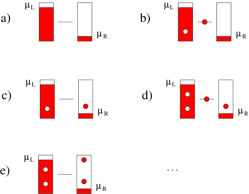
We identify the empty state |0ket0|0\rangle for the model with the condition of empty dot and leads filled up to their Fermi energies. Then we gradually move electrons from the emitter to the dot and finally to the collector and associate a new vector to each state of this “decaying chain”. We construct in this way an infinite many-body basis that defines the Hilbert space for the model101010Some of the possible states of the device are excluded from this Hilbert space: states with electrons excited above the Fermi level of the left lead and/or holes below the Fermi energy of the right lead. They are neglected because they would anyway be hardly populated due to the fast relaxation of the leads to their thermal states and the very low probability of electron tunneling for energies so far from the resonant level of the dot.. The first few elements of the basis read:

|0c1cl1|0cr1cl1|0c1cr1cl1cl2|0cr2cr1cl1cl2|0ket0superscriptsubscript𝑐1superscriptsubscript𝑐subscript𝑙1absentket0superscriptsubscript𝑐subscript𝑟1superscriptsubscript𝑐subscript𝑙1absentket0superscriptsubscript𝑐1superscriptsubscript𝑐subscript𝑟1superscriptsubscript𝑐subscript𝑙1absentsuperscriptsubscript𝑐subscript𝑙2absentket0superscriptsubscript𝑐subscript𝑟2superscriptsubscript𝑐subscript𝑟1superscriptsubscript𝑐subscript𝑙1absentsuperscriptsubscript𝑐subscript𝑙2absentket0|0\rangle\qquad c_{1}^{\dagger}c_{l_{1}}^{\phantom{\dagger}}|0\rangle\qquad c_{r_{1}}^{\dagger}c_{l_{1}}^{\phantom{\dagger}}|0\rangle\qquad c_{1}^{\dagger}c_{r_{1}}^{\dagger}c_{l_{1}}^{\phantom{\dagger}}c_{l_{2}}^{\phantom{\dagger}}|0\rangle\qquad c_{r_{2}}^{\dagger}c_{r_{1}}^{\dagger}c_{l_{1}}^{\phantom{\dagger}}c_{l_{2}}^{\phantom{\dagger}}|0\rangle\,\ldots (3.27)

where we choose by convention to move all the creation operators to the left and the annihilation operators to the right. We also assume with the two groups that εli<εli+1subscript𝜀subscript𝑙𝑖subscript𝜀subscript𝑙𝑖1\varepsilon_{l_{i}}<\varepsilon_{l_{i+1}} and εri<εri+1subscript𝜀subscript𝑟𝑖subscript𝜀subscript𝑟𝑖1\varepsilon_{r_{i}}<\varepsilon_{r_{i+1}} to avoid double counting.

Refer to caption
Figure 3.1: Schematic representation of the first elements of the many-body basis for the single dot model. Electrons are progressively taken from the emitter and moved to the QD and finally to the collector. The vectors represented are in the order a)=|0{\rm a)}=|0\rangle, b)=c1cl1|0{\rm b)}=c_{1}^{\dagger}c_{l_{1}}|0\rangle, c)=cr1cl1|0{\rm c)}=c_{r_{1}}^{\dagger}c_{l_{1}}|0\rangle, d)=c1cr1cl1cl2|0{\rm d)}=c_{1}^{\dagger}c_{r_{1}}^{\dagger}c_{l_{1}}c_{l_{2}}|0\rangle, e)=cr2cr1cl1cl2|0{\rm e)}=c_{r_{2}}^{\dagger}c_{r_{1}}^{\dagger}c_{l_{1}}c_{l_{2}}|0\rangle.

The state of the model is described by the many-particle vector |Ψ(t)ketΨ𝑡|\Psi(t)\rangle which we can expand over the basis:

|Ψ(t)=[b0(t)+l1b1l1(t)c1cl1+l1,r1bl1r1(t)cr1cl1+l1<l2,r1b1l1l2r1(t)c1cr1cl1cl2+l1<l2,r1<r2bl1l2r1r2(t)cr2cr1cl1cl2+]|0ketΨ𝑡delimited-[]subscript𝑏0𝑡subscriptsubscript𝑙1subscript𝑏1subscript𝑙1𝑡superscriptsubscript𝑐1superscriptsubscript𝑐subscript𝑙1absentsubscriptsubscript𝑙1subscript𝑟1subscript𝑏subscript𝑙1subscript𝑟1𝑡superscriptsubscript𝑐subscript𝑟1superscriptsubscript𝑐subscript𝑙1absentsubscriptsubscript𝑙1subscript𝑙2subscript𝑟1subscript𝑏1subscript𝑙1subscript𝑙2subscript𝑟1𝑡superscriptsubscript𝑐1superscriptsubscript𝑐subscript𝑟1superscriptsubscript𝑐subscript𝑙1absentsuperscriptsubscript𝑐subscript𝑙2absentsubscriptformulae-sequencesubscript𝑙1subscript𝑙2subscript𝑟1subscript𝑟2subscript𝑏subscript𝑙1subscript𝑙2subscript𝑟1subscript𝑟2𝑡superscriptsubscript𝑐subscript𝑟2superscriptsubscript𝑐subscript𝑟1superscriptsubscript𝑐subscript𝑙1absentsuperscriptsubscript𝑐subscript𝑙2absentket0\begin{split}|\Psi(t)\rangle=&\Big{[}b_{0}(t)+\sum_{l_{1}}b_{1l_{1}}(t)c_{1}^{\dagger}c_{l_{1}}^{\phantom{\dagger}}+\sum_{l_{1},r_{1}}b_{l_{1}r_{1}}(t)c_{r_{1}}^{\dagger}c_{l_{1}}^{\phantom{\dagger}}\\ &+\!\sum_{l_{1}<l_{2},r_{1}}b_{1l_{1}l_{2}r_{1}}(t)c_{1}^{\dagger}c_{r_{1}}^{\dagger}c_{l_{1}}^{\phantom{\dagger}}c_{l_{2}}^{\phantom{\dagger}}+\!\sum_{l_{1}<l_{2},r_{1}<r_{2}}b_{l_{1}l_{2}r_{1}r_{2}}(t)c_{r_{2}}^{\dagger}c_{r_{1}}^{\dagger}c_{l_{1}}^{\phantom{\dagger}}c_{l_{2}}^{\phantom{\dagger}}+\ldots\Big{]}|0\rangle\end{split} (3.28)

3.3.2 Recursive equation of motion for the coefficients

The vector |Ψ(t)ketΨ𝑡|\Psi(t)\rangle obeys the Schrödinger equation i|Ψ˙(t)=H|Ψ(t)𝑖Planck-constant-over-2-piket˙Ψ𝑡𝐻ketΨ𝑡i\hbar|\dot{\Psi}(t)\rangle=H|\Psi(t)\rangle and we impose the initial condition |Ψ(0)=|0ketΨ0ket0|\Psi(0)\rangle=|0\rangle. In terms of the coefficients of the expansion (3.28) we obtain an infinite set of differential equations with the initial condition b0(0)=1subscript𝑏001b_{0}(0)=1 and all the other coefficients equal to 00 at time t=0𝑡0t=0.

Due to the quadratic form of the Hamiltonian, the infinite set of differential equations for the coefficients b𝑏b’s presents a recursive structure: each coefficient is linked in its equation of motion only to the previous and the next in the “decaying chain”(3.28). Since we are interested in keeping track of the state of the dot we condense the full system of equations into two equations for the generic coefficients b{lj}j=1n{rj}j=1n(t)subscript𝑏superscriptsubscriptsubscript𝑙𝑗𝑗1𝑛superscriptsubscriptsubscript𝑟𝑗𝑗1𝑛𝑡b_{\{l_{j}\}_{j=1}^{n}\{r_{j}\}_{j=1}^{n}}(t) and b1{lj}j=1n+1{rj}j=1n(t)subscript𝑏1superscriptsubscriptsubscript𝑙𝑗𝑗1𝑛1superscriptsubscriptsubscript𝑟𝑗𝑗1𝑛𝑡b_{1\{l_{j}\}_{j=1}^{n+1}\{r_{j}\}_{j=1}^{n}}(t):

ib˙{lj}j=1n{rj}j=1n=[k=1n(εrkεlk)]b{lj}j=1n{rj}j=1n+ln+1Ωln+1b1{lj}j=1n+1{rj}j=1n+k=1n(1)knΩrkb1{lj}j=1n{rj}j=1n\{rk}ib˙1{lj}j=1n+1{rj}j=1n=[ε1+k=1n(εrkεlk)εln+1]b1{lj}j=1n+1{rj}j=1n+rn+1Ωrn+1b{lj}j=1n+1{rj}j=1n+1+k=1n+1(1)kn1Ωlkb{lj}j=1n+1\{lk}{rj}j=1n𝑖subscript˙𝑏superscriptsubscriptsubscript𝑙𝑗𝑗1𝑛superscriptsubscriptsubscript𝑟𝑗𝑗1𝑛delimited-[]superscriptsubscript𝑘1𝑛subscript𝜀subscript𝑟𝑘subscript𝜀subscript𝑙𝑘subscript𝑏superscriptsubscriptsubscript𝑙𝑗𝑗1𝑛superscriptsubscriptsubscript𝑟𝑗𝑗1𝑛subscriptsubscript𝑙𝑛1subscriptΩsubscript𝑙𝑛1subscript𝑏1superscriptsubscriptsubscript𝑙𝑗𝑗1𝑛1superscriptsubscriptsubscript𝑟𝑗𝑗1𝑛superscriptsubscript𝑘1𝑛superscript1𝑘𝑛subscriptΩsubscript𝑟𝑘subscript𝑏\1superscriptsubscriptsubscript𝑙𝑗𝑗1𝑛superscriptsubscriptsubscript𝑟𝑗𝑗1𝑛subscript𝑟𝑘𝑖subscript˙𝑏1superscriptsubscriptsubscript𝑙𝑗𝑗1𝑛1superscriptsubscriptsubscript𝑟𝑗𝑗1𝑛delimited-[]subscript𝜀1superscriptsubscript𝑘1𝑛subscript𝜀subscript𝑟𝑘subscript𝜀subscript𝑙𝑘subscript𝜀subscript𝑙𝑛1subscript𝑏1superscriptsubscriptsubscript𝑙𝑗𝑗1𝑛1superscriptsubscriptsubscript𝑟𝑗𝑗1𝑛subscriptsubscript𝑟𝑛1subscriptΩsubscript𝑟𝑛1subscript𝑏superscriptsubscriptsubscript𝑙𝑗𝑗1𝑛1superscriptsubscriptsubscript𝑟𝑗𝑗1𝑛1superscriptsubscript𝑘1𝑛1superscript1𝑘𝑛1subscriptΩsubscript𝑙𝑘subscript𝑏\superscriptsubscriptsubscript𝑙𝑗𝑗1𝑛1subscript𝑙𝑘superscriptsubscriptsubscript𝑟𝑗𝑗1𝑛\begin{split}i\dot{b}_{\{l_{j}\}_{j=1}^{n}\{r_{j}\}_{j=1}^{n}}=&\left[\sum_{k=1}^{n}(\varepsilon_{r_{k}}-\varepsilon_{l_{k}})\right]b_{\{l_{j}\}_{j=1}^{n}\{r_{j}\}_{j=1}^{n}}\\ &\!\!\!\!+\sum_{l_{n+1}}\Omega_{l_{n+1}}b_{1\{l_{j}\}_{j=1}^{n+1}\{r_{j}\}_{j=1}^{n}}+\sum_{k=1}^{n}(-1)^{k-n}\Omega_{r_{k}}b_{1\{l_{j}\}_{j=1}^{n}\{r_{j}\}_{j=1}^{n}\backslash\{r_{k}\}}\\ i\dot{b}_{1\{l_{j}\}_{j=1}^{n+1}\{r_{j}\}_{j=1}^{n}}=&\left[\varepsilon_{1}+\sum_{k=1}^{n}(\varepsilon_{r_{k}}-\varepsilon_{l_{k}})-\varepsilon_{l_{n+1}}\right]b_{1\{l_{j}\}_{j=1}^{n+1}\{r_{j}\}_{j=1}^{n}}\\ &\!\!\!\!+\sum_{r_{n+1}}\Omega_{r_{n+1}}b_{\{l_{j}\}_{j=1}^{n+1}\{r_{j}\}_{j=1}^{n+1}}+\sum_{k=1}^{n+1}(-1)^{k-n-1}\Omega_{l_{k}}b_{\{l_{j}\}_{j=1}^{n+1}\backslash\{l_{k}\}\{r_{j}\}_{j=1}^{n}}\\ \end{split} (3.29)

where =1Planck-constant-over-2-pi1\hbar=1 and the sums over labels (e.g. ln+1subscriptsubscript𝑙𝑛1\sum_{l_{n+1}}) are continuous sums over all the possible energy levels of the leads. We also used the shortened notations:

b{lj}j=1n{rj}j=1nbl1l2l3lnr1r2r3rn(t)b1{lj}j=1n+1\{lk}{rj}j=1nb1l1l2l3lk1lk+1ln+1r1r2r3rn(t)subscript𝑏superscriptsubscriptsubscript𝑙𝑗𝑗1𝑛superscriptsubscriptsubscript𝑟𝑗𝑗1𝑛subscript𝑏subscript𝑙1subscript𝑙2subscript𝑙3subscript𝑙𝑛subscript𝑟1subscript𝑟2subscript𝑟3subscript𝑟𝑛𝑡subscript𝑏\1superscriptsubscriptsubscript𝑙𝑗𝑗1𝑛1subscript𝑙𝑘superscriptsubscriptsubscript𝑟𝑗𝑗1𝑛subscript𝑏1subscript𝑙1subscript𝑙2subscript𝑙3subscript𝑙𝑘1subscript𝑙𝑘1subscript𝑙𝑛1subscript𝑟1subscript𝑟2subscript𝑟3subscript𝑟𝑛𝑡\begin{split}b_{\{l_{j}\}_{j=1}^{n}\{r_{j}\}_{j=1}^{n}}&\equiv b_{l_{1}l_{2}l_{3}\ldots l_{n}r_{1}r_{2}r_{3}\ldots r_{n}}(t)\\ b_{1\{l_{j}\}_{j=1}^{n+1}\backslash\{l_{k}\}\{r_{j}\}_{j=1}^{n}}&\equiv b_{1l_{1}l_{2}l_{3}\ldots l_{k-1}l_{k+1}\ldots l_{n+1}r_{1}r_{2}r_{3}\ldots r_{n}}(t)\end{split} (3.30)

In order to proceed in the derivation of the rate equations it is most convenient to make the Laplace transform of the system of differential equations (3.29). We obtain the system of algebraic equations:

[E+k=1n(εlkεrk)]b~{lj}j=1n{rj}j=1n(E)ln+1Ωln+1b~1{lj}j=1n+1{rj}j=1n(E)k=1n(1)knΩrkb~1{lj}j=1n{rj}j=1n\{rk}(E)=iδn0[Eε1+k=1n(εlkεrk)+εln+1]b~1{lj}j=1n+1{rj}j=1n(E)rn+1Ωrn+1b~{lj}j=1n+1{rj}j=1n+1(E)k=1n+1(1)kn1Ωlkb~{lj}j=1n+1\{lk}{rj}j=1n(E)=0delimited-[]𝐸superscriptsubscript𝑘1𝑛subscript𝜀subscript𝑙𝑘subscript𝜀subscript𝑟𝑘subscript~𝑏superscriptsubscriptsubscript𝑙𝑗𝑗1𝑛superscriptsubscriptsubscript𝑟𝑗𝑗1𝑛𝐸subscriptsubscript𝑙𝑛1subscriptΩsubscript𝑙𝑛1subscript~𝑏1superscriptsubscriptsubscript𝑙𝑗𝑗1𝑛1superscriptsubscriptsubscript𝑟𝑗𝑗1𝑛𝐸superscriptsubscript𝑘1𝑛superscript1𝑘𝑛subscriptΩsubscript𝑟𝑘subscript~𝑏\1superscriptsubscriptsubscript𝑙𝑗𝑗1𝑛superscriptsubscriptsubscript𝑟𝑗𝑗1𝑛subscript𝑟𝑘𝐸𝑖subscript𝛿𝑛0delimited-[]𝐸subscript𝜀1superscriptsubscript𝑘1𝑛subscript𝜀subscript𝑙𝑘subscript𝜀subscript𝑟𝑘subscript𝜀subscript𝑙𝑛1subscript~𝑏1superscriptsubscriptsubscript𝑙𝑗𝑗1𝑛1superscriptsubscriptsubscript𝑟𝑗𝑗1𝑛𝐸subscriptsubscript𝑟𝑛1subscriptΩsubscript𝑟𝑛1subscript~𝑏superscriptsubscriptsubscript𝑙𝑗𝑗1𝑛1superscriptsubscriptsubscript𝑟𝑗𝑗1𝑛1𝐸superscriptsubscript𝑘1𝑛1superscript1𝑘𝑛1subscriptΩsubscript𝑙𝑘subscript~𝑏\superscriptsubscriptsubscript𝑙𝑗𝑗1𝑛1subscript𝑙𝑘superscriptsubscriptsubscript𝑟𝑗𝑗1𝑛𝐸0\begin{split}&\left[E+\sum_{k=1}^{n}(\varepsilon_{l_{k}}-\varepsilon_{r_{k}})\right]\tilde{b}_{\{l_{j}\}_{j=1}^{n}\{r_{j}\}_{j=1}^{n}}(E)\\ &-\sum_{l_{n+1}}\Omega_{l_{n+1}}\tilde{b}_{1\{l_{j}\}_{j=1}^{n+1}\{r_{j}\}_{j=1}^{n}}(E)-\sum_{k=1}^{n}(-1)^{k-n}\Omega_{r_{k}}\tilde{b}_{1\{l_{j}\}_{j=1}^{n}\{r_{j}\}_{j=1}^{n}\backslash\{r_{k}\}}(E)=i\delta_{n0}\\ &\left[E-\varepsilon_{1}+\sum_{k=1}^{n}(\varepsilon_{l_{k}}-\varepsilon_{r_{k}})+\varepsilon_{l_{n+1}}\right]\tilde{b}_{1\{l_{j}\}_{j=1}^{n+1}\{r_{j}\}_{j=1}^{n}}(E)\\ &-\sum_{r_{n+1}}\Omega_{r_{n+1}}\tilde{b}_{\{l_{j}\}_{j=1}^{n+1}\{r_{j}\}_{j=1}^{n+1}}(E)-\sum_{k=1}^{n+1}(-1)^{k-n-1}\Omega_{l_{k}}\tilde{b}_{\{l_{j}\}_{j=1}^{n+1}\backslash\{l_{k}\}\{r_{j}\}_{j=1}^{n}}(E)=0\\ \end{split} (3.31)

where the Laplace transformed coefficients are indicated with a tilde and are functions of the variable E𝐸E (that we assume to have an imaginary part to ensure convergence of the Laplace integral). At this level the left-right asymmetry reveals itself in the number of “decay channels”. Each state of the chain (3.27) is coupled to an infinite number of right states and only a finite number of left states. Since the couplings are equivalent this results in a statistically definite direction of motion for the electrons.

3.3.3 Injection and ejection rates

The continuous sums in (3.31) can be simplified using the recursive structure of the equation of motion. We isolate in the second equation of (3.31) the coefficient b~1{lj}j=1n+1{rj}j=1n(E)subscript~𝑏1superscriptsubscriptsubscript𝑙𝑗𝑗1𝑛1superscriptsubscriptsubscript𝑟𝑗𝑗1𝑛𝐸\tilde{b}_{1\{l_{j}\}_{j=1}^{n+1}\{r_{j}\}_{j=1}^{n}}(E) and insert the result into the first equation of (3.31). The continuous sum results into two terms:

ln+1rn+1Ωln+1Ωrn+1Eε1+k=1n(εlkεrk)+εln+1b~{lj}j=1n+1{rj}j=1n+1subscriptsubscript𝑙𝑛1subscriptsubscript𝑟𝑛1subscriptΩsubscript𝑙𝑛1subscriptΩsubscript𝑟𝑛1𝐸subscript𝜀1superscriptsubscript𝑘1𝑛subscript𝜀subscript𝑙𝑘subscript𝜀subscript𝑟𝑘subscript𝜀subscript𝑙𝑛1subscript~𝑏superscriptsubscriptsubscript𝑙𝑗𝑗1𝑛1superscriptsubscriptsubscript𝑟𝑗𝑗1𝑛1\sum_{l_{n+1}}\sum_{r_{n+1}}\frac{\Omega_{l_{n+1}}\Omega_{r_{n+1}}}{E-\varepsilon_{1}+\sum_{k=1}^{n}(\varepsilon_{l_{k}}-\varepsilon_{r_{k}})+\varepsilon_{l_{n+1}}}\tilde{b}_{\{l_{j}\}_{j=1}^{n+1}\{r_{j}\}_{j=1}^{n+1}} (3.32)

and

ln+1k=1n+1(1)kn1Ωln+1ΩlkEε1+i=1n(εliεri)+εln+1b~{lj}j=1n+1\{lk}{rj}j=1nsubscriptsubscript𝑙𝑛1superscriptsubscript𝑘1𝑛1superscript1𝑘𝑛1subscriptΩsubscript𝑙𝑛1subscriptΩsubscript𝑙𝑘𝐸subscript𝜀1superscriptsubscript𝑖1𝑛subscript𝜀subscript𝑙𝑖subscript𝜀subscript𝑟𝑖subscript𝜀subscript𝑙𝑛1subscript~𝑏\superscriptsubscriptsubscript𝑙𝑗𝑗1𝑛1subscript𝑙𝑘superscriptsubscriptsubscript𝑟𝑗𝑗1𝑛\sum_{l_{n+1}}\sum_{k=1}^{n+1}(-1)^{k-n-1}\frac{\Omega_{l_{n+1}}\Omega_{l_{k}}}{E-\varepsilon_{1}+\sum_{i=1}^{n}(\varepsilon_{l_{i}}-\varepsilon_{r_{i}})+\varepsilon_{l_{n+1}}}\tilde{b}_{\{l_{j}\}_{j=1}^{n+1}\backslash\{l_{k}\}\{r_{j}\}_{j=1}^{n}} (3.33)

Since the energy levels in the leads are dense we can substitute

ln+1+𝑑εln+1DL(εln+1)subscriptsubscript𝑙𝑛1superscriptsubscriptdifferential-dsubscript𝜀subscript𝑙𝑛1subscript𝐷𝐿subscript𝜀subscript𝑙𝑛1\sum_{l_{n+1}}\to\int_{-\infty}^{+\infty}d\varepsilon_{l_{n+1}}D_{L}(\varepsilon_{l_{n+1}}) (3.34)

where D(εln+1)𝐷subscript𝜀subscript𝑙𝑛1D(\varepsilon_{l_{n+1}}) is the density of states in the left lead calculated at energy εln+1subscript𝜀subscript𝑙𝑛1\varepsilon_{l_{n+1}} and we have extended the integration limits to infinity in the wide band and high bias approximation. We can evaluate now the sum over ln+1subscript𝑙𝑛1l_{n+1} in (3.32) and (3.33) using residues method. Since all the poles are in the same half plane we can neglect all terms which are asymptotically o(|εln+1|1)𝑜superscriptsubscript𝜀subscript𝑙𝑛11o(|\varepsilon_{l_{n+1}}|^{-1}) for |εln+1|subscript𝜀subscript𝑙𝑛1|\varepsilon_{l_{n+1}}|\to\infty. It is clear from the algebraic system (3.31) that a coefficient b~~𝑏\tilde{b} that has among its indices εln+1subscript𝜀subscript𝑙𝑛1\varepsilon_{l_{n+1}} behaves asymptotically at least like |εln+1|1superscriptsubscript𝜀subscript𝑙𝑛11|\varepsilon_{l_{n+1}}|^{-1}. For this reason (3.32) vanishes and only one term is left from (3.33):

b~{lj}j=1n{rj}j=1n+𝑑εl+1DL(εln+1)Ωln+12Eε1+i=1n(εliεri)+εln+1subscript~𝑏superscriptsubscriptsubscript𝑙𝑗𝑗1𝑛superscriptsubscriptsubscript𝑟𝑗𝑗1𝑛superscriptsubscriptdifferential-dsubscript𝜀𝑙1subscript𝐷𝐿subscript𝜀subscript𝑙𝑛1superscriptsubscriptΩsubscript𝑙𝑛12𝐸subscript𝜀1superscriptsubscript𝑖1𝑛subscript𝜀subscript𝑙𝑖subscript𝜀subscript𝑟𝑖subscript𝜀subscript𝑙𝑛1\tilde{b}_{\{l_{j}\}_{j=1}^{n}\{r_{j}\}_{j=1}^{n}}\int_{-\infty}^{+\infty}d\varepsilon_{l+1}D_{L}(\varepsilon_{l_{n+1}})\frac{\Omega_{l_{n+1}}^{2}}{E-\varepsilon_{1}+\sum_{i=1}^{n}(\varepsilon_{l_{i}}-\varepsilon_{r_{i}})+\varepsilon_{l_{n+1}}} (3.35)

For the evaluation of the integral is enough that the tunneling amplitude Ωln+1subscriptΩsubscript𝑙𝑛1\Omega_{l_{n+1}} and the density of states DL(εln+1)subscript𝐷𝐿subscript𝜀subscript𝑙𝑛1D_{L}(\varepsilon_{l_{n+1}}) are analytical and non-zero where the denominator vanishes. We assume that they are constant to avoid n𝑛n-dependence in the tunneling rates and perform the integral in (3.35). The second equation (3.31) can be treated analogously and the system reads:

[E+k=1n(εlkεrk)+iΓL2]b~{lj}j=1n{rj}j=1n(E)k=1n(1)knΩrkb~1{lj}j=1n{rj}j=1n\{rk}(E)=iδn0[Eε1+k=1n(εlkεrk)+εln+1+iΓR2]b~1{lj}j=1n+1{rj}j=1n(E)k=1n+1(1)kn1Ωlkb~{lj}j=1n+1\{lk}{rj}j=1n(E)=0delimited-[]𝐸superscriptsubscript𝑘1𝑛subscript𝜀subscript𝑙𝑘subscript𝜀subscript𝑟𝑘𝑖subscriptΓ𝐿2subscript~𝑏superscriptsubscriptsubscript𝑙𝑗𝑗1𝑛superscriptsubscriptsubscript𝑟𝑗𝑗1𝑛𝐸superscriptsubscript𝑘1𝑛superscript1𝑘𝑛subscriptΩsubscript𝑟𝑘subscript~𝑏\1superscriptsubscriptsubscript𝑙𝑗𝑗1𝑛superscriptsubscriptsubscript𝑟𝑗𝑗1𝑛subscript𝑟𝑘𝐸𝑖subscript𝛿𝑛0delimited-[]𝐸subscript𝜀1superscriptsubscript𝑘1𝑛subscript𝜀subscript𝑙𝑘subscript𝜀subscript𝑟𝑘subscript𝜀subscript𝑙𝑛1𝑖subscriptΓ𝑅2subscript~𝑏1superscriptsubscriptsubscript𝑙𝑗𝑗1𝑛1superscriptsubscriptsubscript𝑟𝑗𝑗1𝑛𝐸superscriptsubscript𝑘1𝑛1superscript1𝑘𝑛1subscriptΩsubscript𝑙𝑘subscript~𝑏\superscriptsubscriptsubscript𝑙𝑗𝑗1𝑛1subscript𝑙𝑘superscriptsubscriptsubscript𝑟𝑗𝑗1𝑛𝐸0\begin{split}&\left[E+\sum_{k=1}^{n}(\varepsilon_{l_{k}}-\varepsilon_{r_{k}})+i\frac{\Gamma_{L}}{2}\right]\tilde{b}_{\{l_{j}\}_{j=1}^{n}\{r_{j}\}_{j=1}^{n}}(E)\\ &\phantom{aaaaa}-\sum_{k=1}^{n}(-1)^{k-n}\Omega_{r_{k}}\tilde{b}_{1\{l_{j}\}_{j=1}^{n}\{r_{j}\}_{j=1}^{n}\backslash\{r_{k}\}}(E)=i\delta_{n0}\\ &\left[E-\varepsilon_{1}+\sum_{k=1}^{n}(\varepsilon_{l_{k}}-\varepsilon_{r_{k}})+\varepsilon_{l_{n+1}}+i\frac{\Gamma_{R}}{2}\right]\tilde{b}_{1\{l_{j}\}_{j=1}^{n+1}\{r_{j}\}_{j=1}^{n}}(E)\\ &\phantom{aaaaa}-\sum_{k=1}^{n+1}(-1)^{k-n-1}\Omega_{l_{k}}\tilde{b}_{\{l_{j}\}_{j=1}^{n+1}\backslash\{l_{k}\}\{r_{j}\}_{j=1}^{n}}(E)=0\\ \end{split} (3.36)

where we have introduced the injection and ejection rates ΓLsubscriptΓ𝐿\Gamma_{L} and ΓRsubscriptΓ𝑅\Gamma_{R}

ΓL2πDLΩL2ΓR2πDRΩR2subscriptΓ𝐿2𝜋subscript𝐷𝐿superscriptsubscriptΩ𝐿2subscriptΓ𝑅2𝜋subscript𝐷𝑅superscriptsubscriptΩ𝑅2\begin{split}\Gamma_{L}&\equiv 2\pi D_{L}\Omega_{L}^{2}\\ \Gamma_{R}&\equiv 2\pi D_{R}\Omega_{R}^{2}\end{split} (3.37)

whith the energy independent tunneling amplitudes (ΩLsubscriptΩ𝐿\Omega_{L} and ΩRsubscriptΩ𝑅\Omega_{R}) and density of states (DLsubscript𝐷𝐿D_{L} and DRsubscript𝐷𝑅D_{R})111111We assume real tunneling amplitudes as it is also implied by the form of the Hamiltonian (3.26). The most general case of complex amplitude would result anyway in the tunneling rates ΓL,R2πDL,R|ΩL,R|2subscriptΓ𝐿𝑅2𝜋subscript𝐷𝐿𝑅superscriptsubscriptΩ𝐿𝑅2\Gamma_{L,R}\equiv 2\pi D_{L,R}|\Omega_{L,R}|^{2}..

3.3.4 The reduced density matrix

The reduced density operator is defined as the trace over the bath variables of the total density operator:

σ(t)=TrB{|Ψ(t)Ψ(t)|}𝜎𝑡subscriptTr𝐵ketΨ𝑡braΨ𝑡\sigma(t)={\rm Tr}_{B}\{|\Psi(t)\rangle\!\langle\Psi(t)|\} (3.38)

The matrix elements of the reduced density operators are explicitly

σij(t)={B}iS,B|Ψ(t)Ψ(t)|B,jSsubscript𝜎𝑖𝑗𝑡subscript𝐵inner-productsubscript𝑖𝑆𝐵Ψ𝑡inner-productΨ𝑡𝐵subscript𝑗𝑆\sigma_{ij}(t)=\sum_{\{B\}}\langle i_{S},B|\Psi(t)\rangle\!\langle\Psi(t)|B,j_{S}\rangle (3.39)

where |iS,B,i=0,1formulae-sequenceketsubscript𝑖𝑆𝐵𝑖01|i_{S},B\rangle,i=0,1 is the vector that corresponds to the empty or charged dot (the system) and a particular configuration B𝐵B of the leads (the baths). We assume that the bath state B𝐵B does not contain coherent superpositions of states with different number of particles. This implies the vanishing of coherencies in the reduced density matrix. It is useful to organize the sum over the bath configurations according to the number of extra electrons (holes) collected into the right (left) lead.

σii(t)=n=0{Bn}iS,Bn|Ψ(t)Ψ(t)|Bn,iS=n=0σii(n)(t)subscript𝜎𝑖𝑖𝑡superscriptsubscript𝑛0subscriptsubscript𝐵𝑛inner-productsubscript𝑖𝑆subscript𝐵𝑛Ψ𝑡inner-productΨ𝑡subscript𝐵𝑛subscript𝑖𝑆superscriptsubscript𝑛0superscriptsubscript𝜎𝑖𝑖𝑛𝑡\sigma_{ii}(t)=\sum_{n=0}^{\infty}\sum_{\{B_{n}\}}\langle i_{S},B_{n}|\Psi(t)\rangle\!\langle\Psi(t)|B_{n},i_{S}\rangle=\sum_{n=0}^{\infty}\sigma_{ii}^{(n)}(t) (3.40)

where Bnsubscript𝐵𝑛B_{n} is a configuration of the baths with n𝑛n extra electrons in the collector and we have introduced the n-resolved density matrix σ(n)superscript𝜎𝑛\sigma^{(n)}. Using the expansion of the vector |Ψ(t)ketΨ𝑡|\Psi(t)\rangle in the many-body basis (3.27) we can express the n𝑛n-resolved density matrix in terms of the coefficients b𝑏b. For the two non-vanishing elements:

σ00(n)={Bn}|0S,Bn|Ψ(t)|2={lk}{rk}|b{lk}k=1n{rk}k=1n(t)|2σ11(n)={Bn}|1S,Bn|Ψ(t)|2={lk}{rk}|b1{lk}k=1n+1{rk}k=1n(t)|2superscriptsubscript𝜎00𝑛subscriptsubscript𝐵𝑛superscriptinner-productsubscript0𝑆subscript𝐵𝑛Ψ𝑡2subscriptsubscript𝑙𝑘subscript𝑟𝑘superscriptsubscript𝑏superscriptsubscriptsubscript𝑙𝑘𝑘1𝑛superscriptsubscriptsubscript𝑟𝑘𝑘1𝑛𝑡2superscriptsubscript𝜎11𝑛subscriptsubscript𝐵𝑛superscriptinner-productsubscript1𝑆subscript𝐵𝑛Ψ𝑡2subscriptsubscript𝑙𝑘subscript𝑟𝑘superscriptsubscript𝑏1superscriptsubscriptsubscript𝑙𝑘𝑘1𝑛1superscriptsubscriptsubscript𝑟𝑘𝑘1𝑛𝑡2\begin{split}\sigma_{00}^{(n)}&=\sum_{\{B_{n}\}}|\langle 0_{S},B_{n}|\Psi(t)\rangle|^{2}=\sum_{\{l_{k}\}\{r_{k}\}}|b_{\{l_{k}\}_{k=1}^{n}\{r_{k}\}_{k=1}^{n}}(t)|^{2}\\ \sigma_{11}^{(n)}&=\sum_{\{B_{n}\}}|\langle 1_{S},B_{n}|\Psi(t)\rangle|^{2}=\sum_{\{l_{k}\}\{r_{k}\}}|b_{1\{l_{k}\}_{k=1}^{n+1}\{r_{k}\}_{k=1}^{n}}(t)|^{2}\end{split} (3.41)

where the sums are calculated over all the possible configurations of indistinguishable particles (e.g. {lk}l1<l2<l3<<lnsubscriptsubscript𝑙𝑘subscriptsubscript𝑙1subscript𝑙2subscript𝑙3subscript𝑙𝑛\sum_{\{l_{k}\}}\equiv\sum_{l_{1}<l_{2}<l_{3}<\ldots<l_{n}}). The time-dependent matrix elements of the reduced density matrix are connected to the coefficients b~(E)~𝑏𝐸\tilde{b}(E) by the inverse of the Laplace transform:

σ00(n)(t)={lk}{rk}dEdE4π2b~{lk}k=1n{rk}k=1n(E)b~{lk}k=1n{rk}k=1n(E)ei(EE)tσ11(n)(t)={lk}{rk}dEdE4π2b~1{lk}k=1n+1{rk}k=1n(E)b~1{lk}k=1n+1{rk}k=1n(E)ei(EE)tsubscriptsuperscript𝜎𝑛00𝑡subscriptsubscript𝑙𝑘subscript𝑟𝑘𝑑𝐸𝑑superscript𝐸4superscript𝜋2subscript~𝑏superscriptsubscriptsubscript𝑙𝑘𝑘1𝑛superscriptsubscriptsubscript𝑟𝑘𝑘1𝑛𝐸subscriptsuperscript~𝑏superscriptsubscriptsubscript𝑙𝑘𝑘1𝑛superscriptsubscriptsubscript𝑟𝑘𝑘1𝑛superscript𝐸superscript𝑒𝑖𝐸superscript𝐸𝑡subscriptsuperscript𝜎𝑛11𝑡subscriptsubscript𝑙𝑘subscript𝑟𝑘𝑑𝐸𝑑superscript𝐸4superscript𝜋2subscript~𝑏1superscriptsubscriptsubscript𝑙𝑘𝑘1𝑛1superscriptsubscriptsubscript𝑟𝑘𝑘1𝑛𝐸subscriptsuperscript~𝑏1superscriptsubscriptsubscript𝑙𝑘𝑘1𝑛1superscriptsubscriptsubscript𝑟𝑘𝑘1𝑛superscript𝐸superscript𝑒𝑖𝐸superscript𝐸𝑡\begin{split}\sigma^{(n)}_{00}(t)&=\sum_{\{l_{k}\}\{r_{k}\}}\int\frac{dEdE^{\prime}}{4\pi^{2}}\tilde{b}_{\{l_{k}\}_{k=1}^{n}\{r_{k}\}_{k=1}^{n}}(E)\tilde{b}^{*}_{\{l_{k}\}_{k=1}^{n}\{r_{k}\}_{k=1}^{n}}(E^{\prime})e^{i(E-E^{\prime})t}\\ \sigma^{(n)}_{11}(t)&=\sum_{\{l_{k}\}\{r_{k}\}}\int\frac{dEdE^{\prime}}{4\pi^{2}}\tilde{b}_{1\{l_{k}\}_{k=1}^{n+1}\{r_{k}\}_{k=1}^{n}}(E)\tilde{b}^{*}_{1\{l_{k}\}_{k=1}^{n+1}\{r_{k}\}_{k=1}^{n}}(E^{\prime})e^{i(E-E^{\prime})t}\\ \end{split} (3.42)

Apart from being a natural step in the derivation of the GME in the Gurvitz approach, the n𝑛n-resolved density matrix contains the additional information on the number of electrons collected in the resevoir at time t𝑡t. This information is very useful to the calculation of the current noise in the SDQS where the quantum regression theorem can not be applied due to the form of the current operator that involves both system and bath operators.

3.3.5 Generalized Master Equation

The equation of motion for the reduced density matrix is obtained combining (3.42) and (3.36). First we derive an equation of motion for the n𝑛n-resolved reduced density matrix σ(n)superscript𝜎𝑛\sigma^{(n)}. The case of the empty dot population with n=0𝑛0n=0 is special due to the particular choice of the initial condition and we treat it separately. The starting point is the first of the equations (3.36) specialized for n=0𝑛0n=0, namely:

(E+iΓL2)b~0(E)=i𝐸𝑖subscriptΓ𝐿2subscript~𝑏0𝐸𝑖\left(E+i\frac{\Gamma_{L}}{2}\right)\tilde{b}_{0}(E)=i (3.43)

We taking the inverse Laplace transform and obtain

b˙0(t)=ΓL2b0(t)subscript˙𝑏0𝑡subscriptΓ𝐿2subscript𝑏0𝑡\dot{b}_{0}(t)=-\frac{\Gamma_{L}}{2}b_{0}(t) (3.44)

The definition of σ00(0)superscriptsubscript𝜎000\sigma_{00}^{(0)} and the Leibnitz theorem for derivatives lead to the conclusion:

σ˙00(0)=b˙0b0+b0b˙0=ΓLb0b0=ΓLσ00(0)superscriptsubscript˙𝜎000subscript˙𝑏0superscriptsubscript𝑏0subscript𝑏0superscriptsubscript˙𝑏0subscriptΓ𝐿subscript𝑏0superscriptsubscript𝑏0subscriptΓ𝐿superscriptsubscript𝜎000\dot{\sigma}_{00}^{(0)}=\dot{b}_{0}b_{0}^{*}+b_{0}\dot{b}_{0}^{*}=-\Gamma_{L}b_{0}b_{0}^{*}=-\Gamma_{L}\sigma_{00}^{(0)} (3.45)

This argument is applied also in the case with n0𝑛0n\neq 0 but the structure of the equation is more complex and in general a final continuous sum must be evaluated. We take the first equation in (3.36) and multiply it by b~{lj}j=1n{rj}j=1n(E)subscriptsuperscript~𝑏superscriptsubscriptsubscript𝑙𝑗𝑗1𝑛superscriptsubscriptsubscript𝑟𝑗𝑗1𝑛superscript𝐸\tilde{b}^{*}_{\{l_{j}\}_{j=1}^{n}\{r_{j}\}_{j=1}^{n}}(E^{\prime})ei(EE)tsuperscript𝑒𝑖𝐸superscript𝐸𝑡e^{-i(E-E^{\prime})t}. Then we subtract side by side the complex conjugate of the first equation of (3.36) evaluated in Esuperscript𝐸E^{\prime} and multiplied by b~{lj}j=1n{rj}j=1n(E)subscript~𝑏superscriptsubscriptsubscript𝑙𝑗𝑗1𝑛superscriptsubscriptsubscript𝑟𝑗𝑗1𝑛𝐸\tilde{b}_{\{l_{j}\}_{j=1}^{n}\{r_{j}\}_{j=1}^{n}}(E)ei(EE)tsuperscript𝑒𝑖𝐸superscript𝐸𝑡e^{-i(E-E^{\prime})t}. Finally we integrate in dE𝑑𝐸dE and dE𝑑superscript𝐸dE^{\prime} and sum over the bath configurations with n𝑛n electrons in the collector. We repeat the procedure also for the second equation in (3.36) and obtain:

{lj}{rj}dEdE4π2[(EE+iΓL)b~{lj}j=1n{rj}j=1n(E)b~{lj}j=1n{rj}j=1n(E)ei(EE)t2(k=1n(1)knΩrkb~1{lj}j=1n{rj}j=1n\{rk}(E)b~{lj}j=1n{rj}j=1n(E)ei(EE)t)]=0subscriptsubscript𝑙𝑗subscript𝑟𝑗𝑑𝐸𝑑superscript𝐸4superscript𝜋2delimited-[]𝐸superscript𝐸𝑖subscriptΓ𝐿subscript~𝑏superscriptsubscriptsubscript𝑙𝑗𝑗1𝑛superscriptsubscriptsubscript𝑟𝑗𝑗1𝑛𝐸subscriptsuperscript~𝑏superscriptsubscriptsubscript𝑙𝑗𝑗1𝑛superscriptsubscriptsubscript𝑟𝑗𝑗1𝑛superscript𝐸superscript𝑒𝑖𝐸superscript𝐸𝑡2superscriptsubscript𝑘1𝑛superscript1𝑘𝑛subscriptΩsubscript𝑟𝑘subscript~𝑏\1superscriptsubscriptsubscript𝑙𝑗𝑗1𝑛superscriptsubscriptsubscript𝑟𝑗𝑗1𝑛subscript𝑟𝑘𝐸subscriptsuperscript~𝑏superscriptsubscriptsubscript𝑙𝑗𝑗1𝑛superscriptsubscriptsubscript𝑟𝑗𝑗1𝑛superscript𝐸superscript𝑒𝑖𝐸superscript𝐸𝑡0\begin{split}&\sum_{\{l_{j}\}\{r_{j}\}}\!\int\frac{dEdE^{\prime}}{4\pi^{2}}\Big{[}(E-E^{\prime}+i\Gamma_{L})\tilde{b}_{\{l_{j}\}_{j=1}^{n}\{r_{j}\}_{j=1}^{n}}(E)\tilde{b}^{*}_{\{l_{j}\}_{j=1}^{n}\{r_{j}\}_{j=1}^{n}}\!(E^{\prime})e^{-i(E-E^{\prime})t}\\ &-2\Im\Big{(}\sum_{k=1}^{n}(-1)^{k-n}\Omega_{r_{k}}\tilde{b}_{1\{l_{j}\}_{j=1}^{n}\{r_{j}\}_{j=1}^{n}\backslash\{r_{k}\}}(E)\tilde{b}^{*}_{\{l_{j}\}_{j=1}^{n}\{r_{j}\}_{j=1}^{n}}(E^{\prime})e^{-i(E-E^{\prime})t}\Big{)}\Big{]}=0\end{split} (3.46)

for the first equation and similarly

{lj}{rj}dEdE4π2[(EE+iΓR)b~1{lj}j=1n+1{rj}j=1n(E)b~1{lj}j=1n+1{rj}j=1n(E)ei(EE)t2(k=1n+1(1)kn1Ωlkb~{lj}j=1n+1\{lk}{rj}j=1n(E)b~1{lj}j=1n+1{rj}j=1n(E)ei(EE)t)]=0subscriptsubscript𝑙𝑗subscript𝑟𝑗𝑑𝐸𝑑superscript𝐸4superscript𝜋2delimited-[]𝐸superscript𝐸𝑖subscriptΓ𝑅subscript~𝑏1superscriptsubscriptsubscript𝑙𝑗𝑗1𝑛1superscriptsubscriptsubscript𝑟𝑗𝑗1𝑛𝐸subscriptsuperscript~𝑏1superscriptsubscriptsubscript𝑙𝑗𝑗1𝑛1superscriptsubscriptsubscript𝑟𝑗𝑗1𝑛superscript𝐸superscript𝑒𝑖𝐸superscript𝐸𝑡2superscriptsubscript𝑘1𝑛1superscript1𝑘𝑛1subscriptΩsubscript𝑙𝑘subscript~𝑏\superscriptsubscriptsubscript𝑙𝑗𝑗1𝑛1subscript𝑙𝑘superscriptsubscriptsubscript𝑟𝑗𝑗1𝑛𝐸subscriptsuperscript~𝑏1superscriptsubscriptsubscript𝑙𝑗𝑗1𝑛1superscriptsubscriptsubscript𝑟𝑗𝑗1𝑛superscript𝐸superscript𝑒𝑖𝐸superscript𝐸𝑡0\begin{split}&\sum_{\{l_{j}\}\{r_{j}\}}\!\int\frac{dEdE^{\prime}}{4\pi^{2}}\Big{[}(E-E^{\prime}+i\Gamma_{R})\tilde{b}_{1\{l_{j}\}_{j=1}^{n+1}\{r_{j}\}_{j=1}^{n}}(E)\tilde{b}^{*}_{1\{l_{j}\}_{j=1}^{n+1}\{r_{j}\}_{j=1}^{n}}\!(E^{\prime})e^{-i(E-E^{\prime})t}\\ &-2\Im\Big{(}\sum_{k=1}^{n+1}(-1)^{k-n-1}\Omega_{l_{k}}\tilde{b}_{\{l_{j}\}_{j=1}^{n+1}\backslash\{l_{k}\}\{r_{j}\}_{j=1}^{n}}(E)\tilde{b}^{*}_{1\{l_{j}\}_{j=1}^{n+1}\{r_{j}\}_{j=1}^{n}}(E^{\prime})e^{-i(E-E^{\prime})t}\Big{)}\Big{]}=0\\ \end{split} (3.47)

for the second. \Im indicates the imaginary part. In the definition of the n𝑛n-resolved reduced density matrix the two coefficients b𝑏b correspond to the same bath configuration. The finite sums in equations (3.46) and (3.47) still have coefficients with different bath configuration. Using properties of the Laplace transform, the definition of σ(n)superscript𝜎𝑛\sigma^{(n)} and the relations

b~{lj}j=1n{rj}j=1n(E)=k=1n(1)knΩrkb~1{lj}j=1n{rj}j=1n\{rk}(E)E+k=1n(εlkεrk)iΓL2b~1{lj}j=1n+1{rj}j=1n(E)=k=1n+1(1)kn1Ωlkb~{lj}j=1n+1\{lk}{rj}j=1n(E)Eε1+k=1n(εlkεrk)+εln+1iΓR2subscriptsuperscript~𝑏superscriptsubscriptsubscript𝑙𝑗𝑗1𝑛superscriptsubscriptsubscript𝑟𝑗𝑗1𝑛superscript𝐸superscriptsubscript𝑘1𝑛superscript1𝑘𝑛subscriptΩsubscript𝑟𝑘subscriptsuperscript~𝑏\1superscriptsubscriptsubscript𝑙𝑗𝑗1𝑛superscriptsubscriptsubscript𝑟𝑗𝑗1𝑛subscript𝑟𝑘superscript𝐸superscript𝐸superscriptsubscript𝑘1𝑛subscript𝜀subscript𝑙𝑘subscript𝜀subscript𝑟𝑘𝑖subscriptΓ𝐿2subscriptsuperscript~𝑏1superscriptsubscriptsubscript𝑙𝑗𝑗1𝑛1superscriptsubscriptsubscript𝑟𝑗𝑗1𝑛superscript𝐸superscriptsubscript𝑘1𝑛1superscript1𝑘𝑛1subscriptΩsubscript𝑙𝑘subscriptsuperscript~𝑏\superscriptsubscriptsubscript𝑙𝑗𝑗1𝑛1subscript𝑙𝑘superscriptsubscriptsubscript𝑟𝑗𝑗1𝑛superscript𝐸superscript𝐸subscript𝜀1superscriptsubscript𝑘1𝑛subscript𝜀subscript𝑙𝑘subscript𝜀subscript𝑟𝑘subscript𝜀subscript𝑙𝑛1𝑖subscriptΓ𝑅2\begin{split}\tilde{b}^{*}_{\{l_{j}\}_{j=1}^{n}\{r_{j}\}_{j=1}^{n}}(E^{\prime})&=\frac{\sum_{k=1}^{n}(-1)^{k-n}\Omega_{r_{k}}\tilde{b}^{*}_{1\{l_{j}\}_{j=1}^{n}\{r_{j}\}_{j=1}^{n}\backslash\{r_{k}\}}(E^{\prime})}{E^{\prime}+\sum_{k=1}^{n}(\varepsilon_{l_{k}}-\varepsilon_{r_{k}})-i\frac{\Gamma_{L}}{2}}\\ \tilde{b}^{*}_{1\{l_{j}\}_{j=1}^{n+1}\{r_{j}\}_{j=1}^{n}}(E^{\prime})&=\frac{\sum_{k=1}^{n+1}(-1)^{k-n-1}\Omega_{l_{k}}\tilde{b}^{*}_{\{l_{j}\}_{j=1}^{n+1}\backslash\{l_{k}\}\{r_{j}\}_{j=1}^{n}}(E^{\prime})}{E^{\prime}-\varepsilon_{1}+\sum_{k=1}^{n}(\varepsilon_{l_{k}}-\varepsilon_{r_{k}})+\varepsilon_{l_{n+1}}-i\frac{\Gamma_{R}}{2}}\end{split} (3.48)

obtained from (3.36), we transform (3.46) and (3.47) into:

i(σ˙00(n)+ΓLσ00(n))={lj}{rj}dEdE4π2[2(k,k=1n(1)k+kΩrkΩrkE+k=1n(εlkεrk)iΓL2b~1{lj}j=1n{rj}j=1n\{rk}(E)b~1{lj}j=1n{rj}j=1n\{rk}(E)ei(EE)t)]𝑖superscriptsubscript˙𝜎00𝑛subscriptΓ𝐿superscriptsubscript𝜎00𝑛subscriptsubscript𝑙𝑗subscript𝑟𝑗𝑑𝐸𝑑superscript𝐸4superscript𝜋2delimited-[]2superscriptsubscript𝑘superscript𝑘1𝑛superscript1𝑘superscript𝑘subscriptΩsubscript𝑟𝑘subscriptΩsubscript𝑟superscript𝑘superscript𝐸superscriptsubscript𝑘1𝑛subscript𝜀subscript𝑙𝑘subscript𝜀subscript𝑟𝑘𝑖subscriptΓ𝐿2subscript~𝑏\1superscriptsubscriptsubscript𝑙𝑗𝑗1𝑛superscriptsubscriptsubscript𝑟𝑗𝑗1𝑛subscript𝑟𝑘𝐸subscriptsuperscript~𝑏\1superscriptsubscriptsubscript𝑙𝑗𝑗1𝑛superscriptsubscriptsubscript𝑟𝑗𝑗1𝑛subscript𝑟superscript𝑘superscript𝐸superscript𝑒𝑖𝐸superscript𝐸𝑡\begin{split}i(\dot{\sigma}_{00}^{(n)}+\Gamma_{L}\sigma_{00}^{(n)})=\phantom{\Big{[}2\Im\Big{(}\sum_{k,k^{\prime}=1}^{n}\frac{(-1)^{k+k^{\prime}}\Omega_{r_{k}}\Omega_{r_{k^{\prime}}}}{E^{\prime}+\sum_{k=1}^{n}(\varepsilon_{l_{k}}-\varepsilon_{r_{k}})-i\frac{\Gamma_{L}}{2}}}&\\ \sum_{\{l_{j}\}\{r_{j}\}}\int\frac{dEdE^{\prime}}{4\pi^{2}}\Big{[}2\Im\Big{(}\sum_{k,k^{\prime}=1}^{n}\frac{(-1)^{k+k^{\prime}}\Omega_{r_{k}}\Omega_{r_{k^{\prime}}}}{E^{\prime}+\sum_{k=1}^{n}(\varepsilon_{l_{k}}-\varepsilon_{r_{k}})-i\frac{\Gamma_{L}}{2}}&\\ \tilde{b}_{1\{l_{j}\}_{j=1}^{n}\{r_{j}\}_{j=1}^{n}\backslash\{r_{k}\}}(E)\tilde{b}^{*}_{1\{l_{j}\}_{j=1}^{n}\{r_{j}\}_{j=1}^{n}\backslash\{r_{k^{\prime}}\}}(E^{\prime})e^{-i(E-E^{\prime})t}\Big{)}\Big{]}&\end{split} (3.49)

and

i(σ˙11(n)+ΓRσ11(n))={lj}{rj}dEdE4π2[2(k,k=1n+1(1)k+kΩlkΩlkEε1+k=1n(εlkεrk+εln+1)iΓL2b~{lj}j=1n+1\{lk}{rj}j=1n(E)b~{lj}j=1n+1\{lk}{rj}j=1n(E)ei(EE)t)]𝑖superscriptsubscript˙𝜎11𝑛subscriptΓ𝑅superscriptsubscript𝜎11𝑛subscriptsubscript𝑙𝑗subscript𝑟𝑗𝑑𝐸𝑑superscript𝐸4superscript𝜋2delimited-[]2superscriptsubscript𝑘superscript𝑘1𝑛1superscript1𝑘superscript𝑘subscriptΩsubscript𝑙𝑘subscriptΩsubscript𝑙superscript𝑘superscript𝐸subscript𝜀1superscriptsubscript𝑘1𝑛subscript𝜀subscript𝑙𝑘subscript𝜀subscript𝑟𝑘subscript𝜀subscript𝑙𝑛1𝑖subscriptΓ𝐿2subscript~𝑏\superscriptsubscriptsubscript𝑙𝑗𝑗1𝑛1subscript𝑙𝑘superscriptsubscriptsubscript𝑟𝑗𝑗1𝑛𝐸subscriptsuperscript~𝑏\superscriptsubscriptsubscript𝑙𝑗𝑗1𝑛1subscript𝑙superscript𝑘superscriptsubscriptsubscript𝑟𝑗𝑗1𝑛superscript𝐸superscript𝑒𝑖𝐸superscript𝐸𝑡\begin{split}i(\dot{\sigma}_{11}^{(n)}+\Gamma_{R}\sigma_{11}^{(n)})=\phantom{\Big{[}2\Im\Big{(}\sum_{k,k^{\prime}=1}^{n+1}\frac{(-1)^{k+k^{\prime}}\Omega_{l_{k}}\Omega_{l_{k^{\prime}}}}{E^{\prime}-\varepsilon_{1}+\sum_{k=1}^{n}(\varepsilon_{l_{k}}-\varepsilon_{r_{k}}+\varepsilon_{l_{n+1}})-i\frac{\Gamma_{L}}{2}}}&\\ \sum_{\{l_{j}\}\{r_{j}\}}\int\frac{dEdE^{\prime}}{4\pi^{2}}\Big{[}2\Im\Big{(}\sum_{k,k^{\prime}=1}^{n+1}\frac{(-1)^{k+k^{\prime}}\Omega_{l_{k}}\Omega_{l_{k^{\prime}}}}{E^{\prime}-\varepsilon_{1}+\sum_{k=1}^{n}(\varepsilon_{l_{k}}-\varepsilon_{r_{k}}+\varepsilon_{l_{n+1}})-i\frac{\Gamma_{L}}{2}}&\\ \tilde{b}_{\{l_{j}\}_{j=1}^{n+1}\backslash\{l_{k}\}\{r_{j}\}_{j=1}^{n}}(E)\tilde{b}^{*}_{\{l_{j}\}_{j=1}^{n+1}\backslash\{l_{k^{\prime}}\}\{r_{j}\}_{j=1}^{n}}(E^{\prime})e^{-i(E-E^{\prime})t}\Big{)}\Big{]}&\end{split} (3.50)

It is crucial at this point that k=k𝑘superscript𝑘k=k^{\prime}. If kk𝑘superscript𝑘k\neq k^{\prime} we can eliminate the variables rksubscript𝑟𝑘r_{k} (lksubscript𝑙𝑘l_{k}) from b~~𝑏\tilde{b} and rksubscript𝑟superscript𝑘r_{k^{\prime}} (lksubscript𝑙superscript𝑘l_{k^{\prime}}) from b~superscript~𝑏\tilde{b}^{*}, perform the integral over one of the now common “missing” variables121212Missing in the sense that they have been eliminated from the coefficients subcripts. and obtain zero. We are left with the case k=k𝑘superscript𝑘k=k^{\prime}. We transform the sum over the “missing” variable rksubscript𝑟𝑘r_{k} (lksubscript𝑙𝑘l_{k}) into an integral in the corresponding energy. The discrete sum in the index k𝑘k takes care of the integration limits and sets them to infinity. The integral can be performed using residues methods to get:

i[σ˙00(n)(t)+ΓLσ00(n)(t)]=iΓR{lj}{rj}|b1{lj}j=1n{rj}j=1n1(t)|2i[σ˙11(n)(t)+ΓRσ11(n)(t)]=iΓL{lj}{rj}|b{lj}j=1n{rj}j=1n(t)|2𝑖delimited-[]superscriptsubscript˙𝜎00𝑛𝑡subscriptΓ𝐿superscriptsubscript𝜎00𝑛𝑡𝑖subscriptΓ𝑅subscriptsubscript𝑙𝑗subscript𝑟𝑗superscriptsubscript𝑏1superscriptsubscriptsubscript𝑙𝑗𝑗1𝑛superscriptsubscriptsubscript𝑟𝑗𝑗1𝑛1𝑡2𝑖delimited-[]superscriptsubscript˙𝜎11𝑛𝑡subscriptΓ𝑅superscriptsubscript𝜎11𝑛𝑡𝑖subscriptΓ𝐿subscriptsubscript𝑙𝑗subscript𝑟𝑗superscriptsubscript𝑏superscriptsubscriptsubscript𝑙𝑗𝑗1𝑛superscriptsubscriptsubscript𝑟𝑗𝑗1𝑛𝑡2\begin{split}i[\dot{\sigma}_{00}^{(n)}(t)+\Gamma_{L}\sigma_{00}^{(n)}(t)]&=i\Gamma_{R}\sum_{\{l_{j}\}\{r_{j}\}}|b_{1\{l_{j}\}_{j=1}^{n}\{r_{j}\}_{j=1}^{n-1}}(t)|^{2}\\ i[\dot{\sigma}_{11}^{(n)}(t)+\Gamma_{R}\sigma_{11}^{(n)}(t)]&=i\Gamma_{L}\sum_{\{l_{j}\}\{r_{j}\}}|b_{\{l_{j}\}_{j=1}^{n}\{r_{j}\}_{j=1}^{n}}(t)|^{2}\\ \end{split} (3.51)

Finally we use the representation of the n𝑛n-resolved reduced density matrix (3.41) and obtain the master equation:

σ˙00(n)=ΓLσ00(n)+ΓRσ11(n1)σ˙11(n)=ΓRσ11(n)+ΓLσ00(n)superscriptsubscript˙𝜎00𝑛subscriptΓ𝐿superscriptsubscript𝜎00𝑛subscriptΓ𝑅superscriptsubscript𝜎11𝑛1superscriptsubscript˙𝜎11𝑛subscriptΓ𝑅superscriptsubscript𝜎11𝑛subscriptΓ𝐿superscriptsubscript𝜎00𝑛\begin{split}\dot{\sigma}_{00}^{(n)}&=-\Gamma_{L}\sigma_{00}^{(n)}+\Gamma_{R}\sigma_{11}^{(n-1)}\\ \dot{\sigma}_{11}^{(n)}&=-\Gamma_{R}\sigma_{11}^{(n)}+\Gamma_{L}\sigma_{00}^{(n)}\end{split} (3.52)

where we assume that σ11(1)0superscriptsubscript𝜎1110\sigma_{11}^{(-1)}\equiv 0 to include into the same compact form also the equation (3.45) for n=0𝑛0n=0. From this set of equations it is possible to determine the current in the left and right leads. The current in the right lead is the time derivative of the total number of electrons collected in the right lead at time t𝑡t:

IR(t)=N˙R(t)=n=0n[σ˙00(n)(t)+σ˙11(n)(t)]subscript𝐼𝑅𝑡subscript˙𝑁𝑅𝑡superscriptsubscript𝑛0𝑛delimited-[]superscriptsubscript˙𝜎00𝑛𝑡superscriptsubscript˙𝜎11𝑛𝑡I_{R}(t)=\dot{N}_{R}(t)=\sum_{n=0}^{\infty}n[\dot{\sigma}_{00}^{(n)}(t)+\dot{\sigma}_{11}^{(n)}(t)] (3.53)

Inserting (3.52) we obtain the intuitive result:

IR(t)=n=0nΓR[σ11(n1)(t)σ11(n)(t)]=ΓRn=0σ11(n)(t)=ΓRσ11(t)subscript𝐼𝑅𝑡superscriptsubscript𝑛0𝑛subscriptΓ𝑅delimited-[]superscriptsubscript𝜎11𝑛1𝑡superscriptsubscript𝜎11𝑛𝑡subscriptΓ𝑅superscriptsubscript𝑛0superscriptsubscript𝜎11𝑛𝑡subscriptΓ𝑅subscript𝜎11𝑡I_{R}(t)=\sum_{n=0}^{\infty}n\Gamma_{R}[\sigma_{11}^{(n-1)}(t)-\sigma_{11}^{(n)}(t)]=\Gamma_{R}\sum_{n=0}^{\infty}\sigma_{11}^{(n)}(t)=\Gamma_{R}\sigma_{11}(t) (3.54)

For the calculation of the left lead current we have to start with the analog of (3.52) but this time resolved for the number of holes hh accumulated in the emitter:

σ˙00(h)=ΓLσ00(h)+ΓRσ11(h)σ˙11(h)=ΓRσ11(h)+ΓLσ00(h1)superscriptsubscript˙𝜎00subscriptΓ𝐿superscriptsubscript𝜎00subscriptΓ𝑅superscriptsubscript𝜎11superscriptsubscript˙𝜎11subscriptΓ𝑅superscriptsubscript𝜎11subscriptΓ𝐿superscriptsubscript𝜎001\begin{split}\dot{\sigma}_{00}^{(h)}&=-\Gamma_{L}\sigma_{00}^{(h)}+\Gamma_{R}\sigma_{11}^{(h)}\\ \dot{\sigma}_{11}^{(h)}&=-\Gamma_{R}\sigma_{11}^{(h)}+\Gamma_{L}\sigma_{00}^{(h-1)}\end{split} (3.55)

The left lead current reads:

IL(t)=N˙L(t)=ΓLσ00(t).subscript𝐼𝐿𝑡subscript˙𝑁𝐿𝑡subscriptΓ𝐿subscript𝜎00𝑡I_{L}(t)=\dot{N}_{L}(t)=\Gamma_{L}\sigma_{00}(t). (3.56)

The average over the bath degrees of freedom is completed by summing (3.52) or (3.55) over all the possible number of electrons (holes) collected in the right (left) lead.

σ˙00=ΓLσ00+ΓRσ11σ˙11=ΓRσ11+ΓLσ00subscript˙𝜎00subscriptΓ𝐿subscript𝜎00subscriptΓ𝑅subscript𝜎11subscript˙𝜎11subscriptΓ𝑅subscript𝜎11subscriptΓ𝐿subscript𝜎00\begin{split}\dot{\sigma}_{00}&=-\Gamma_{L}\sigma_{00}+\Gamma_{R}\sigma_{11}\\ \dot{\sigma}_{11}&=-\Gamma_{R}\sigma_{11}+\Gamma_{L}\sigma_{00}\end{split} (3.57)

The system (3.57) is a set of rate equations for a two-state model. The empty and charged states are connected by charging and discharging rates (ΓLsubscriptΓ𝐿\Gamma_{L} and ΓRsubscriptΓ𝑅\Gamma_{R} respectively) and the variations in the populations of the two states is given by a balance of incoming and outgoing currents. The stationary solution of (3.57) is achieved for IL=IRsubscript𝐼𝐿subscript𝐼𝑅I_{L}=I_{R}131313It is easy to verify that the condition of balanced current is equivalent to the stationary condition σ˙00=σ˙11=0subscript˙𝜎00subscript˙𝜎110\dot{\sigma}_{00}=\dot{\sigma}_{11}=0 . This condition and the general sum rule σ00+σ11=1subscript𝜎00subscript𝜎111\sigma_{00}+\sigma_{11}=1 give the stationary populations:

σ00st=ΓRΓL+ΓRσ11st=ΓLΓL+ΓRsuperscriptsubscript𝜎00𝑠𝑡subscriptΓ𝑅subscriptΓ𝐿subscriptΓ𝑅superscriptsubscript𝜎11𝑠𝑡subscriptΓ𝐿subscriptΓ𝐿subscriptΓ𝑅\begin{split}\sigma_{00}^{st}&=\frac{\Gamma_{R}}{\Gamma_{L}+\Gamma_{R}}\\ \sigma_{11}^{st}&=\frac{\Gamma_{L}}{\Gamma_{L}+\Gamma_{R}}\end{split} (3.58)

and the stationary current:

Ist=ΓLΓRΓL+ΓR.superscript𝐼𝑠𝑡subscriptΓ𝐿subscriptΓ𝑅subscriptΓ𝐿subscriptΓ𝑅I^{st}=\frac{\Gamma_{L}\Gamma_{R}}{\Gamma_{L}+\Gamma_{R}}. (3.59)

3.3.6 Spin and strong Coulomb blockade

The rate equations (3.57) are an intuitive result that can be written simply using common sense. Nevertheless the effort spent for their microscopic derivation is justified by the possible generalizations that will lead us to the GME for shuttle devices. First we want to relax the assumption of spin-less non-interacting particles. The spin of the electrons can be very easily taken into account if we assume strong Coulomb repulsion in the dot. Due to a charging energy much larger than any other energy in the model we assume that only one electron at a time can occupy the dot. The Hamiltonian reads:

H=l,sεlclscls+ε1c1sc1s+r,sεrcrscrs+l,sΩl(clsc1s+c1scls)+r,sΩr(crsc1s+c1scrs)+Uc1sc1sc1sc1s𝐻subscript𝑙𝑠subscript𝜀𝑙superscriptsubscript𝑐𝑙𝑠superscriptsubscript𝑐𝑙𝑠absentsubscript𝜀1superscriptsubscript𝑐1𝑠superscriptsubscript𝑐1𝑠absentsubscript𝑟𝑠subscript𝜀𝑟superscriptsubscript𝑐𝑟𝑠superscriptsubscript𝑐𝑟𝑠absentsubscript𝑙𝑠subscriptΩ𝑙superscriptsubscript𝑐𝑙𝑠superscriptsubscript𝑐1𝑠absentsuperscriptsubscript𝑐1𝑠superscriptsubscript𝑐𝑙𝑠absentsubscript𝑟𝑠subscriptΩ𝑟superscriptsubscript𝑐𝑟𝑠superscriptsubscript𝑐1𝑠absentsuperscriptsubscript𝑐1𝑠superscriptsubscript𝑐𝑟𝑠absent𝑈superscriptsubscript𝑐1𝑠superscriptsubscript𝑐1𝑠absentsuperscriptsubscript𝑐1𝑠superscriptsubscript𝑐1𝑠absent\begin{split}H=&\sum_{l,s}\varepsilon_{l}c_{ls}^{\dagger}c_{ls}^{\phantom{\dagger}}+\varepsilon_{1}c_{1s}^{\dagger}c_{1s}^{\phantom{\dagger}}+\sum_{r,s}\varepsilon_{r}c_{rs}^{\dagger}c_{rs}^{\phantom{\dagger}}\\ &+\sum_{l,s}\Omega_{l}(c_{ls}^{\dagger}c_{1s}^{\phantom{\dagger}}+c_{1s}^{\dagger}c_{ls}^{\phantom{\dagger}})+\sum_{r,s}\Omega_{r}(c_{rs}^{\dagger}c_{1s}^{\phantom{\dagger}}+c_{1s}^{\dagger}c_{rs}^{\phantom{\dagger}})\\ &+Uc_{1s}^{\dagger}c_{1s}^{\phantom{\dagger}}c_{1-s}^{\dagger}c_{1-s}^{\phantom{\dagger}}\end{split} (3.60)
Refer to caption
Figure 3.2: Schematic representation of the dynamics of the single dot device with spin. The two spin species can tunnel to and from the two degenerate spin levels of the quantum dot with rates ΓL,ΓLsubscriptΓ𝐿absentsubscriptΓ𝐿absent\Gamma_{L\uparrow},\Gamma_{L\downarrow} and ΓR,ΓRsubscriptΓ𝑅absentsubscriptΓ𝑅absent\Gamma_{R\uparrow},\Gamma_{R\downarrow}, respectively and without influencing each other. Due to Coulomb blockade only one electron at a time can occupy the dot.
Refer to caption
Figure 3.3: If we neglect the information of the spin specie the system dynamics can be reduced to the one of an effective spinless system with asymmetric injection and ejection rates.

which is an extension of the Hamiltonian (3.26) where s=±1/2𝑠plus-or-minus12s=\pm 1/2 is the spin degree of freedom and U𝑈U the charging energy of the double occupied dot. We take into account the interaction in the definition of the Hilbert space by discarding all the many-body states with double occupied dot. The effective Hamiltonian that we consider is then quadratic, and the Schrödinger equation projected onto the many-body basis gives rise to a recursive set of equations similar to (3.29). We have in this case three general equations corresponding to the three different states of the quantum dot:

ib˙{lj}j=1n{lj}j=1n={rj}j=1n{rj}j=1n[k=1n+n(εrkεlk)]b{lj}j=1n{lj}j=1n{rj}j=1n{rj}j=1n+ln+1Ωln+1b{lj}j=1n+1{lj}j=1n{rj}j=1n{rj}j=1n+ln+1Ωln+1b{lj}j=1n{lj}j=1n+1{rj}j=1n{rj}j=1n+k=1n(1)knΩrkb{lj}j=1n{lj}j=1n{rj}j=1n\{rk}{rj}j=1n+k=1n(1)knΩrkb{lj}j=1n{lj}j=1n{rj}j=1n{rj}j=1n\{rk}\begin{split}i\dot{b}_{\{\uparrow l_{j}\}_{j=1}^{n_{\uparrow}}\{\downarrow l_{j}\}_{j=1}^{n_{\downarrow}}}&{}_{\{\uparrow r_{j}\}_{j=1}^{n_{\uparrow}}\{\downarrow r_{j}\}_{j=1}^{n_{\downarrow}}}=\\ &\left[\sum_{k=1}^{n_{\uparrow}+n_{\downarrow}}(\varepsilon_{r_{k}}-\varepsilon_{l_{k}})\right]b_{\{\uparrow l_{j}\}_{j=1}^{n_{\uparrow}}\{\downarrow l_{j}\}_{j=1}^{n_{\downarrow}}\{\uparrow r_{j}\}_{j=1}^{n_{\uparrow}}\{\downarrow r_{j}\}_{j=1}^{n_{\downarrow}}}\\ &+\sum_{l_{n_{\uparrow}+1}}\Omega_{l_{n_{\uparrow}+1}}b_{\uparrow\{\uparrow l_{j}\}_{j=1}^{n_{\uparrow}+1}\{\downarrow l_{j}\}_{j=1}^{n_{\downarrow}}\{\uparrow r_{j}\}_{j=1}^{n_{\uparrow}}\{\downarrow r_{j}\}_{j=1}^{n_{\downarrow}}}\\ &+\sum_{l_{n_{\downarrow}+1}}\Omega_{l_{n_{\downarrow}+1}}b_{\downarrow\{\uparrow l_{j}\}_{j=1}^{n_{\uparrow}}\{\downarrow l_{j}\}_{j=1}^{n_{\downarrow}+1}\{\uparrow r_{j}\}_{j=1}^{n_{\uparrow}}\{\downarrow r_{j}\}_{j=1}^{n_{\downarrow}}}\\ &+\sum_{k=1}^{n_{\uparrow}}(-1)^{k-n_{\uparrow}}\Omega_{r_{k}}b_{\uparrow\{\uparrow l_{j}\}_{j=1}^{n_{\uparrow}}\{\downarrow l_{j}\}_{j=1}^{n_{\downarrow}}\{\uparrow r_{j}\}_{j=1}^{n_{\uparrow}}\backslash\{\uparrow r_{k}\}\{\downarrow r_{j}\}_{j=1}^{n_{\downarrow}}}\\ &+\sum_{k=1}^{n_{\downarrow}}(-1)^{k-n_{\downarrow}}\Omega_{r_{k}}b_{\downarrow\{\uparrow l_{j}\}_{j=1}^{n_{\uparrow}}\{\downarrow l_{j}\}_{j=1}^{n_{\downarrow}}\{\uparrow r_{j}\}_{j=1}^{n_{\uparrow}}\{\downarrow r_{j}\}_{j=1}^{n_{\downarrow}}\backslash\{\downarrow r_{k}\}}\\ \end{split} (3.61)

for the empty dot coefficient,

ib˙{lj}j=1n+1{lj}j=1n={rj}j=1n{rj}j=1n[ε1+k=1n+n(εrkεlk)εln+1]b{lj}j=1n+1{lj}j=1n{rj}j=1n{rj}j=1n+rn+1Ωrn+1b{lj}j=1n+1{lj}j=1n{rj}j=1n+1{rj}j=1n+k=1n+1(1)kn1Ωlkb{lj}j=1n+1\{lk}{lj}j=1n{rj}j=1n{rj}j=1n\begin{split}i\dot{b}_{\uparrow\{\uparrow l_{j}\}_{j=1}^{n_{\uparrow}+1}\{\downarrow l_{j}\}_{j=1}^{n_{\downarrow}}}&{}_{\{\uparrow r_{j}\}_{j=1}^{n_{\uparrow}}\{\downarrow r_{j}\}_{j=1}^{n_{\downarrow}}}=\\ &\left[\varepsilon_{1}+\sum_{k=1}^{n_{\uparrow}+n_{\downarrow}}(\varepsilon_{r_{k}}-\varepsilon_{l_{k}})-\varepsilon_{l_{n_{\uparrow}+1}}\right]b_{\{\uparrow l_{j}\}_{j=1}^{n_{\uparrow}+1}\{\downarrow l_{j}\}_{j=1}^{n_{\downarrow}}\{\uparrow r_{j}\}_{j=1}^{n_{\uparrow}}\{\downarrow r_{j}\}_{j=1}^{n_{\downarrow}}}\\ &+\sum_{r_{n_{\uparrow}+1}}\Omega_{r_{n_{\uparrow}+1}}b_{\{\uparrow l_{j}\}_{j=1}^{n_{\uparrow}+1}\{\downarrow l_{j}\}_{j=1}^{n_{\downarrow}}\{\uparrow r_{j}\}_{j=1}^{n_{\uparrow}+1}\{\downarrow r_{j}\}_{j=1}^{n_{\downarrow}}}\\ &+\sum_{k=1}^{n_{\uparrow}+1}(-1)^{k-n_{\uparrow}-1}\Omega_{l_{k}}b_{\{\uparrow l_{j}\}_{j=1}^{n_{\uparrow}+1}\backslash\{\uparrow l_{k}\}\{\downarrow l_{j}\}_{j=1}^{n_{\downarrow}}\{\uparrow r_{j}\}_{j=1}^{n_{\uparrow}}\{\downarrow r_{j}\}_{j=1}^{n_{\downarrow}}}\\ \end{split} (3.62)

for the spin-up and finally

ib˙{lj}j=1n{lj}j=1n+1={rj}j=1n{rj}j=1n[ε1+k=1n+n(εrkεlk)εln+1]b{lj}j=1n{lj}j=1n+1{rj}j=1n{rj}j=1n+rn+1Ωrn+1b{lj}j=1n+1{lj}j=1n{rj}j=1n{rj}j=1n+1+k=1n+1(1)kn1Ωlkb{lj}j=1n{lj}j=1n+1\{lk}{rj}j=1n{rj}j=1n\begin{split}i\dot{b}_{\downarrow\{\uparrow l_{j}\}_{j=1}^{n_{\uparrow}}\{\downarrow l_{j}\}_{j=1}^{n_{\downarrow}+1}}&{}_{\{\uparrow r_{j}\}_{j=1}^{n_{\uparrow}}\{\downarrow r_{j}\}_{j=1}^{n_{\downarrow}}}=\\ &\left[\varepsilon_{1}+\sum_{k=1}^{n_{\uparrow}+n_{\downarrow}}(\varepsilon_{r_{k}}-\varepsilon_{l_{k}})-\varepsilon_{l_{n_{\downarrow}+1}}\right]b_{\{\uparrow l_{j}\}_{j=1}^{n_{\uparrow}}\{\downarrow l_{j}\}_{j=1}^{n_{\downarrow}+1}\{\uparrow r_{j}\}_{j=1}^{n_{\uparrow}}\{\downarrow r_{j}\}_{j=1}^{n_{\downarrow}}}\\ &+\sum_{r_{n_{\uparrow}+1}}\Omega_{r_{n_{\downarrow}+1}}b_{\{\uparrow l_{j}\}_{j=1}^{n_{\uparrow}+1}\{\downarrow l_{j}\}_{j=1}^{n_{\downarrow}}\{\uparrow r_{j}\}_{j=1}^{n_{\uparrow}}\{\downarrow r_{j}\}_{j=1}^{n_{\downarrow}+1}}\\ &+\sum_{k=1}^{n_{\downarrow}+1}(-1)^{k-n_{\downarrow}-1}\Omega_{l_{k}}b_{\{\uparrow l_{j}\}_{j=1}^{n_{\uparrow}}\{\downarrow l_{j}\}_{j=1}^{n_{\downarrow}+1}\backslash\{\downarrow l_{k}\}\{\uparrow r_{j}\}_{j=1}^{n_{\uparrow}}\{\downarrow r_{j}\}_{j=1}^{n_{\downarrow}}}\end{split} (3.63)

for the spin-down coefficient. In the last three differential equations (3.61), (3.62) and (3.63) we have extended the notation used in equation (3.29) to take into account the spin degree of freedom. Despite the heavy but complete notation that keeps track of the four baths (two leads with two spin species per lead) and the state of the dot, the same kind of arguments that we used for the spin-less case bring us to the set of rate equations:

σ˙00(n)=(ΓL+ΓL)σ00(n)+ΓRσ(n1)+ΓRσ(n1)σ˙(n)=ΓRσ(n)+ΓLσ00(n)σ˙(n)=ΓRσ(n)+ΓLσ00(n)superscriptsubscript˙𝜎00𝑛subscriptΓ𝐿absentsubscriptΓ𝐿absentsuperscriptsubscript𝜎00𝑛subscriptΓ𝑅absentsuperscriptsubscript𝜎absent𝑛1subscriptΓ𝑅absentsuperscriptsubscript𝜎absent𝑛1superscriptsubscript˙𝜎absent𝑛subscriptΓ𝑅absentsuperscriptsubscript𝜎absent𝑛subscriptΓ𝐿absentsuperscriptsubscript𝜎00𝑛superscriptsubscript˙𝜎absent𝑛subscriptΓ𝑅absentsuperscriptsubscript𝜎absent𝑛subscriptΓ𝐿absentsuperscriptsubscript𝜎00𝑛\begin{split}\dot{\sigma}_{00}^{(n)}&=-(\Gamma_{L\uparrow}+\Gamma_{L\downarrow})\sigma_{00}^{(n)}+\Gamma_{R\uparrow}\sigma_{\uparrow\uparrow}^{(n-1)}+\Gamma_{R\downarrow}\sigma_{\downarrow\downarrow}^{(n-1)}\\ \dot{\sigma}_{\uparrow\uparrow}^{(n)}&=-\Gamma_{R\uparrow}\sigma_{\uparrow\uparrow}^{(n)}+\Gamma_{L\uparrow}\sigma_{00}^{(n)}\\ \dot{\sigma}_{\downarrow\downarrow}^{(n)}&=-\Gamma_{R\downarrow}\sigma_{\downarrow\downarrow}^{(n)}+\Gamma_{L\downarrow}\sigma_{00}^{(n)}\end{split} (3.64)

where σ(n)superscriptsubscript𝜎absent𝑛\sigma_{\uparrow\uparrow}^{(n)} (σ(n)superscriptsubscript𝜎absent𝑛\sigma_{\downarrow\downarrow}^{(n)}) is the population of spin up (down) in the dot with n=n+n𝑛subscript𝑛subscript𝑛n=n_{\uparrow}+n_{\downarrow} electrons in the collector and we have introduced the spin-dependent injection and ejection rates:

ΓL,R=2πDL,RΩL,R2ΓL,R=2πDL,RΩL,R2subscriptΓ𝐿𝑅absent2𝜋subscript𝐷𝐿𝑅absentsuperscriptsubscriptΩ𝐿𝑅2subscriptΓ𝐿𝑅absent2𝜋subscript𝐷𝐿𝑅absentsuperscriptsubscriptΩ𝐿𝑅2\begin{split}\Gamma_{L,R\uparrow}&=2\pi D_{L,R\uparrow}\Omega_{L,R}^{2}\\ \Gamma_{L,R\downarrow}&=2\pi D_{L,R\downarrow}\Omega_{L,R}^{2}\end{split} (3.65)

The sum over the number of electrons in the collector gives:

σ˙00=(ΓL+ΓL)σ00+ΓRσ+ΓRσσ˙=ΓRσ+ΓLσ00σ˙=ΓRσ+ΓLσ00subscript˙𝜎00subscriptΓ𝐿absentsubscriptΓ𝐿absentsubscript𝜎00subscriptΓ𝑅absentsubscript𝜎absentsubscriptΓ𝑅absentsubscript𝜎absentsubscript˙𝜎absentsubscriptΓ𝑅absentsubscript𝜎absentsubscriptΓ𝐿absentsubscript𝜎00subscript˙𝜎absentsubscriptΓ𝑅absentsubscript𝜎absentsubscriptΓ𝐿absentsubscript𝜎00\begin{split}\dot{\sigma}_{00}&=-(\Gamma_{L\uparrow}+\Gamma_{L\downarrow})\sigma_{00}+\Gamma_{R\uparrow}\sigma_{\uparrow\uparrow}+\Gamma_{R\downarrow}\sigma_{\downarrow\downarrow}\\ \dot{\sigma}_{\uparrow\uparrow}&=-\Gamma_{R\uparrow}\sigma_{\uparrow\uparrow}+\Gamma_{L\uparrow}\sigma_{00}\\ \dot{\sigma}_{\downarrow\downarrow}&=-\Gamma_{R\downarrow}\sigma_{\downarrow\downarrow}+\Gamma_{L\downarrow}\sigma_{00}\\ \end{split} (3.66)

The coherencies between different spin species in the QD (e.g. σsubscript𝜎absent\sigma_{\uparrow\downarrow}) vanish in this model because different spin states of the dot correspond to different bath states and the only way to have coherent superpositions in the dot would be to maintain the same in the leads which instead are assumed (as macroscopic objects) incoherent141414Non-trivial spin coherencies can be achieved for example by introducing a spin dynamics in the dot. In that case different spin states on the dot could correspond to the same bath state.. If we are not interested in the spin information on the dot we can introduce the population for the charged dot σ11(n)σ(n)+σ(n)superscriptsubscript𝜎11𝑛superscriptsubscript𝜎absent𝑛superscriptsubscript𝜎absent𝑛\sigma_{11}^{(n)}\equiv\sigma_{\uparrow\uparrow}^{(n)}+\sigma_{\downarrow\downarrow}^{(n)}. Assuming also non-polarized leads (i.e. DL,R=DL,Rsubscript𝐷𝐿𝑅absentsubscript𝐷𝐿𝑅absentD_{L,R\uparrow}=D_{L,R\downarrow}) and, consequently, tunneling rates independent of different spin species the system of rate equations (3.66) becomes:

σ˙00=2ΓLσ00+ΓRσ11σ˙11=ΓRσ11+2ΓLσ00subscript˙𝜎002subscriptΓ𝐿subscript𝜎00subscriptΓ𝑅subscript𝜎11subscript˙𝜎11subscriptΓ𝑅subscript𝜎112subscriptΓ𝐿subscript𝜎00\begin{split}\dot{\sigma}_{00}&=-2\Gamma_{L}\sigma_{00}+\Gamma_{R}\sigma_{11}\\ \dot{\sigma}_{11}&=-\Gamma_{R}\sigma_{11}+2\Gamma_{L}\sigma_{00}\end{split} (3.67)

where ΓL=ΓL=ΓLsubscriptΓ𝐿subscriptΓ𝐿absentsubscriptΓ𝐿absent\Gamma_{L}=\Gamma_{L\uparrow}=\Gamma_{L\downarrow} and ΓR=ΓR=ΓRsubscriptΓ𝑅subscriptΓ𝑅absentsubscriptΓ𝑅absent\Gamma_{R}=\Gamma_{R\uparrow}=\Gamma_{R\downarrow}. Comparing these rate equations with the ones derived for the spin-less non-interacting model (3.57) we note that the only remaining signature of the spin degree of freedom is in the injection rate. In the case of identical leads the injection rate doubles the ejection rate. This behaviour can be interpreted in terms of tunneling channels: both spin species can tunnel in when the dot is empty, but once the dot is charged with an electron of specific spin only that species can tunnel out. At this level the spin degree of freedom is just renormalizing the injection rate. Since this argument can be repeated for any model in strong Coulomb blockade we will restrict the derivation of the GME for shuttling devices to spin-less non-interacting particles.

3.3.7 Coherencies and double-dot model

A simple example of a device that exhibits coherent transport is represented by an array of two quantum dots located between a source and a drain lead. We assume that the device is working in strong Coulomb blockade (i.e. only one electron at a time can occupy the device, either in the left or in the right dot). Electrons can tunnel in the device from the emitter only to the left dot while tunneling off is allowed only from the right dot. This condition can be achieved due to the fact that the tunneling coupling to the leads decreases exponentially with the distance and can be neglected for the far lead. Also the two dots are in tunneling contact. Since the transport must happen via tunneling between the discrete levels of the dots we expect coherencies to play a role. The Hamiltonian for the model reads:

H=εL|LL|+Ω0(|LR|+|RL|)+εR|RR|+lεlclcl+rεrcrcr+lΩl(|L0|cl+|0L|cl)+rΩr(|R0|cr+|0R|cr)𝐻subscript𝜀𝐿ket𝐿bra𝐿subscriptΩ0ket𝐿bra𝑅ket𝑅bra𝐿subscript𝜀𝑅ket𝑅bra𝑅subscript𝑙subscript𝜀𝑙superscriptsubscript𝑐𝑙superscriptsubscript𝑐𝑙absentsubscript𝑟subscript𝜀𝑟superscriptsubscript𝑐𝑟superscriptsubscript𝑐𝑟absentsubscript𝑙subscriptΩ𝑙ket𝐿quantum-operator-product0limit-fromsuperscriptsubscript𝑐𝑙absent0bra𝐿superscriptsubscript𝑐𝑙subscript𝑟subscriptΩ𝑟ket𝑅quantum-operator-product0limit-fromsuperscriptsubscript𝑐𝑟absent0bra𝑅superscriptsubscript𝑐𝑟\begin{split}H=&\varepsilon_{L}|L\rangle\!\langle L|+\Omega_{0}(|L\rangle\!\langle R|+|R\rangle\!\langle L|)+\varepsilon_{R}|R\rangle\!\langle R|\\ &+\sum_{l}\varepsilon_{l}c_{l}^{\dagger}c_{l}^{\phantom{\dagger}}+\sum_{r}\varepsilon_{r}c_{r}^{\dagger}c_{r}^{\phantom{\dagger}}\\ &+\sum_{l}\Omega_{l}(|L\rangle\!\langle 0|c_{l}^{\phantom{\dagger}}+|0\rangle\!\langle L|c_{l}^{{\dagger}})+\sum_{r}\Omega_{r}(|R\rangle\!\langle 0|c_{r}^{\phantom{\dagger}}+|0\rangle\!\langle R|c_{r}^{{\dagger}})\end{split} (3.68)
Refer to caption
Figure 3.4: Schematic representation of the first many-body basis elements for the double dot system.

We identify in the first line the system Hamiltonian with the single energy levels of the left and right dot (εLsubscript𝜀𝐿\varepsilon_{L} and εRsubscript𝜀𝑅\varepsilon_{R}) and the tunneling amplitude Ω0subscriptΩ0\Omega_{0}. The second and third lines describe respectively the electronic baths (the leads) and their coupling to the device. The system can be found, as in the spin model, in three different states: empty or occupied with an electron either in the left or right dot. We associate to each of these states the vectors |0ket0|0\rangle, |Lket𝐿|L\rangle and |Rket𝑅|R\rangle. The Schrödinger equation projected onto the many-body basis for the system+baths Hilbert space can be then represented by the following three recursive differential equations for the expansion coefficients:

ib˙{lj}j=1n{rj}j=1n=[k=1n(εrkεlk)]b{lj}j=1n{rj}j=1n+ln+1Ωln+1bL{lj}j=1n+1{rj}j=1n+k=1n(1)knΩrkbR{lj}j=1n{rj}j=1n\{rk}ib˙L{lj}j=1n+1{rj}j=1n=[εL+k=1n(εrkεlk)εln+1]bL{lj}j=1n+1{rj}j=1n+Ω0bR{lj}j=1n+1{rj}j=1n+k=1n+1(1)kn1Ωlkb{lj}j=1n+1\{lk}{rj}j=1nib˙R{lj}j=1n+1{rj}j=1n=[εR+k=1n(εrkεlk)εln+1]bR{lj}j=1n+1{rj}j=1n+Ω0bL{lj}j=1n+1{rj}j=1n+rn+1Ωrn+1b{lj}j=1n+1{rj}j=1n+1𝑖subscript˙𝑏superscriptsubscriptsubscript𝑙𝑗𝑗1𝑛superscriptsubscriptsubscript𝑟𝑗𝑗1𝑛delimited-[]superscriptsubscript𝑘1𝑛subscript𝜀subscript𝑟𝑘subscript𝜀subscript𝑙𝑘subscript𝑏superscriptsubscriptsubscript𝑙𝑗𝑗1𝑛superscriptsubscriptsubscript𝑟𝑗𝑗1𝑛subscriptsubscript𝑙𝑛1subscriptΩsubscript𝑙𝑛1subscript𝑏𝐿superscriptsubscriptsubscript𝑙𝑗𝑗1𝑛1superscriptsubscriptsubscript𝑟𝑗𝑗1𝑛superscriptsubscript𝑘1𝑛superscript1𝑘𝑛subscriptΩsubscript𝑟𝑘subscript𝑏\𝑅superscriptsubscriptsubscript𝑙𝑗𝑗1𝑛superscriptsubscriptsubscript𝑟𝑗𝑗1𝑛subscript𝑟𝑘𝑖subscript˙𝑏𝐿superscriptsubscriptsubscript𝑙𝑗𝑗1𝑛1superscriptsubscriptsubscript𝑟𝑗𝑗1𝑛delimited-[]subscript𝜀𝐿superscriptsubscript𝑘1𝑛subscript𝜀subscript𝑟𝑘subscript𝜀subscript𝑙𝑘subscript𝜀subscript𝑙𝑛1subscript𝑏𝐿superscriptsubscriptsubscript𝑙𝑗𝑗1𝑛1superscriptsubscriptsubscript𝑟𝑗𝑗1𝑛subscriptΩ0subscript𝑏𝑅superscriptsubscriptsubscript𝑙𝑗𝑗1𝑛1superscriptsubscriptsubscript𝑟𝑗𝑗1𝑛superscriptsubscript𝑘1𝑛1superscript1𝑘𝑛1subscriptΩsubscript𝑙𝑘subscript𝑏\superscriptsubscriptsubscript𝑙𝑗𝑗1𝑛1subscript𝑙𝑘superscriptsubscriptsubscript𝑟𝑗𝑗1𝑛𝑖subscript˙𝑏𝑅superscriptsubscriptsubscript𝑙𝑗𝑗1𝑛1superscriptsubscriptsubscript𝑟𝑗𝑗1𝑛delimited-[]subscript𝜀𝑅superscriptsubscript𝑘1𝑛subscript𝜀subscript𝑟𝑘subscript𝜀subscript𝑙𝑘subscript𝜀subscript𝑙𝑛1subscript𝑏𝑅superscriptsubscriptsubscript𝑙𝑗𝑗1𝑛1superscriptsubscriptsubscript𝑟𝑗𝑗1𝑛subscriptΩ0subscript𝑏𝐿superscriptsubscriptsubscript𝑙𝑗𝑗1𝑛1superscriptsubscriptsubscript𝑟𝑗𝑗1𝑛subscriptsubscript𝑟𝑛1subscriptΩsubscript𝑟𝑛1subscript𝑏superscriptsubscriptsubscript𝑙𝑗𝑗1𝑛1superscriptsubscriptsubscript𝑟𝑗𝑗1𝑛1\begin{split}i\dot{b}_{\{l_{j}\}_{j=1}^{n}\{r_{j}\}_{j=1}^{n}}=&\left[\sum_{k=1}^{n}(\varepsilon_{r_{k}}-\varepsilon_{l_{k}})\right]b_{\{l_{j}\}_{j=1}^{n}\{r_{j}\}_{j=1}^{n}}\\ &\!\!\!+\sum_{l_{n+1}}\Omega_{l_{n+1}}b_{L\{l_{j}\}_{j=1}^{n+1}\{r_{j}\}_{j=1}^{n}}\!\!+\sum_{k=1}^{n}(-1)^{k-n}\Omega_{r_{k}}b_{R\{l_{j}\}_{j=1}^{n}\{r_{j}\}_{j=1}^{n}\backslash\{r_{k}\}}\\ i\dot{b}_{L\{l_{j}\}_{j=1}^{n+1}\{r_{j}\}_{j=1}^{n}}=&\left[\varepsilon_{L}+\sum_{k=1}^{n}(\varepsilon_{r_{k}}-\varepsilon_{l_{k}})-\varepsilon_{l_{n+1}}\right]b_{L\{l_{j}\}_{j=1}^{n+1}\{r_{j}\}_{j=1}^{n}}\\ &\!\!\!+\Omega_{0}b_{R\{l_{j}\}_{j=1}^{n+1}\{r_{j}\}_{j=1}^{n}}+\sum_{k=1}^{n+1}(-1)^{k-n-1}\Omega_{l_{k}}b_{\{l_{j}\}_{j=1}^{n+1}\backslash\{l_{k}\}\{r_{j}\}_{j=1}^{n}}\\ i\dot{b}_{R\{l_{j}\}_{j=1}^{n+1}\{r_{j}\}_{j=1}^{n}}=&\left[\varepsilon_{R}+\sum_{k=1}^{n}(\varepsilon_{r_{k}}-\varepsilon_{l_{k}})-\varepsilon_{l_{n+1}}\right]b_{R\{l_{j}\}_{j=1}^{n+1}\{r_{j}\}_{j=1}^{n}}\\ &\!\!\!+\Omega_{0}b_{L\{l_{j}\}_{j=1}^{n+1}\{r_{j}\}_{j=1}^{n}}+\sum_{r_{n+1}}\Omega_{r_{n+1}}b_{\{l_{j}\}_{j=1}^{n+1}\{r_{j}\}_{j=1}^{n+1}}\end{split} (3.69)

The Laplace transform can be taken and the continuous sums in the first and third equation be performed to give the set of algebraic equations:

[E+k=1n(εrkεlk)+iΓL2]b~{lj}j=1n{rj}j=1n(E)k=1n(1)knΩrkb~R{lj}j=1n{rj}j=1n\{rk}(E)=iδn0[E+εL+k=1n(εrkεlk)εln+1]b~L{lj}j=1n+1{rj}j=1n(E)Ω0b~R{lj}j=1n+1{rj}j=1n(E)k=1n+1(1)kn1Ωlkb~{lj}j=1n+1\{lk}{rj}j=1n(E)=0[E+εR+k=1n(εrkεlk)εln+1+iΓR2]b~R{lj}j=1n+1{rj}j=1n(E)Ω0b~L{lj}j=1n+1{rj}j=1n(E)=0delimited-[]𝐸superscriptsubscript𝑘1𝑛subscript𝜀subscript𝑟𝑘subscript𝜀subscript𝑙𝑘𝑖subscriptΓ𝐿2subscript~𝑏superscriptsubscriptsubscript𝑙𝑗𝑗1𝑛superscriptsubscriptsubscript𝑟𝑗𝑗1𝑛𝐸superscriptsubscript𝑘1𝑛superscript1𝑘𝑛subscriptΩsubscript𝑟𝑘subscript~𝑏\𝑅superscriptsubscriptsubscript𝑙𝑗𝑗1𝑛superscriptsubscriptsubscript𝑟𝑗𝑗1𝑛subscript𝑟𝑘𝐸𝑖subscript𝛿𝑛0delimited-[]𝐸subscript𝜀𝐿superscriptsubscript𝑘1𝑛subscript𝜀subscript𝑟𝑘subscript𝜀subscript𝑙𝑘subscript𝜀subscript𝑙𝑛1subscript~𝑏𝐿superscriptsubscriptsubscript𝑙𝑗𝑗1𝑛1superscriptsubscriptsubscript𝑟𝑗𝑗1𝑛𝐸subscriptΩ0subscript~𝑏𝑅superscriptsubscriptsubscript𝑙𝑗𝑗1𝑛1superscriptsubscriptsubscript𝑟𝑗𝑗1𝑛𝐸superscriptsubscript𝑘1𝑛1superscript1𝑘𝑛1subscriptΩsubscript𝑙𝑘subscript~𝑏\superscriptsubscriptsubscript𝑙𝑗𝑗1𝑛1subscript𝑙𝑘superscriptsubscriptsubscript𝑟𝑗𝑗1𝑛𝐸0delimited-[]𝐸subscript𝜀𝑅superscriptsubscript𝑘1𝑛subscript𝜀subscript𝑟𝑘subscript𝜀subscript𝑙𝑘subscript𝜀subscript𝑙𝑛1𝑖subscriptΓ𝑅2subscript~𝑏𝑅superscriptsubscriptsubscript𝑙𝑗𝑗1𝑛1superscriptsubscriptsubscript𝑟𝑗𝑗1𝑛𝐸subscriptΩ0subscript~𝑏𝐿superscriptsubscriptsubscript𝑙𝑗𝑗1𝑛1superscriptsubscriptsubscript𝑟𝑗𝑗1𝑛𝐸0\begin{split}&\left[E+\sum_{k=1}^{n}(\varepsilon_{r_{k}}-\varepsilon_{l_{k}})+i\frac{\Gamma_{L}}{2}\right]\tilde{b}_{\{l_{j}\}_{j=1}^{n}\{r_{j}\}_{j=1}^{n}}(E)\\ &\phantom{aaaaa}-\sum_{k=1}^{n}(-1)^{k-n}\Omega_{r_{k}}\tilde{b}_{R\{l_{j}\}_{j=1}^{n}\{r_{j}\}_{j=1}^{n}\backslash\{r_{k}\}}(E)=i\delta_{n0}\\ &\left[E+\varepsilon_{L}+\sum_{k=1}^{n}(\varepsilon_{r_{k}}-\varepsilon_{l_{k}})-\varepsilon_{l_{n+1}}\right]\tilde{b}_{L\{l_{j}\}_{j=1}^{n+1}\{r_{j}\}_{j=1}^{n}}(E)\\ &\phantom{aaaaa}-\Omega_{0}\tilde{b}_{R\{l_{j}\}_{j=1}^{n+1}\{r_{j}\}_{j=1}^{n}}(E)-\sum_{k=1}^{n+1}(-1)^{k-n-1}\Omega_{l_{k}}\tilde{b}_{\{l_{j}\}_{j=1}^{n+1}\backslash\{l_{k}\}\{r_{j}\}_{j=1}^{n}}(E)=0\\ &\left[E+\varepsilon_{R}+\sum_{k=1}^{n}(\varepsilon_{r_{k}}-\varepsilon_{l_{k}})-\varepsilon_{l_{n+1}}+i\frac{\Gamma_{R}}{2}\right]\tilde{b}_{R\{l_{j}\}_{j=1}^{n+1}\{r_{j}\}_{j=1}^{n}}(E)\\ &\phantom{aaaaa}-\Omega_{0}\tilde{b}_{L\{l_{j}\}_{j=1}^{n+1}\{r_{j}\}_{j=1}^{n}}(E)=0\end{split} (3.70)

In the double dot model some coherencies of the reduced density matrix do not vanish since they correspond to different “internal” states of the dot and can be combined with the same state of the baths. For example:

σLR(n)(t)={Bn}L,Bn|Ψ(t)Ψ(t)|R,Bn={lk}{rk}bL{lk}k=1n+1{rk}k=1n(t)bR{lk}k=1n+1{rk}k=1n(t)superscriptsubscript𝜎𝐿𝑅𝑛𝑡subscriptsubscript𝐵𝑛inner-product𝐿subscript𝐵𝑛Ψ𝑡inner-productΨ𝑡𝑅subscript𝐵𝑛subscriptsubscript𝑙𝑘subscript𝑟𝑘subscript𝑏𝐿superscriptsubscriptsubscript𝑙𝑘𝑘1𝑛1superscriptsubscriptsubscript𝑟𝑘𝑘1𝑛𝑡superscriptsubscript𝑏𝑅superscriptsubscriptsubscript𝑙𝑘𝑘1𝑛1superscriptsubscriptsubscript𝑟𝑘𝑘1𝑛𝑡\begin{split}\sigma_{LR}^{(n)}(t)&=\sum_{\{B_{n}\}}\langle L,B_{n}|\Psi(t)\rangle\!\langle\Psi(t)|R,B_{n}\rangle\\ &=\sum_{\{l_{k}\}\{r_{k}\}}b_{L\{l_{k}\}_{k=1}^{n+1}\{r_{k}\}_{k=1}^{n}}(t)b_{R\{l_{k}\}_{k=1}^{n+1}\{r_{k}\}_{k=1}^{n}}^{*}(t)\end{split} (3.71)

The next step is an n𝑛n-resolved GME for the reduced density matrix σ𝜎\sigma. The equations for the populations are derived following the procedure we explained for the single dot model:

σ˙00(n)=ΓLσ00(n)+ΓRσRR(n1)σ˙LL(n)=iΩ0(σRL(n)σLR(n))+ΓLσ00nσ˙RR(n)=ΓRσRR(n)iΩ0(σLR(n)σRL(n))superscriptsubscript˙𝜎00𝑛subscriptΓ𝐿superscriptsubscript𝜎00𝑛subscriptΓ𝑅superscriptsubscript𝜎𝑅𝑅𝑛1superscriptsubscript˙𝜎𝐿𝐿𝑛𝑖subscriptΩ0superscriptsubscript𝜎𝑅𝐿𝑛superscriptsubscript𝜎𝐿𝑅𝑛subscriptΓ𝐿superscriptsubscript𝜎00𝑛superscriptsubscript˙𝜎𝑅𝑅𝑛subscriptΓ𝑅superscriptsubscript𝜎𝑅𝑅𝑛𝑖subscriptΩ0superscriptsubscript𝜎𝐿𝑅𝑛superscriptsubscript𝜎𝑅𝐿𝑛\begin{split}\dot{\sigma}_{00}^{(n)}&=-\Gamma_{L}\sigma_{00}^{(n)}+\Gamma_{R}\sigma_{RR}^{(n-1)}\\ \dot{\sigma}_{LL}^{(n)}&=-i\Omega_{0}\left(\sigma_{RL}^{(n)}-\sigma_{LR}^{(n)}\right)+\Gamma_{L}\sigma_{00}^{n}\\ \dot{\sigma}_{RR}^{(n)}&=-\Gamma_{R}\sigma_{RR}^{(n)}-i\Omega_{0}\left(\sigma_{LR}^{(n)}-\sigma_{RL}^{(n)}\right)\end{split} (3.72)

The coherencies play an active role in the transport through the quantum dots: the second and third equations in (3.72) show that the left (right) dot can be discharged (charged) only via coherent transport. We concentrate now on the equation for the coherence σLR(n)superscriptsubscript𝜎𝐿𝑅𝑛\sigma_{LR}^{(n)}. We take the second equation in (3.70) and multiply it by b~R{lj}j=1n+1{rj}j=1n(E)ei(EE)tsuperscriptsubscript~𝑏𝑅superscriptsubscriptsubscript𝑙𝑗𝑗1𝑛1superscriptsubscriptsubscript𝑟𝑗𝑗1𝑛superscript𝐸superscript𝑒𝑖𝐸superscript𝐸𝑡\tilde{b}_{R\{l_{j}\}_{j=1}^{n+1}\{r_{j}\}_{j=1}^{n}}^{*}(E^{\prime})e^{-i(E-E^{\prime})t}, then we subtract side by side the complex conjugate of the third equation in (3.70) evaluated in Esuperscript𝐸E^{\prime} and multiplied by b~L{lj}j=1n+1{rj}j=1n(E)ei(EE)tsubscript~𝑏𝐿superscriptsubscriptsubscript𝑙𝑗𝑗1𝑛1superscriptsubscriptsubscript𝑟𝑗𝑗1𝑛𝐸superscript𝑒𝑖𝐸superscript𝐸𝑡\tilde{b}_{L\{l_{j}\}_{j=1}^{n+1}\{r_{j}\}_{j=1}^{n}}(E)e^{-i(E-E^{\prime})t}. Finally we integrate over dE𝑑𝐸dE and dE𝑑superscript𝐸dE^{\prime} and sum over the baths configurations with n𝑛n electrons in the collector. Using the properties of the Laplace transform and the representation of the reduced density matrix in terms of the coefficients b𝑏b of the many-body expansion we obtain:

iσ˙LR(n)(t)+(εLεR+iΓR2)σLR(n)(t)Ω0[σRR(n)(t)σLL(n)(t)]{lj}{rj}dEdE4π2[k=1n+1(1)kn1Ωlkb~{lj}j=1n+1\{lk}{rj}j=1n(E)b~R{lj}j=1n+1{rj}j=1n(E)ei(EE)t]=0𝑖superscriptsubscript˙𝜎𝐿𝑅𝑛𝑡subscript𝜀𝐿subscript𝜀𝑅𝑖subscriptΓ𝑅2superscriptsubscript𝜎𝐿𝑅𝑛𝑡subscriptΩ0delimited-[]superscriptsubscript𝜎𝑅𝑅𝑛𝑡superscriptsubscript𝜎𝐿𝐿𝑛𝑡subscriptsubscript𝑙𝑗subscript𝑟𝑗𝑑𝐸𝑑superscript𝐸4superscript𝜋2delimited-[]superscriptsubscript𝑘1𝑛1superscript1𝑘𝑛1subscriptΩsubscript𝑙𝑘subscript~𝑏\superscriptsubscriptsubscript𝑙𝑗𝑗1𝑛1subscript𝑙𝑘superscriptsubscriptsubscript𝑟𝑗𝑗1𝑛𝐸superscriptsubscript~𝑏𝑅superscriptsubscriptsubscript𝑙𝑗𝑗1𝑛1superscriptsubscriptsubscript𝑟𝑗𝑗1𝑛superscript𝐸superscript𝑒𝑖𝐸superscript𝐸𝑡0\begin{split}&i\dot{\sigma}_{LR}^{(n)}(t)+\Big{(}\varepsilon_{L}-\varepsilon_{R}+i\frac{\Gamma_{R}}{2}\Big{)}\sigma_{LR}^{(n)}(t)-\Omega_{0}\Big{[}\sigma_{RR}^{(n)}(t)-\sigma_{LL}^{(n)}(t)\Big{]}\\ &-\sum_{\{l_{j}\}\{r_{j}\}}\int\frac{dEdE^{\prime}}{4\pi^{2}}\Big{[}\sum_{k=1}^{n+1}(-1)^{k-n-1}\Omega_{l_{k}}\tilde{b}_{\{l_{j}\}_{j=1}^{n+1}\backslash\{l_{k}\}\{r_{j}\}_{j=1}^{n}}(E)\\ &\tilde{b}_{R\{l_{j}\}_{j=1}^{n+1}\{r_{j}\}_{j=1}^{n}}^{*}(E^{\prime})e^{-i(E-E^{\prime})t}\Big{]}=0\end{split} (3.73)

The last term in the LHS of equation (3.73) vanishes since the integrand behaves asymptotically as o(|εlj,rj|1)𝑜superscriptsubscript𝜀subscript𝑙𝑗subscript𝑟𝑗1o(|\varepsilon_{l_{j},r_{j}}|^{-1}) in the limit |εlj,rj|subscript𝜀subscript𝑙𝑗subscript𝑟𝑗|\varepsilon_{l_{j},r_{j}}|\to\infty for all the integrated variables εlj,rjsubscript𝜀subscript𝑙𝑗subscript𝑟𝑗\varepsilon_{l_{j},r_{j}}. The average over the bath degrees of freedom is completed by the sum over the number of electrons in the collector n𝑛n that leads to the GME:

σ˙00=ΓLσ00+ΓRσRRσ˙LL=iΩ0(σRLσLR)+ΓLσ00σ˙RR=ΓRσRRiΩ0(σLRσRL)σ˙LR=i(εLεR)σLR12ΓRσLRiΩ0(σRRσLL)subscript˙𝜎00subscriptΓ𝐿subscript𝜎00subscriptΓ𝑅subscript𝜎𝑅𝑅subscript˙𝜎𝐿𝐿𝑖subscriptΩ0subscript𝜎𝑅𝐿subscript𝜎𝐿𝑅subscriptΓ𝐿subscript𝜎00subscript˙𝜎𝑅𝑅subscriptΓ𝑅subscript𝜎𝑅𝑅𝑖subscriptΩ0subscript𝜎𝐿𝑅subscript𝜎𝑅𝐿subscript˙𝜎𝐿𝑅𝑖subscript𝜀𝐿subscript𝜀𝑅subscript𝜎𝐿𝑅12subscriptΓ𝑅subscript𝜎𝐿𝑅𝑖subscriptΩ0subscript𝜎𝑅𝑅subscript𝜎𝐿𝐿\begin{split}\dot{\sigma}_{00}&=-\Gamma_{L}\sigma_{00}+\Gamma_{R}\sigma_{RR}\\ \dot{\sigma}_{LL}&=-i\Omega_{0}(\sigma_{RL}-\sigma_{LR})+\Gamma_{L}\sigma_{00}\\ \dot{\sigma}_{RR}&=-\Gamma_{R}\sigma_{RR}-i\Omega_{0}(\sigma_{LR}-\sigma_{RL})\\ \dot{\sigma}_{LR}&=-i(\varepsilon_{L}-\varepsilon_{R})\sigma_{LR}-\textstyle{\frac{1}{2}}\Gamma_{R}\sigma_{LR}-i\Omega_{0}(\sigma_{RR}-\sigma_{LL})\end{split} (3.74)

where we have omitted the equation for σRLsubscript𝜎𝑅𝐿{\sigma}_{RL} since σ𝜎\sigma is a hermitian operator on the Hilbert space of the system and σRL=σLRsubscript𝜎𝑅𝐿superscriptsubscript𝜎𝐿𝑅\sigma_{RL}=\sigma_{LR}^{*}. We can better visualize the coherent and incoherent contribution to the GME using a matrix representation:

σ˙=i[Hsys,σ]+Ξ[σ]˙𝜎𝑖subscript𝐻𝑠𝑦𝑠𝜎Ξdelimited-[]𝜎\dot{\sigma}=-i[H_{sys},\sigma]+\Xi[\sigma] (3.75)

where σ𝜎\sigma is the density matrix

σ=(σ00σ0Lσ0RσL0σLLσLRσR0σRLσRR),𝜎subscript𝜎00subscript𝜎0𝐿subscript𝜎0𝑅subscript𝜎𝐿0subscript𝜎𝐿𝐿subscript𝜎𝐿𝑅subscript𝜎𝑅0subscript𝜎𝑅𝐿subscript𝜎𝑅𝑅\sigma=\left(\begin{array}[]{ccc}\sigma_{00}&\sigma_{0L}&\sigma_{0R}\\ \sigma_{L0}&\sigma_{LL}&\sigma_{LR}\\ \sigma_{R0}&\sigma_{RL}&\sigma_{RR}\\ \end{array}\right), (3.76)

Hsyssubscript𝐻𝑠𝑦𝑠H_{sys} is the Hamiltonian for the system extended to the empty state for the system

Hsys=(0000εLΩ00Ω0εR)subscript𝐻𝑠𝑦𝑠0000subscript𝜀𝐿subscriptΩ00subscriptΩ0subscript𝜀𝑅H_{sys}=\left(\begin{array}[]{ccc}0&0&0\\ 0&\varepsilon_{L}&\Omega_{0}\\ 0&\Omega_{0}&\varepsilon_{R}\\ \end{array}\right) (3.77)

and Ξ[]Ξdelimited-[]\Xi[\bullet] is a linear super-operator that transform operators on the Hilbert space of the system into operators on the same space and acts on the density matrix:

Ξ[σ]=(ΓLσ00+ΓRσRR000ΓLσ0012ΓRσLR012ΓRσRLΓRσRR)Ξdelimited-[]𝜎subscriptΓ𝐿subscript𝜎00subscriptΓ𝑅subscript𝜎𝑅𝑅000subscriptΓ𝐿subscript𝜎0012subscriptΓ𝑅subscript𝜎𝐿𝑅012subscriptΓ𝑅subscript𝜎𝑅𝐿subscriptΓ𝑅subscript𝜎𝑅𝑅\Xi[\sigma]=\left(\begin{array}[]{ccc}-\Gamma_{L}\sigma_{00}+\Gamma_{R}\sigma_{RR}&0&0\\ 0&\Gamma_{L}\sigma_{00}&-\frac{1}{2}\Gamma_{R}\sigma_{LR}\\ 0&-\frac{1}{2}\Gamma_{R}\sigma_{RL}&-\Gamma_{R}\sigma_{RR}\\ \end{array}\right) (3.78)

3.4 GME for shuttle devices

The shuttle devices are in contact with two different kinds of bath: two electrical baths (the leads) and a mechanical bath. We assume that the electrical and mechanical baths act independently on the device. This assumption splits the GME into two additive components, one for each kind of bath. Due to the different coupling strengths we derive the electrical component extending the method proposed by Gurvitz and extensively presented in Section 3.3 while for the mechanical component we adopt the weak coupling quantum optical derivation presented in Section 3.2.

3.4.1 Single Dot Quantum Shuttle

We start recalling the Hamiltonian for the SDQS:

H=Hsys+Hleads+Hbath+Htun+Hint𝐻subscript𝐻syssubscript𝐻leadssubscript𝐻bathsubscript𝐻tunsubscript𝐻intH=H_{\rm sys}+H_{\rm leads}+H_{\rm bath}+H_{\rm tun}+H_{\rm int} (3.79)

where

Hsys=p^22m+12mω2x^2+(ε1ex^)c1c1Hleads=k(εlkclkclk+εrkcrkcrk)Htun=k[Tl(x^)clkc1+Tr(x^)crkc1]+h.c.Hbath+Hint=genericheatbathformulae-sequencesubscript𝐻syssuperscript^𝑝22𝑚12𝑚superscript𝜔2superscript^𝑥2subscript𝜀1𝑒^𝑥superscriptsubscript𝑐1superscriptsubscript𝑐1absentsubscript𝐻leadssubscript𝑘subscript𝜀subscript𝑙𝑘subscriptsuperscript𝑐subscript𝑙𝑘subscriptsuperscript𝑐absentsubscript𝑙𝑘subscript𝜀subscript𝑟𝑘subscriptsuperscript𝑐subscript𝑟𝑘subscriptsuperscript𝑐absentsubscript𝑟𝑘subscript𝐻tunsubscript𝑘delimited-[]subscript𝑇𝑙^𝑥subscriptsuperscript𝑐subscript𝑙𝑘superscriptsubscript𝑐1absentsubscript𝑇𝑟^𝑥subscriptsuperscript𝑐subscript𝑟𝑘superscriptsubscript𝑐1absent𝑐subscript𝐻bathsubscript𝐻intgenericheatbath\begin{split}&H_{\rm sys}=\frac{\hat{p}^{2}}{2m}+\frac{1}{2}m\omega^{2}\hat{x}^{2}+(\varepsilon_{1}-e\mathcal{E}\hat{x})c_{1}^{{\dagger}}c_{1}^{\phantom{\dagger}}\\ &H_{\rm leads}=\sum_{k}(\varepsilon_{l_{k}}c^{\dagger}_{l_{k}}c^{\phantom{\dagger}}_{l_{k}}+\varepsilon_{r_{k}}c^{\dagger}_{r_{k}}c^{\phantom{\dagger}}_{r_{k}})\\ &H_{\rm tun}=\sum_{k}[T_{l}(\hat{x})c^{\dagger}_{l_{k}}c_{1}^{\phantom{\dagger}}+T_{r}(\hat{x})c^{\dagger}_{r_{k}}c_{1}^{\phantom{\dagger}}]+h.c.\\ &H_{\rm bath}+H_{\rm int}={\rm generic\;heat\;bath}\end{split} (3.80)

Also the mechanical degree of freedom is treated quantum mechanically. For example the position operator can be expressed in the form:

x^=2mω(d+d)^𝑥Planck-constant-over-2-pi2𝑚𝜔superscript𝑑𝑑\hat{x}=\sqrt{\frac{\hbar}{2m\omega}}(d^{{\dagger}}+d) (3.81)

where dsuperscript𝑑d^{{\dagger}} and d𝑑d are respectively the creation and annihilation operators for the harmonic oscillator. We neglect for a moment the mechanical bath and its coupling to the system and start the Gurvitz analysis of the model dynamics. The many-body basis introduced in (3.27) must be extended to take into account also the phononic excitations of the system. For definiteness we choose the eigenvectors of the oscillator Hamiltonian as a basis for the mechanical part. We display the basis elements in the following table:

r=0 r=1 r=2 \ldots
|0ket0|0\rangle d|0superscript𝑑ket0d^{{\dagger}}|0\rangle d2|0superscriptsuperscript𝑑2ket0{d^{{\dagger}}}^{2}|0\rangle \ldots
c1cl1|0superscriptsubscript𝑐1superscriptsubscript𝑐subscript𝑙1absentket0c_{1}^{\dagger}c_{l_{1}}^{\phantom{\dagger}}|0\rangle c1cl1d|0superscriptsubscript𝑐1superscriptsubscript𝑐subscript𝑙1absentsuperscript𝑑ket0c_{1}^{\dagger}c_{l_{1}}^{\phantom{\dagger}}d^{{\dagger}}|0\rangle c1cl1d2|0superscriptsubscript𝑐1superscriptsubscript𝑐subscript𝑙1absentsuperscriptsuperscript𝑑2ket0c_{1}^{\dagger}c_{l_{1}}^{\phantom{\dagger}}{d^{{\dagger}}}^{2}|0\rangle \ldots
cr1cl1|0superscriptsubscript𝑐subscript𝑟1superscriptsubscript𝑐subscript𝑙1absentket0c_{r_{1}}^{\dagger}c_{l_{1}}^{\phantom{\dagger}}|0\rangle cr1cl1d|0superscriptsubscript𝑐subscript𝑟1superscriptsubscript𝑐subscript𝑙1absentsuperscript𝑑ket0c_{r_{1}}^{\dagger}c_{l_{1}}^{\phantom{\dagger}}d^{{\dagger}}|0\rangle cr1cl1d2|0superscriptsubscript𝑐subscript𝑟1superscriptsubscript𝑐subscript𝑙1absentsuperscriptsuperscript𝑑2ket0c_{r_{1}}^{\dagger}c_{l_{1}}^{\phantom{\dagger}}{d^{{\dagger}}}^{2}|0\rangle \ldots
\vdots \vdots \vdots
(3.82)

where r𝑟r is the number of excitations of the oscillator and the empty state |0ket0|0\rangle represents the empty dot in its mechanical ground state with leads filled up to their Fermi energies. It is convenient to organize the coefficients of the expansion of the state vector |ΨketΨ|\Psi\rangle in the basis (3.82) in vectors: one for each electronic configuration. The different elements of the vectors refer to the different excited states for the oscillator. The Schrödinger equation for the state vector |ΨketΨ|\Psi\rangle is represented in the basis (3.82) by two recursive differential equations for the vector coefficients 𝐛𝐛\mathbf{b}’s:

i𝐛˙{lj}j=1n={rj}j=1n[H^osc+k=1n(εrkεlk)]𝐛{lj}j=1n{rj}j=1n+ln+1Tl(x^)𝐛1{lj}j=1n+1{rj}j=1n+k=1n(1)knTr(x^)𝐛1{lj}j=1n{rj}j=1n\{rk}i𝐛˙1{lj}j=1n+1={rj}j=1n[H^osc+ε1ex^+k=1n(εrkεlk)εln+1]𝐛1{lj}j=1n+1{rj}j=1n+rn+1Tr(x^)𝐛{lj}j=1n+1{rj}j=1n+1+k=1n+1(1)kn1Tl(x^)𝐛{lj}j=1n+1\{lk}{rj}j=1n\begin{split}i\dot{\mathbf{b}}_{\{l_{j}\}_{j=1}^{n}}&{}_{\{r_{j}\}_{j=1}^{n}}=\left[\hat{H}_{\rm osc}+\sum_{k=1}^{n}(\varepsilon_{r_{k}}-\varepsilon_{l_{k}})\right]\mathbf{b}_{\{l_{j}\}_{j=1}^{n}\{r_{j}\}_{j=1}^{n}}\\ &+\sum_{l_{n+1}}T_{l}(\hat{x})\mathbf{b}_{1\{l_{j}\}_{j=1}^{n+1}\{r_{j}\}_{j=1}^{n}}+\sum_{k=1}^{n}(-1)^{k-n}T_{r}(\hat{x})\mathbf{b}_{1\{l_{j}\}_{j=1}^{n}\{r_{j}\}_{j=1}^{n}\backslash\{r_{k}\}}\\ i\dot{\mathbf{b}}_{1\{l_{j}\}_{j=1}^{n+1}}&{}_{\{r_{j}\}_{j=1}^{n}}=\left[\hat{H}_{\rm osc}+\varepsilon_{1}-e\mathcal{E}\hat{x}+\sum_{k=1}^{n}(\varepsilon_{r_{k}}-\varepsilon_{l_{k}})-\varepsilon_{l_{n+1}}\right]\mathbf{b}_{1\{l_{j}\}_{j=1}^{n+1}\{r_{j}\}_{j=1}^{n}}\\ &+\sum_{r_{n+1}}T_{r}(\hat{x})\mathbf{b}_{\{l_{j}\}_{j=1}^{n+1}\{r_{j}\}_{j=1}^{n+1}}+\sum_{k=1}^{n+1}(-1)^{k-n-1}T_{l}(\hat{x})\mathbf{b}_{\{l_{j}\}_{j=1}^{n+1}\backslash\{l_{k}\}\{r_{j}\}_{j=1}^{n}}\\ \end{split} (3.83)

where x^^𝑥\hat{x} is given in its matrix representation in terms of the occupation number basis (=1Planck-constant-over-2-pi1\hbar=1):

x^rs=r2mω(δr,s+1+δr,s1)subscript^𝑥𝑟𝑠𝑟2𝑚𝜔subscript𝛿𝑟𝑠1subscript𝛿𝑟𝑠1\hat{x}_{rs}=\sqrt{\frac{r}{2m\omega}}(\delta_{r,s+1}+\delta_{r,s-1}) (3.84)

and the Hamiltonian for the harmonic oscillator in the same basis reads151515The representation given in equation (3.83) is actually independent of the basis for the oscillator Hilbert space. The 𝐛𝐛\mathbf{b} vectors are projections of the state vector |ΨketΨ|\Psi\rangle on the particular subspace given by the electronic configuration specified by the subscript.:

H^osc=ω(12+rδrs)subscript^𝐻osc𝜔12𝑟subscript𝛿𝑟𝑠\hat{H}_{\rm osc}=\omega\left(\frac{1}{2}+r\delta_{rs}\right) (3.85)

All the constants in equation (3.83) are identity operators in the mechanical Hilbert space.

One of the key assumptions in the derivation of the GME in the Gurvitz approach is the position of the energy levels of the system: they must lie well inside the transport window open between the chemical potentials of the leads. Since the oscillator spectrum is not bounded from above we assume that only a finite number of mechanical excitations are involved in the dynamics of the system. We will see that, at least in the presence of a mechanical bath, this assumption is numerically fulfilled. In any case a violation of this condition in the final result would be unacceptable since it would violate the validity condition of the GME. From the point of view of the experimental realization of the device this limit is imposed at least by the leads that set an upper bound to the amplitude of the dot oscillations.

The Laplace transform of (3.83) with the initial condition |Ψ(t=0)=|0ketΨ𝑡0ket0|\Psi(t=0)\rangle=|0\rangle reads:

[E+H^osc+k=1n(εrkεlk)]𝐛~{lj}j=1n{rj}j=1n(E)ln+1Tl(x^)𝐛~1{lj}j=1n+1{rj}j=1n(E)k=1n(1)knTr(x^)𝐛~1{lj}j=1n{rj}j=1n\{rk}(E)=iδn0𝐯0[E+H^osc+ε1ex^+k=1n(εrkεlk)εln+1]𝐛~1{lj}j=1n+1{rj}j=1n(E)rn+1Tr(x^)𝐛~{lj}j=1n+1{rj}j=1n+1(E)k=1n+1(1)kn1Tl(x^)𝐛~{lj}j=1n+1\{lk}{rj}j=1n(E)=0delimited-[]𝐸subscript^𝐻oscsuperscriptsubscript𝑘1𝑛subscript𝜀subscript𝑟𝑘subscript𝜀subscript𝑙𝑘subscript~𝐛superscriptsubscriptsubscript𝑙𝑗𝑗1𝑛superscriptsubscriptsubscript𝑟𝑗𝑗1𝑛𝐸subscriptsubscript𝑙𝑛1subscript𝑇𝑙^𝑥subscript~𝐛1superscriptsubscriptsubscript𝑙𝑗𝑗1𝑛1superscriptsubscriptsubscript𝑟𝑗𝑗1𝑛𝐸superscriptsubscript𝑘1𝑛superscript1𝑘𝑛subscript𝑇𝑟^𝑥subscript~𝐛\1superscriptsubscriptsubscript𝑙𝑗𝑗1𝑛superscriptsubscriptsubscript𝑟𝑗𝑗1𝑛subscript𝑟𝑘𝐸𝑖subscript𝛿𝑛0subscript𝐯0delimited-[]𝐸subscript^𝐻oscsubscript𝜀1𝑒^𝑥superscriptsubscript𝑘1𝑛subscript𝜀subscript𝑟𝑘subscript𝜀subscript𝑙𝑘subscript𝜀subscript𝑙𝑛1subscript~𝐛1superscriptsubscriptsubscript𝑙𝑗𝑗1𝑛1superscriptsubscriptsubscript𝑟𝑗𝑗1𝑛𝐸subscriptsubscript𝑟𝑛1subscript𝑇𝑟^𝑥subscript~𝐛superscriptsubscriptsubscript𝑙𝑗𝑗1𝑛1superscriptsubscriptsubscript𝑟𝑗𝑗1𝑛1𝐸superscriptsubscript𝑘1𝑛1superscript1𝑘𝑛1subscript𝑇𝑙^𝑥subscript~𝐛\superscriptsubscriptsubscript𝑙𝑗𝑗1𝑛1subscript𝑙𝑘superscriptsubscriptsubscript𝑟𝑗𝑗1𝑛𝐸0\begin{split}&\left[E+\hat{H}_{\rm osc}+\sum_{k=1}^{n}(\varepsilon_{r_{k}}-\varepsilon_{l_{k}})\right]\tilde{\mathbf{b}}_{\{l_{j}\}_{j=1}^{n}\{r_{j}\}_{j=1}^{n}}(E)-\sum_{l_{n+1}}T_{l}(\hat{x})\tilde{\mathbf{b}}_{1\{l_{j}\}_{j=1}^{n+1}\{r_{j}\}_{j=1}^{n}}(E)\\ &\phantom{a}-\sum_{k=1}^{n}(-1)^{k-n}T_{r}(\hat{x})\tilde{\mathbf{b}}_{1\{l_{j}\}_{j=1}^{n}\{r_{j}\}_{j=1}^{n}\backslash\{r_{k}\}}(E)=i\delta_{n0}\mathbf{v}_{0}\\ &\left[E+\hat{H}_{\rm osc}+\varepsilon_{1}-e\mathcal{E}\hat{x}+\sum_{k=1}^{n}(\varepsilon_{r_{k}}-\varepsilon_{l_{k}})-\varepsilon_{l_{n+1}}\right]\tilde{\mathbf{b}}_{1\{l_{j}\}_{j=1}^{n+1}\{r_{j}\}_{j=1}^{n}}(E)\\ &\phantom{a}-\!\sum_{r_{n+1}}T_{r}(\hat{x})\tilde{\mathbf{b}}_{\{l_{j}\}_{j=1}^{n+1}\{r_{j}\}_{j=1}^{n+1}}(E)-\!\sum_{k=1}^{n+1}(-1)^{k-n-1}T_{l}(\hat{x})\tilde{\mathbf{b}}_{\{l_{j}\}_{j=1}^{n+1}\backslash\{l_{k}\}\{r_{j}\}_{j=1}^{n}}(E)=0\end{split} (3.86)

where 𝐯0subscript𝐯0\mathbf{v}_{0} is the initial condition of the oscillator.

The continuous sums in the system (3.86) can be performed with an argument similar to the one used for the static QD. We have just to be careful with the matrix notation and change the basis to diagonalize the matrix:

M=[E+H^osc+ε1ex^+k=1n(εrkεlk)εln+1]𝑀delimited-[]𝐸subscript^𝐻oscsubscript𝜀1𝑒^𝑥superscriptsubscript𝑘1𝑛subscript𝜀subscript𝑟𝑘subscript𝜀subscript𝑙𝑘subscript𝜀subscript𝑙𝑛1M=\left[E+\hat{H}_{\rm osc}+\varepsilon_{1}-e\mathcal{E}\hat{x}+\sum_{k=1}^{n}(\varepsilon_{r_{k}}-\varepsilon_{l_{k}})-\varepsilon_{l_{n+1}}\right] (3.87)

before taking the integral. The sum rn+1subscriptsubscript𝑟𝑛1\sum_{r_{n+1}} in the second Eq. of (3.86) can be treated analogously. As in the static case the continuous sums are condensed into “rates”161616These “rates” are position dependent and then in our quantum treatment they are operators. Actual rates can be recovered by averaging these operators on a given the quantum state.:

[E+H^osc+k=1n(εrkεlk)iΓL(x^)2]𝐛~{lj}j=1n{rj}j=1n(E)k=1n(1)knTr(x^)𝐛~1{lj}j=1n{rj}j=1n\{rk}(E)=iδn0𝐯0[E+H^osc+ε1ex^+k=1n(εrkεlk)εln+1iΓR(x^)2]𝐛~1{lj}j=1n+1{rj}j=1n(E)k=1n+1(1)kn1Tl(x^)𝐛~{lj}j=1n+1\{lk}{rj}j=1n(E)=0delimited-[]𝐸subscript^𝐻oscsuperscriptsubscript𝑘1𝑛subscript𝜀subscript𝑟𝑘subscript𝜀subscript𝑙𝑘𝑖subscriptΓ𝐿^𝑥2subscript~𝐛superscriptsubscriptsubscript𝑙𝑗𝑗1𝑛superscriptsubscriptsubscript𝑟𝑗𝑗1𝑛𝐸superscriptsubscript𝑘1𝑛superscript1𝑘𝑛subscript𝑇𝑟^𝑥subscript~𝐛\1superscriptsubscriptsubscript𝑙𝑗𝑗1𝑛superscriptsubscriptsubscript𝑟𝑗𝑗1𝑛subscript𝑟𝑘𝐸𝑖subscript𝛿𝑛0subscript𝐯0delimited-[]𝐸subscript^𝐻oscsubscript𝜀1𝑒^𝑥superscriptsubscript𝑘1𝑛subscript𝜀subscript𝑟𝑘subscript𝜀subscript𝑙𝑘subscript𝜀subscript𝑙𝑛1𝑖subscriptΓ𝑅^𝑥2subscript~𝐛1superscriptsubscriptsubscript𝑙𝑗𝑗1𝑛1superscriptsubscriptsubscript𝑟𝑗𝑗1𝑛𝐸superscriptsubscript𝑘1𝑛1superscript1𝑘𝑛1subscript𝑇𝑙^𝑥subscript~𝐛\superscriptsubscriptsubscript𝑙𝑗𝑗1𝑛1subscript𝑙𝑘superscriptsubscriptsubscript𝑟𝑗𝑗1𝑛𝐸0\begin{split}&\left[E+\hat{H}_{\rm osc}+\sum_{k=1}^{n}(\varepsilon_{r_{k}}-\varepsilon_{l_{k}})-i\frac{\Gamma_{L}(\hat{x})}{2}\right]\tilde{\mathbf{b}}_{\{l_{j}\}_{j=1}^{n}\{r_{j}\}_{j=1}^{n}}(E)\\ &\phantom{aaaaaa}-\sum_{k=1}^{n}(-1)^{k-n}T_{r}(\hat{x})\tilde{\mathbf{b}}_{1\{l_{j}\}_{j=1}^{n}\{r_{j}\}_{j=1}^{n}\backslash\{r_{k}\}}(E)=i\delta_{n0}\mathbf{v}_{0}\\ &\left[E+\hat{H}_{\rm osc}+\varepsilon_{1}-e\mathcal{E}\hat{x}+\sum_{k=1}^{n}(\varepsilon_{r_{k}}-\varepsilon_{l_{k}})-\varepsilon_{l_{n+1}}-i\frac{\Gamma_{R}(\hat{x})}{2}\right]\tilde{\mathbf{b}}_{1\{l_{j}\}_{j=1}^{n+1}\{r_{j}\}_{j=1}^{n}}(E)\\ &\phantom{aaaaaa}-\sum_{k=1}^{n+1}(-1)^{k-n-1}T_{l}(\hat{x})\tilde{\mathbf{b}}_{\{l_{j}\}_{j=1}^{n+1}\backslash\{l_{k}\}\{r_{j}\}_{j=1}^{n}}(E)=0\end{split} (3.88)

where

ΓL,R(x^)=2πDL,RTl,r2(x^)=ΓL,Re2x^/λsubscriptΓ𝐿𝑅^𝑥2𝜋subscript𝐷𝐿𝑅subscriptsuperscript𝑇2𝑙𝑟^𝑥subscriptΓ𝐿𝑅superscript𝑒minus-or-plus2^𝑥𝜆\Gamma_{L,R}(\hat{x})=2\pi D_{L,R}T^{2}_{l,r}(\hat{x})=\Gamma_{L,R}\,e^{\mp 2\hat{x}/\lambda} (3.89)

and we have introduced the tunneling length λ𝜆\lambda and the bare injection (ejection) rate ΓLsubscriptΓ𝐿\Gamma_{L} (ΓRsubscriptΓ𝑅\Gamma_{R}).

The reduced density matrix for the system contains information about the electrical occupation of the QD and its mechanical state. Coherencies between occupied and empty state vanish because they imply coherencies between states with different particle number in the baths. The equation (3.40) for the non-vanishing elements written in the static QD case still holds:

σii(t)=n=0{Bn}iS,Bn|Ψ(t)Ψ(t)|Bn,iS=n=0σii(n)(t)subscript𝜎𝑖𝑖𝑡superscriptsubscript𝑛0subscriptsubscript𝐵𝑛inner-productsubscript𝑖𝑆subscript𝐵𝑛Ψ𝑡inner-productΨ𝑡subscript𝐵𝑛subscript𝑖𝑆superscriptsubscript𝑛0superscriptsubscript𝜎𝑖𝑖𝑛𝑡\sigma_{ii}(t)=\sum_{n=0}^{\infty}\sum_{\{B_{n}\}}\langle i_{S},B_{n}|\Psi(t)\rangle\!\langle\Psi(t)|B_{n},i_{S}\rangle=\sum_{n=0}^{\infty}\sigma_{ii}^{(n)}(t) (3.90)

with the difference that the “elements” σiisubscript𝜎𝑖𝑖\sigma_{ii} are now full operators in the mechanical Hilbert space. It is useful to express them in terms of the vectors 𝐛𝐛\mathbf{b}:

σ00(n)(t)={lk}{rk}𝐛{lk}k=1n{rk}k=1n(t)𝐛{lk}k=1n{rk}k=1n(t)σ11(n)(t)={lk}{rk}𝐛1{lk}k=1n+1{rk}k=1n(t)𝐛1{lk}k=1n+1{rk}k=1n(t)superscriptsubscript𝜎00𝑛𝑡subscriptsubscript𝑙𝑘subscript𝑟𝑘subscript𝐛superscriptsubscriptsubscript𝑙𝑘𝑘1𝑛superscriptsubscriptsubscript𝑟𝑘𝑘1𝑛𝑡superscriptsubscript𝐛superscriptsubscriptsubscript𝑙𝑘𝑘1𝑛superscriptsubscriptsubscript𝑟𝑘𝑘1𝑛𝑡superscriptsubscript𝜎11𝑛𝑡subscriptsubscript𝑙𝑘subscript𝑟𝑘subscript𝐛1superscriptsubscriptsubscript𝑙𝑘𝑘1𝑛1superscriptsubscriptsubscript𝑟𝑘𝑘1𝑛𝑡superscriptsubscript𝐛1superscriptsubscriptsubscript𝑙𝑘𝑘1𝑛1superscriptsubscriptsubscript𝑟𝑘𝑘1𝑛𝑡\begin{split}\sigma_{00}^{(n)}(t)&=\sum_{\{l_{k}\}\{r_{k}\}}\mathbf{b}_{\{l_{k}\}_{k=1}^{n}\{r_{k}\}_{k=1}^{n}}(t)\mathbf{b}_{\{l_{k}\}_{k=1}^{n}\{r_{k}\}_{k=1}^{n}}^{{\dagger}}(t)\\ \sigma_{11}^{(n)}(t)&=\sum_{\{l_{k}\}\{r_{k}\}}\mathbf{b}_{1\{l_{k}\}_{k=1}^{n+1}\{r_{k}\}_{k=1}^{n}}(t)\mathbf{b}_{1\{l_{k}\}_{k=1}^{n+1}\{r_{k}\}_{k=1}^{n}}^{{\dagger}}(t)\end{split} (3.91)

The notation of equation (3.91) can be understood in terms of the Dirac notation: 𝐛superscript𝐛\mathbf{b}^{{\dagger}} is the bra of the corresponding vector 𝐛𝐛\mathbf{b} (the ket)171717In other terms the linear operator σiisubscript𝜎𝑖𝑖\sigma_{ii} is the tensor product of the vector 𝐛𝐛\mathbf{b} and the linear form 𝐛superscript𝐛\mathbf{b}^{{\dagger}}.. The inverse Laplace transform brings us back to the vectors 𝐛~~𝐛\tilde{\mathbf{b}}:

σ00(n)(t)=dEdE4π2{lk}{rk}𝐛~{lk}k=1n{rk}k=1n(E)𝐛~{lk}k=1n{rk}k=1n(E)ei(EE)tσ11(n)(t)=dEdE4π2{lk}{rk}𝐛~1{lk}k=1n+1{rk}k=1n(E)𝐛~1{lk}k=1n+1{rk}k=1n(E)ei(EE)tsuperscriptsubscript𝜎00𝑛𝑡𝑑𝐸𝑑superscript𝐸4superscript𝜋2subscriptsubscript𝑙𝑘subscript𝑟𝑘subscript~𝐛superscriptsubscriptsubscript𝑙𝑘𝑘1𝑛superscriptsubscriptsubscript𝑟𝑘𝑘1𝑛𝐸superscriptsubscript~𝐛superscriptsubscriptsubscript𝑙𝑘𝑘1𝑛superscriptsubscriptsubscript𝑟𝑘𝑘1𝑛superscript𝐸superscript𝑒𝑖𝐸superscript𝐸𝑡superscriptsubscript𝜎11𝑛𝑡𝑑𝐸𝑑superscript𝐸4superscript𝜋2subscriptsubscript𝑙𝑘subscript𝑟𝑘subscript~𝐛1superscriptsubscriptsubscript𝑙𝑘𝑘1𝑛1superscriptsubscriptsubscript𝑟𝑘𝑘1𝑛𝐸superscriptsubscript~𝐛1superscriptsubscriptsubscript𝑙𝑘𝑘1𝑛1superscriptsubscriptsubscript𝑟𝑘𝑘1𝑛superscript𝐸superscript𝑒𝑖𝐸superscript𝐸𝑡\begin{split}\sigma_{00}^{(n)}(t)&=\int\frac{dEdE^{\prime}}{4\pi^{2}}\sum_{\{l_{k}\}\{r_{k}\}}\tilde{\mathbf{b}}_{\{l_{k}\}_{k=1}^{n}\{r_{k}\}_{k=1}^{n}}(E)\tilde{\mathbf{b}}_{\{l_{k}\}_{k=1}^{n}\{r_{k}\}_{k=1}^{n}}^{{\dagger}}(E^{\prime})e^{-i(E-E^{\prime})t}\\ \sigma_{11}^{(n)}(t)&=\int\frac{dEdE^{\prime}}{4\pi^{2}}\sum_{\{l_{k}\}\{r_{k}\}}\tilde{\mathbf{b}}_{1\{l_{k}\}_{k=1}^{n+1}\{r_{k}\}_{k=1}^{n}}(E)\tilde{\mathbf{b}}_{1\{l_{k}\}_{k=1}^{n+1}\{r_{k}\}_{k=1}^{n}}^{{\dagger}}(E^{\prime})e^{-i(E-E^{\prime})t}\end{split} (3.92)

The case with n=0𝑛0n=0 must be treated separately. The inverse Laplace transform of the first equation in the system (3.88) specialized for n=0𝑛0n=0 reads:

i𝐛˙0=H^osc𝐛0iΓL(x^)2𝐛0𝑖subscript˙𝐛0subscript^𝐻oscsubscript𝐛0𝑖subscriptΓ𝐿^𝑥2subscript𝐛0i\dot{\mathbf{b}}_{0}=\hat{H}_{\rm osc}\mathbf{b}_{0}-i\frac{\Gamma_{L}(\hat{x})}{2}\mathbf{b}_{0} (3.93)

and its Hermitian conjugate:

i𝐛˙0=𝐛0H^osc+i𝐛0ΓL(x^)2𝑖superscriptsubscript˙𝐛0superscriptsubscript𝐛0subscript^𝐻osc𝑖superscriptsubscript𝐛0subscriptΓ𝐿^𝑥2-i\dot{\mathbf{b}}_{0}^{{\dagger}}=\mathbf{b}_{0}^{{\dagger}}\hat{H}_{\rm osc}+i\mathbf{b}_{0}^{{\dagger}}\frac{\Gamma_{L}(\hat{x})}{2} (3.94)

where we have used the property of adjoint of vectors and operators (AB)=BAsuperscript𝐴𝐵superscript𝐵superscript𝐴(AB)^{{\dagger}}=B^{{\dagger}}A^{{\dagger}} and the fact that the oscillator Hamiltonian and position operator are Hermitian on the mechanical Hilbert space. The combination of equations (3.91), (3.93), (3.94) and the Leibnitz rule for derivatives extended to the tensor product between vectors and linear forms lead to the first component of the GME for the SDQS:

σ˙00(0)(t)=i[H^osc,σ00(0)]ΓL2{e2x^/λ,σ00(0)}superscriptsubscript˙𝜎000𝑡𝑖subscript^𝐻oscsuperscriptsubscript𝜎000subscriptΓ𝐿2superscript𝑒2^𝑥𝜆superscriptsubscript𝜎000\dot{\sigma}_{00}^{(0)}(t)=-i\Big{[}\hat{H}_{\rm osc},\sigma_{00}^{(0)}\Big{]}-\frac{\Gamma_{L}}{2}\Big{\{}e^{-2\hat{x}/\lambda},\sigma_{00}^{(0)}\Big{\}} (3.95)

where [A,B]ABBA𝐴𝐵𝐴𝐵𝐵𝐴[A,B]\equiv AB-BA is the commutator and {A,B}AB+BA𝐴𝐵𝐴𝐵𝐵𝐴\{A,B\}\equiv AB+BA the anticommutator between the operators A𝐴A and B𝐵B. Equation (3.95) already contains the essence of the driving part of the GME: a coherent evolution represented by the commutator with the oscillator Hamiltonian and a non-coherent term due to the interaction with the bath. In this second contribution the quantum features are given by the particular ordering of the operators.

For the general case with n0𝑛0n\neq 0 the procedure is to take the first equation of (3.88) evaluated in E𝐸E and make the tensor product with 𝐛~{lj}j=1n{rj}j=1n(E)superscriptsubscript~𝐛superscriptsubscriptsubscript𝑙𝑗𝑗1𝑛superscriptsubscriptsubscript𝑟𝑗𝑗1𝑛superscript𝐸\tilde{\mathbf{b}}_{\{l_{j}\}_{j=1}^{n}\{r_{j}\}_{j=1}^{n}}^{{\dagger}}(E^{\prime}) ei(EE)tsuperscript𝑒𝑖𝐸superscript𝐸𝑡e^{-i(E-E^{\prime})t}, subtract side by side the adjoint of the first equation in (3.88) evaluated in Esuperscript𝐸E^{\prime} multiplied (from the right) with the vector 𝐛~{lj}j=1n{rj}j=1n(E)subscript~𝐛superscriptsubscriptsubscript𝑙𝑗𝑗1𝑛superscriptsubscriptsubscript𝑟𝑗𝑗1𝑛𝐸\tilde{\mathbf{b}}_{\{l_{j}\}_{j=1}^{n}\{r_{j}\}_{j=1}^{n}}(E) ei(EE)tsuperscript𝑒𝑖𝐸superscript𝐸𝑡e^{-i(E-E^{\prime})t}, integrate in dE𝑑𝐸dE and dE𝑑superscript𝐸dE^{\prime} and sum over the possible bath configuration with n𝑛n extra electrons in the right lead. Using the properties of the Laplace transform and the representation of the reduced density matrix in terms of the vectors 𝐛𝐛\mathbf{b} (3.91) we get:

iσ˙00(n)[H^osc,σ00(n)]iΓL2{e2x^/λ,σ00(n)}{lj}{rj}dEdE4π2k=1n(1)kn[Tr(x^)𝐛~1{lj}j=1n{rj}j=1n\{rk}(E)𝐛~{lj}j=1n{rj}j=1n(E)𝐛~{lj}j=1n{rj}j=1n(E)𝐛~1{lj}j=1n{rj}j=1n\{rk}(E)Tr(x^)]ei(EE)t=0\begin{split}i\dot{\sigma}&{}_{00}^{(n)}-\Big{[}\hat{H}_{\rm osc},\sigma_{00}^{(n)}\Big{]}-i\frac{\Gamma_{L}}{2}\Big{\{}e^{-2\hat{x}/\lambda},\sigma_{00}^{(n)}\Big{\}}\\ &-\!\!\sum_{\{l_{j}\}\{r_{j}\}}\!\!\int\frac{dEdE^{\prime}}{4\pi^{2}}\!\sum_{k=1}^{n}(-1)^{k-n}\Big{[}T_{r}(\hat{x})\tilde{\mathbf{b}}_{1\{l_{j}\}_{j=1}^{n}\{r_{j}\}_{j=1}^{n}\backslash\{r_{k}\}}(E)\tilde{\mathbf{b}}_{\{l_{j}\}_{j=1}^{n}\{r_{j}\}_{j=1}^{n}}^{{\dagger}}(E^{\prime})\\ &-\tilde{\mathbf{b}}_{\{l_{j}\}_{j=1}^{n}\{r_{j}\}_{j=1}^{n}}(E)\tilde{\mathbf{b}}_{1\{l_{j}\}_{j=1}^{n}\{r_{j}\}_{j=1}^{n}\backslash\{r_{k}\}}^{{\dagger}}(E^{\prime})T_{r}(\hat{x})\Big{]}e^{-i(E-E^{\prime})t}=0\end{split} (3.96)

We solve the first equation in (3.88) with respect to 𝐛~{lj}j=1n{rj}j=1nsubscript~𝐛superscriptsubscriptsubscript𝑙𝑗𝑗1𝑛superscriptsubscriptsubscript𝑟𝑗𝑗1𝑛\tilde{\mathbf{b}}_{\{l_{j}\}_{j=1}^{n}\{r_{j}\}_{j=1}^{n}}. Then we insert the result and its adjoint in (3.96) and, as in the static QD, we are left with the only non-vanishing continuous sum in the “missing” variable rnsubscript𝑟𝑛r_{n}. The result is the matrix equation:

σ˙00(n)=i[H^osc,σ00(n)]ΓL2{e2x^/λ,σ00(n)}+ΓRex^/λσ11(n1)ex^/λsuperscriptsubscript˙𝜎00𝑛𝑖subscript^𝐻oscsuperscriptsubscript𝜎00𝑛subscriptΓ𝐿2superscript𝑒2^𝑥𝜆superscriptsubscript𝜎00𝑛subscriptΓ𝑅superscript𝑒^𝑥𝜆superscriptsubscript𝜎11𝑛1superscript𝑒^𝑥𝜆\dot{\sigma}_{00}^{(n)}=-i\Big{[}\hat{H}_{\rm osc},\sigma_{00}^{(n)}\Big{]}-\frac{\Gamma_{L}}{2}\Big{\{}e^{-2\hat{x}/\lambda},\sigma_{00}^{(n)}\Big{\}}+\Gamma_{R}e^{\hat{x}/\lambda}\sigma_{11}^{(n-1)}e^{\hat{x}/\lambda} (3.97)

The treatment of the second equation in (3.88) is totally analogous and brings us to an equation of motion for the charged component of the density matrix (σ11(n)superscriptsubscript𝜎11𝑛\sigma_{11}^{(n)}). Collecting all the results we can write the n𝑛n-resolved GME:

σ˙00(n)=i[H^osc,σ00(n)]ΓL2{e2x^/λ,σ00(n)}+ΓRe+x^/λσ11(n1)e+x^/λσ˙11(n)=i[H^oscex^,σ11(n)]ΓR2{e+2x^/λ,σ11(n)}+ΓLex^/λσ00(n)ex^/λsuperscriptsubscript˙𝜎00𝑛𝑖subscript^𝐻oscsuperscriptsubscript𝜎00𝑛subscriptΓ𝐿2superscript𝑒2^𝑥𝜆superscriptsubscript𝜎00𝑛subscriptΓ𝑅superscript𝑒^𝑥𝜆superscriptsubscript𝜎11𝑛1superscript𝑒^𝑥𝜆superscriptsubscript˙𝜎11𝑛𝑖subscript^𝐻osc𝑒^𝑥superscriptsubscript𝜎11𝑛subscriptΓ𝑅2superscript𝑒2^𝑥𝜆superscriptsubscript𝜎11𝑛subscriptΓ𝐿superscript𝑒^𝑥𝜆superscriptsubscript𝜎00𝑛superscript𝑒^𝑥𝜆\begin{split}\dot{\sigma}_{00}^{(n)}&=-i\Big{[}\hat{H}_{\rm osc},\sigma_{00}^{(n)}\Big{]}-\frac{\Gamma_{L}}{2}\Big{\{}e^{-2\hat{x}/\lambda},\sigma_{00}^{(n)}\Big{\}}+\Gamma_{R}e^{+\hat{x}/\lambda}\sigma_{11}^{(n-1)}e^{+\hat{x}/\lambda}\\ \dot{\sigma}_{11}^{(n)}&=-i\Big{[}\hat{H}_{\rm osc}-e\mathcal{E}\hat{x},\sigma_{11}^{(n)}\Big{]}-\frac{\Gamma_{R}}{2}\Big{\{}e^{+2\hat{x}/\lambda},\sigma_{11}^{(n)}\Big{\}}+\Gamma_{L}e^{-\hat{x}/\lambda}\sigma_{00}^{(n)}e^{-\hat{x}/\lambda}\end{split} (3.98)

In order to complete the description of the dynamics of the SDQS we have to take into account the mechanical bath and its interaction with the system. We derive the mechanical component of the GME starting from the general formulation for the equation of motion of the reduced density matrix (3.24). We consider the problem described by the Hamiltonian (at the moment independent of the electronic dynamics):

H=Hsys+Hbath+Hint𝐻subscript𝐻syssubscript𝐻bathsubscript𝐻intH=H_{\rm sys}+H_{\rm bath}+H_{\rm int} (3.99)

where

Hsys=ω(12+dd)Hbath=𝐪ω𝐪d𝐪d𝐪subscript𝐻sysPlanck-constant-over-2-pi𝜔12superscript𝑑𝑑subscript𝐻bathsubscript𝐪Planck-constant-over-2-pisubscript𝜔𝐪superscriptsubscript𝑑𝐪subscript𝑑𝐪\begin{split}H_{\rm sys}&=\hbar\omega\left(\frac{1}{2}+d^{{\dagger}}d\right)\\ H_{\rm bath}&=\sum_{\mathbf{q}}\hbar\omega_{\mathbf{q}}{d_{\mathbf{q}}}^{\dagger}d_{\mathbf{q}}\\ \end{split} (3.100)

and the generic interaction contribution:

Hint=aGaFasubscript𝐻intPlanck-constant-over-2-pisubscript𝑎subscript𝐺𝑎subscript𝐹𝑎H_{\rm int}=\hbar\sum_{a}G_{a}F_{a} (3.101)

Gasubscript𝐺𝑎G_{a} being a system operator and Fasubscript𝐹𝑎F_{a} a bath operator and a𝑎a a generic quantum number. We will specialize later the interaction in the form we have introduced in the chapter dedicated to the model:

Hint=𝐪g(d𝐪+d𝐪)(d+d)subscript𝐻intPlanck-constant-over-2-pisubscript𝐪𝑔subscript𝑑𝐪subscriptsuperscript𝑑𝐪𝑑superscript𝑑H_{\rm int}=\hbar\sum_{\mathbf{q}}g(d_{\mathbf{q}}+d^{\dagger}_{\mathbf{q}})(d+d^{\dagger}) (3.102)

and with the rotating wave approximation

Hint(RWA)=𝐪g(d𝐪d+dd𝐪)superscriptsubscript𝐻intRWAPlanck-constant-over-2-pisubscript𝐪𝑔subscriptsuperscript𝑑𝐪𝑑superscript𝑑subscript𝑑𝐪H_{\rm int}^{\rm(RWA)}=\hbar\sum_{\mathbf{q}}g(d^{\dagger}_{\mathbf{q}}d+d^{\dagger}d_{\mathbf{q}}) (3.103)

We start recalling the GME (3.24) derived in the weak coupling using the quantum optical formalism:

σ~˙=120𝑑τTrB{[H~int(t),[H~int(tτ),σ~(t)ρB]]}˙~𝜎1superscriptPlanck-constant-over-2-pi2superscriptsubscript0differential-d𝜏subscriptTrBsubscript~𝐻int𝑡subscript~𝐻int𝑡𝜏tensor-product~𝜎𝑡subscript𝜌B\dot{\tilde{\sigma}}=-\frac{1}{\hbar^{2}}\int_{0}^{\infty}d\tau{\rm Tr_{B}}\{[\tilde{H}_{\rm int}(t),[\tilde{H}_{\rm int}(t-\tau),\tilde{\sigma}(t)\otimes\rho_{\rm B}]]\} (3.104)

With the generic form for the interaction Hamiltonian (3.101) we get:

σ~˙(t)=0dτab{[G~a(t)G~b(tτ)σ~(t)G~b(tτ)σ~(t)G~a(t)]F~a(τ)F~b(0)+[σ~(t)G~a(tτ)G~b(t)G~b(t)σ~(t)G~a(tτ)]F~a(0)F~b(τ)}˙~𝜎𝑡superscriptsubscript0𝑑𝜏subscript𝑎𝑏delimited-[]subscript~𝐺𝑎𝑡subscript~𝐺𝑏𝑡𝜏~𝜎𝑡subscript~𝐺𝑏𝑡𝜏~𝜎𝑡subscript~𝐺𝑎𝑡delimited-⟨⟩subscript~𝐹𝑎𝜏subscript~𝐹𝑏0delimited-[]~𝜎𝑡subscript~𝐺𝑎𝑡𝜏subscript~𝐺𝑏𝑡subscript~𝐺𝑏𝑡~𝜎𝑡subscript~𝐺𝑎𝑡𝜏delimited-⟨⟩subscript~𝐹𝑎0subscript~𝐹𝑏𝜏\begin{split}\dot{\tilde{\sigma}}(t)=-\int_{0}^{\infty}\!\!d\tau\sum_{ab}\{&[\tilde{G}_{a}(t)\tilde{G}_{b}(t-\tau)\tilde{\sigma}(t)-\tilde{G}_{b}(t-\tau)\tilde{\sigma}(t)\tilde{G}_{a}(t)]\langle\tilde{F}_{a}(\tau)\tilde{F}_{b}(0)\rangle\\ +&[\tilde{\sigma}(t)\tilde{G}_{a}(t-\tau)\tilde{G}_{b}(t)-\tilde{G}_{b}(t)\tilde{\sigma}(t)\tilde{G}_{a}(t-\tau)]\langle\tilde{F}_{a}(0)\tilde{F}_{b}(\tau)\rangle\}\end{split} (3.105)

where the tilde indicates the interaction picture and TrB{ρB}\langle\bullet\rangle\equiv{\rm Tr_{B}}\{\rho_{B}\bullet\}. We can easily go to the Schrödinger picture:

σ˙=i[Hsys,σ]+ab0dτ{[G~b(τ)F~a(τ)F~b(0)σ,Ga]+[Gb,σG~a(τ)F~a(τ)F~b(0)]}˙𝜎𝑖Planck-constant-over-2-pisubscript𝐻sys𝜎subscript𝑎𝑏superscriptsubscript0𝑑𝜏subscript~𝐺𝑏𝜏delimited-⟨⟩subscript~𝐹𝑎𝜏subscript~𝐹𝑏0𝜎subscript𝐺𝑎subscript𝐺𝑏𝜎subscript~𝐺𝑎𝜏delimited-⟨⟩subscript~𝐹𝑎𝜏subscript~𝐹𝑏0\begin{split}\dot{\sigma}=-\frac{i}{\hbar}[H_{\rm sys},\sigma]+\sum_{ab}\int_{0}^{\infty}d\tau\{&[\tilde{G}_{b}(-\tau)\langle\tilde{F}_{a}(\tau)\tilde{F}_{b}(0)\rangle\sigma,G_{a}]\\ +&[G_{b},\sigma\tilde{G}_{a}(-\tau)\langle\tilde{F}_{a}(\tau)\tilde{F}_{b}(0)\rangle]\}\end{split} (3.106)

Following [30] we introduce the compact notation:

σ˙=i[Hsys,σ]+a{[Ga+σ,Ga]+[Ga,σGa]}˙𝜎𝑖Planck-constant-over-2-pisubscript𝐻sys𝜎subscript𝑎superscriptsubscript𝐺𝑎𝜎subscript𝐺𝑎subscript𝐺𝑎𝜎superscriptsubscript𝐺𝑎\dot{\sigma}=-\frac{i}{\hbar}[H_{\rm sys},\sigma]+\sum_{a}\{[G_{a}^{+}\sigma,G_{a}]+[G_{a},\sigma G_{a}^{-}]\} (3.107)

where

Ga+=b0𝑑τG~b(τ)F~a(τ)F~b(0)Ga=b0𝑑τG~b(τ)F~b(0)F~a(τ)superscriptsubscript𝐺𝑎subscript𝑏superscriptsubscript0differential-d𝜏subscript~𝐺𝑏𝜏delimited-⟨⟩subscript~𝐹𝑎𝜏subscript~𝐹𝑏0superscriptsubscript𝐺𝑎subscript𝑏superscriptsubscript0differential-d𝜏subscript~𝐺𝑏𝜏delimited-⟨⟩subscript~𝐹𝑏0subscript~𝐹𝑎𝜏\begin{split}G_{a}^{+}&=\sum_{b}\int_{0}^{\infty}d\tau\tilde{G}_{b}(-\tau)\langle\tilde{F}_{a}(\tau)\tilde{F}_{b}(0)\rangle\\ G_{a}^{-}&=\sum_{b}\int_{0}^{\infty}d\tau\tilde{G}_{b}(-\tau)\langle\tilde{F}_{b}(0)\tilde{F}_{a}(\tau)\rangle\\ \end{split} (3.108)

This formalism is very efficient since, for a given interaction, it requires for the GME simply the calculation of the two operators G+superscript𝐺G^{+} and Gsuperscript𝐺G^{-}. For the interaction Hamiltonian (3.102) we identify

G𝐪=d+dF𝐪=g(d𝐪+d𝐪)subscript𝐺𝐪𝑑superscript𝑑subscript𝐹𝐪𝑔superscriptsubscript𝑑𝐪absentsuperscriptsubscript𝑑𝐪\begin{split}G_{\mathbf{q}}&=d+d^{{\dagger}}\\ F_{\mathbf{q}}&=g(d_{\mathbf{q}}^{\phantom{\dagger}}+d_{\mathbf{q}}^{{\dagger}})\end{split} (3.109)

and calculate

G𝐪+=𝐪0𝑑τG~𝐪(τ)F~𝐪(τ)F~𝐪(0)=dg20𝑑τeiωτ{eiω𝐪τnB(ω𝐪)+eiω𝐪τ[1+nB(ω𝐪)]}+dg20𝑑τeiωτ{eiω𝐪τnB(ω𝐪)+eiω𝐪τ[1+nB(ω𝐪)]}=πg2{d[1+nB(ω𝐪)]+dnB(ω𝐪)}δ(ωω𝐪)subscriptsuperscript𝐺𝐪subscriptsuperscript𝐪superscriptsubscript0differential-d𝜏subscript~𝐺superscript𝐪𝜏delimited-⟨⟩subscript~𝐹𝐪𝜏subscript~𝐹superscript𝐪0superscript𝑑absentsuperscript𝑔2superscriptsubscript0differential-d𝜏superscript𝑒𝑖𝜔𝜏superscript𝑒𝑖subscript𝜔𝐪𝜏subscript𝑛𝐵subscript𝜔𝐪superscript𝑒𝑖subscript𝜔𝐪𝜏delimited-[]1subscript𝑛𝐵subscript𝜔𝐪superscript𝑑superscript𝑔2superscriptsubscript0differential-d𝜏superscript𝑒𝑖𝜔𝜏superscript𝑒𝑖subscript𝜔𝐪𝜏subscript𝑛𝐵subscript𝜔𝐪superscript𝑒𝑖subscript𝜔𝐪𝜏delimited-[]1subscript𝑛𝐵subscript𝜔𝐪𝜋superscript𝑔2𝑑delimited-[]1subscript𝑛𝐵subscript𝜔𝐪superscript𝑑subscript𝑛𝐵subscript𝜔𝐪𝛿𝜔subscript𝜔𝐪\begin{split}G^{+}_{\mathbf{q}}=&\sum_{\mathbf{q}^{\prime}}\int_{0}^{\infty}d\tau\tilde{G}_{\mathbf{q}^{\prime}}(-\tau)\langle\tilde{F}_{\mathbf{q}}(\tau)\tilde{F}_{\mathbf{q}^{\prime}}(0)\rangle\\ =&d^{\phantom{\dagger}}g^{2}\int_{0}^{\infty}d\tau e^{i\omega\tau}\{e^{i\omega_{\mathbf{q}}\tau}n_{B}(\omega_{\mathbf{q}})+e^{-i\omega_{\mathbf{q}}\tau}[1+n_{B}(\omega_{\mathbf{q}})]\}\\ &+d^{{\dagger}}g^{2}\int_{0}^{\infty}d\tau e^{-i\omega\tau}\{e^{i\omega_{\mathbf{q}}\tau}n_{B}(\omega_{\mathbf{q}})+e^{-i\omega_{\mathbf{q}}\tau}[1+n_{B}(\omega_{\mathbf{q}})]\}\\ =&\pi g^{2}\{d[1+n_{B}(\omega_{\mathbf{q}})]+d^{{\dagger}}n_{B}(\omega_{\mathbf{q}})\}\delta(\omega-\omega_{\mathbf{q}})\end{split} (3.110)

where we assumed the bath in thermal equilibrium and calculated the average:

d𝐪d𝐪=nB(ω𝐪)1eβω𝐪1delimited-⟨⟩superscriptsubscript𝑑𝐪superscriptsubscript𝑑𝐪absentsubscript𝑛𝐵subscript𝜔𝐪1superscript𝑒𝛽Planck-constant-over-2-pisubscript𝜔𝐪1\langle d_{\mathbf{q}}^{{\dagger}}d_{\mathbf{q}}^{\phantom{\dagger}}\rangle=n_{B}(\omega_{\mathbf{q}})\equiv\frac{1}{e^{\beta\hbar\omega_{\mathbf{q}}}-1} (3.111)

and we integrated the exponentials

0𝑑τei(ω±ω𝐪)τ=πδ(ω±ω𝐪)+𝒫(iω±ω𝐪)πδ(ω±ω𝐪)superscriptsubscript0differential-d𝜏superscript𝑒𝑖plus-or-minus𝜔subscript𝜔𝐪𝜏𝜋𝛿plus-or-minus𝜔subscript𝜔𝐪𝒫𝑖plus-or-minus𝜔subscript𝜔𝐪𝜋𝛿plus-or-minus𝜔subscript𝜔𝐪\int_{0}^{\infty}d\tau e^{i(\omega\pm\omega_{\mathbf{q}})\tau}=\pi\delta(\omega\pm\omega_{\mathbf{q}})+\mathcal{P}\left(\frac{i}{\omega\pm\omega_{\mathbf{q}}}\right)\approx\pi\delta(\omega\pm\omega_{\mathbf{q}}) (3.112)

where 𝒫𝒫\mathcal{P} denotes the principal value. We neglected the contribution due the principal value that only slightly shifts the oscillator frequency ω𝜔\omega. Terms proportional to δ(ω+ω𝐪)𝛿𝜔subscript𝜔𝐪\delta(\omega+\omega_{\mathbf{q}}) vanish since both ω𝜔\omega and ω𝐪subscript𝜔𝐪\omega_{\mathbf{q}} are positive. The operator Gsuperscript𝐺G^{-} can be calculated in a similar way and reads:

G𝐪=πg2{dnB(ω𝐪)+d[1+nB(ω𝐪)]}δ(ωω𝐪)=(G𝐪+)subscriptsuperscript𝐺𝐪𝜋superscript𝑔2𝑑subscript𝑛𝐵subscript𝜔𝐪superscript𝑑delimited-[]1subscript𝑛𝐵subscript𝜔𝐪𝛿𝜔subscript𝜔𝐪superscriptsubscriptsuperscript𝐺𝐪G^{-}_{\mathbf{q}}=\pi g^{2}\{dn_{B}(\omega_{\mathbf{q}})+d^{{\dagger}}[1+n_{B}(\omega_{\mathbf{q}})]\}\delta(\omega-\omega_{\mathbf{q}})=(G^{+}_{\mathbf{q}})^{{\dagger}} (3.113)

Substituting all the G𝐺G operators, the GME (3.107) takes the form:

σ˙=i[Hsys,σ]+γ2[1+nB(ω)][d+d,σddσ]+γ2nB(ω)[d+d,σddσ]˙𝜎𝑖Planck-constant-over-2-pisubscript𝐻sys𝜎𝛾2delimited-[]1subscript𝑛𝐵𝜔𝑑superscript𝑑𝜎superscript𝑑𝑑𝜎𝛾2subscript𝑛𝐵𝜔𝑑superscript𝑑𝜎𝑑superscript𝑑𝜎\dot{\sigma}=-\frac{i}{\hbar}[H_{\rm sys},\sigma]+\frac{\gamma}{2}[1+n_{B}(\omega)][d+d^{{\dagger}},\sigma d^{{\dagger}}-d\sigma]+\frac{\gamma}{2}n_{B}(\omega)[d+d^{{\dagger}},\sigma d-d^{{\dagger}}\sigma] (3.114)

where γ=2πD(ω)g2𝛾2𝜋𝐷𝜔superscript𝑔2\gamma=2\pi D(\omega)g^{2} is the damping rate and D(ω)𝐷𝜔D(\omega) is the density of states of the phonon bath at the frequency of the oscillator. We rewrite the previous equation in the form:

σ˙=[σ]=coh[σ]+damp[σ]˙𝜎delimited-[]𝜎subscriptcohdelimited-[]𝜎subscriptdampdelimited-[]𝜎\dot{\sigma}=\mathcal{L}[\sigma]=\mathcal{L}_{\rm coh}[\sigma]+\mathcal{L}_{\rm damp}[\sigma] (3.115)

The linear (super) operator \mathcal{L} is also known as the Liouvillean and is a linear operator defined on the space of linear operators on the Hilbert space of the system. The first term coh=i[Hsys,σ]subscriptcoh𝑖Planck-constant-over-2-pisubscript𝐻sys𝜎\mathcal{L}_{\rm coh}=-\frac{i}{\hbar}[H_{\rm sys},\sigma] describes the coherent dynamics of the isolated system. The terms proportional to γ𝛾\gamma and grouped in dampσsubscriptdamp𝜎\mathcal{L}_{\rm damp}\sigma represent the interaction with the bath which is damping the oscillator. This interaction introduces decoherence in the system in the sense that no matter how we prepare the initial quantum state of the oscillator (σ(t=0)𝜎𝑡0\sigma(t=0)), in absence of other driving forces, the stationary state reached at long times (σ(t=)𝜎𝑡\sigma(t=\infty)) is a thermal distribution that corresponds to a diagonal density matrix with no coherencies left. The thermal stationary solution is a typical property required from a generalized master equation. The GME (3.114) is also translationally invariant as can be more directly checked introducing the position and momentum operators for the oscillator x,p𝑥𝑝x,p181818From now on we drop for simplicity the hat for the operators. It will be clear from the context if we are dealing with operators or with classical variables.:

σ˙=i[Hsys,σ]iγ2[x,{p,σ}]γmω[nB(ω)+12][x,[x,σ]]˙𝜎𝑖Planck-constant-over-2-pisubscript𝐻sys𝜎𝑖𝛾2Planck-constant-over-2-pi𝑥𝑝𝜎𝛾𝑚𝜔Planck-constant-over-2-pidelimited-[]subscript𝑛𝐵𝜔12𝑥𝑥𝜎\dot{\sigma}=-\frac{i}{\hbar}[H_{\rm sys},\sigma]-\frac{i\gamma}{2\hbar}[x,\{p,\sigma\}]-\frac{\gamma m\omega}{\hbar}\left[n_{B}(\omega)+\frac{1}{2}\right][x,[x,\sigma]] (3.116)

Unfortunately a translationally invariant GME with a thermal stationary solution is generating density matrices which are not a priori always positive definite. This is a general problem of the GME [30]. In our specific case though we checked numerically that in the relevant cases the positivity was not broken within numerical errors.

The interaction Hamiltonian in the rotating wave approximation (3.103) can be treated in a similar way. One has to extend the space of quantum numbers and define:

G𝐪1=dG𝐪2=dF𝐪1=gd𝐪F𝐪2=gd𝐪subscript𝐺subscript𝐪1𝑑subscript𝐺subscript𝐪2superscript𝑑subscript𝐹subscript𝐪1𝑔superscriptsubscript𝑑𝐪subscript𝐹subscript𝐪2𝑔subscript𝑑𝐪\begin{array}[]{ll}G_{\mathbf{q}_{1}}=d&G_{\mathbf{q}_{2}}=d^{{\dagger}}\\ F_{\mathbf{q}_{1}}=gd_{\mathbf{q}}^{{\dagger}}&F_{\mathbf{q}_{2}}=gd_{\mathbf{q}}\end{array} (3.117)

The corresponding G+superscript𝐺G^{+} and Gsuperscript𝐺G^{-} operators read:

G𝐪1+=dπg2nB(ω𝐪)δ(ωω𝐪)G𝐪2+=dπg2[1+nB(ω𝐪)]δ(ωω𝐪)G𝐪1=(G𝐪2+)G𝐪2=(G𝐪1+)superscriptsubscript𝐺subscript𝐪1superscript𝑑𝜋superscript𝑔2subscript𝑛𝐵subscript𝜔𝐪𝛿𝜔subscript𝜔𝐪superscriptsubscript𝐺subscript𝐪2𝑑𝜋superscript𝑔2delimited-[]1subscript𝑛𝐵subscript𝜔𝐪𝛿𝜔subscript𝜔𝐪superscriptsubscript𝐺subscript𝐪1superscriptsuperscriptsubscript𝐺subscript𝐪2superscriptsubscript𝐺subscript𝐪2superscriptsuperscriptsubscript𝐺subscript𝐪1\begin{split}G_{\mathbf{q}_{1}}^{+}&=d^{{\dagger}}\pi g^{2}n_{B}(\omega_{\mathbf{q}})\delta(\omega-\omega_{\mathbf{q}})\\ G_{\mathbf{q}_{2}}^{+}&=d\pi g^{2}[1+n_{B}(\omega_{\mathbf{q}})]\delta(\omega-\omega_{\mathbf{q}})\\ G_{\mathbf{q}_{1}}^{-}&=(G_{\mathbf{q}_{2}}^{+})^{{\dagger}}\\ G_{\mathbf{q}_{2}}^{-}&=(G_{\mathbf{q}_{1}}^{+})^{{\dagger}}\end{split} (3.118)

We insert the operators in the general GME (3.107) and obtain:

σ˙=i[Hsys,σ]+γ2nB(ω)([dσ,d]+[d,σd])+γ2[1+nB(ω)]([d,σd]+[dσ,d])˙𝜎𝑖Planck-constant-over-2-pisubscript𝐻sys𝜎𝛾2subscript𝑛𝐵𝜔superscript𝑑𝜎𝑑superscript𝑑𝜎𝑑𝛾2delimited-[]1subscript𝑛𝐵𝜔𝑑𝜎superscript𝑑𝑑𝜎superscript𝑑\begin{split}\dot{\sigma}=-\frac{i}{\hbar}[H_{\rm sys},\sigma]&+\frac{\gamma}{2}n_{B}(\omega)([d^{{\dagger}}\sigma,d]+[d^{{\dagger}},\sigma d])\\ &+\frac{\gamma}{2}[1+n_{B}(\omega)]([d,\sigma d^{{\dagger}}]+[d\sigma,d^{{\dagger}}])\end{split} (3.119)

where we have defined as usual the damping rate γ2πDg2𝛾2𝜋𝐷superscript𝑔2\gamma\equiv 2\pi Dg^{2}. Collecting all the terms we can write the GME for the SDQS in the form:

σ˙00=subscript˙𝜎00absent\dot{\sigma}_{00}= i[Hosc,σ00]ΓL2{e2xλ,σ00}+ΓRexλσ11exλ+damp[σ00]𝑖subscript𝐻oscsubscript𝜎00subscriptΓ𝐿2superscript𝑒2𝑥𝜆subscript𝜎00subscriptΓ𝑅superscript𝑒𝑥𝜆subscript𝜎11superscript𝑒𝑥𝜆subscriptdampdelimited-[]subscript𝜎00\!\!\!-i\Big{[}H_{\rm osc},\sigma_{00}\Big{]}-\frac{\Gamma_{L}}{2}\Big{\{}e^{-\frac{2x}{\lambda}},\sigma_{00}\Big{\}}+\Gamma_{R}e^{\frac{x}{\lambda}}\sigma_{11}e^{\frac{x}{\lambda}}+\mathcal{L}_{\rm damp}[\sigma_{00}]
σ˙11=subscript˙𝜎11absent\dot{\sigma}_{11}= i[Hoscex,σ11]ΓR2{e2xλ,σ11}+ΓLexλσ00exλ+damp[σ11]𝑖subscript𝐻osc𝑒𝑥subscript𝜎11subscriptΓ𝑅2superscript𝑒2𝑥𝜆subscript𝜎11subscriptΓ𝐿superscript𝑒𝑥𝜆subscript𝜎00superscript𝑒𝑥𝜆subscriptdampdelimited-[]subscript𝜎11\!\!\!-i\Big{[}H_{\rm osc}-e\mathcal{E}x,\sigma_{11}\Big{]}-\frac{\Gamma_{R}}{2}\Big{\{}e^{\frac{2x}{\lambda}},\sigma_{11}\Big{\}}+\Gamma_{L}e^{-\frac{x}{\lambda}}\sigma_{00}e^{-\frac{x}{\lambda}}+\mathcal{L}_{\rm damp}[\sigma_{11}]
(3.120)

where we have taken the sum over the number of electrons collected in the resevoir and we have introduced the generic damping Liouvillean dampsubscriptdamp\mathcal{L}_{\rm damp}. One can use for example one of the two damping Liouvillean we have just derived. In the rest of the thesis we will always adopt for the SDQS the translationally invariant damping Liouvillean (3.114). We will also refer to the electronic part of the equation (3.120) as to the driving term. In a compact form:

σ˙=coh[σ]+driv[σ]+damp[σ]˙𝜎subscriptcohdelimited-[]𝜎subscriptdrivdelimited-[]𝜎subscriptdampdelimited-[]𝜎\dot{\sigma}=\mathcal{L}_{\rm coh}[\sigma]+\mathcal{L}_{\rm driv}[\sigma]+\mathcal{L}_{\rm damp}[\sigma] (3.121)

where we have introduced a block matrix structure to take care of the mechanical and electrical degrees of freedom simultaneously.

3.4.2 Triple Dot Quantum Shuttle

The driving term of the Liouvillean operator for the Triple Dot Quantum Shuttle can be derived in strict analogy with the fixed double dot. The major simplification with respect to the SDQS is the drop of the position dependence in the coupling to the leads as one can see from the Hamiltonian for the model:

H=Hsys+Hleads+Hbath+Htun+Hint𝐻subscript𝐻syssubscript𝐻leadssubscript𝐻bathsubscript𝐻tunsubscript𝐻intH=H_{\rm sys}+H_{\rm leads}+H_{\rm bath}+H_{\rm tun}+H_{\rm int} (3.122)

where

Hsys=ϵ0|00|+ΔV2|LL|ΔV2x0x|CC|ΔV2|RR|+ω(dd+12)+tR(x)(|CR|+|RC|)+tL(x)(|CL|+|LC|)Hleads=k(εlkclkclk+εrkcrkcrk)Hbath=𝐪ω𝐪d𝐪d𝐪Htun=kTl(clk|0L|+clk|L0|)+Tr(crk|0R|+crk|R0|)Hint=𝐪g(d𝐪d+dd𝐪)subscript𝐻syssubscriptitalic-ϵ0ket0quantum-operator-product0Δ𝑉2𝐿quantum-operator-product𝐿Δ𝑉2subscript𝑥0𝑥𝐶quantum-operator-product𝐶Δ𝑉2𝑅bra𝑅Planck-constant-over-2-pi𝜔superscript𝑑𝑑12subscript𝑡𝑅𝑥ket𝐶bra𝑅ket𝑅bra𝐶subscript𝑡𝐿𝑥ket𝐶bra𝐿ket𝐿bra𝐶subscript𝐻leadssubscript𝑘subscript𝜀subscript𝑙𝑘subscriptsuperscript𝑐subscript𝑙𝑘subscriptsuperscript𝑐absentsubscript𝑙𝑘subscript𝜀subscript𝑟𝑘subscriptsuperscript𝑐subscript𝑟𝑘subscriptsuperscript𝑐absentsubscript𝑟𝑘subscript𝐻bathsubscript𝐪Planck-constant-over-2-pisubscript𝜔𝐪superscriptsubscript𝑑𝐪subscript𝑑𝐪subscript𝐻tunsubscript𝑘subscript𝑇𝑙subscriptsuperscript𝑐subscript𝑙𝑘ket0quantum-operator-product𝐿subscriptsuperscript𝑐absentsubscript𝑙𝑘𝐿bra0subscript𝑇𝑟subscriptsuperscript𝑐subscript𝑟𝑘ket0quantum-operator-product𝑅subscriptsuperscript𝑐absentsubscript𝑟𝑘𝑅bra0subscript𝐻intPlanck-constant-over-2-pisubscript𝐪𝑔subscriptsuperscript𝑑𝐪𝑑superscript𝑑subscript𝑑𝐪\begin{split}H_{\rm sys}=&\epsilon_{0}|0\rangle\!\langle 0|+\frac{\Delta V}{2}|L\rangle\!\langle L|-\frac{\Delta V}{2x_{0}}x|C\rangle\!\langle C|-\frac{\Delta V}{2}|R\rangle\!\langle R|+\hbar\omega\left(d^{{\dagger}}d+\frac{1}{2}\right)\\ &+t_{R}(x)(|C\rangle\!\langle R|+|R\rangle\!\langle C|)+t_{L}(x)(|C\rangle\!\langle L|+|L\rangle\!\langle C|)\\ H_{\rm leads}=&\sum_{k}(\varepsilon_{l_{k}}c^{\dagger}_{l_{k}}c^{\phantom{\dagger}}_{l_{k}}+\varepsilon_{r_{k}}c^{\dagger}_{r_{k}}c^{\phantom{\dagger}}_{r_{k}})\\ H_{\rm bath}=&\sum_{\mathbf{q}}\hbar\omega_{\mathbf{q}}{d_{\mathbf{q}}}^{\dagger}d_{\mathbf{q}}\\ H_{\rm tun}=&\sum_{k}T_{l}(c^{\dagger}_{l_{k}}|0\rangle\!\langle L|+c^{\phantom{\dagger}}_{l_{k}}|L\rangle\!\langle 0|)+T_{r}(c^{\dagger}_{r_{k}}|0\rangle\!\langle R|+c^{\phantom{\dagger}}_{r_{k}}|R\rangle\!\langle 0|)\\ H_{\rm int}=&\hbar\sum_{\mathbf{q}}g(d^{\dagger}_{\mathbf{q}}d+d^{\dagger}d_{\mathbf{q}})\end{split} (3.123)

The reduced density matrix for the triple dot system takes into account mechanical and electrical degrees of freedom. As in the case of the fixed double dot we can organize the density matrix in a block representation:

σ=[σ00σ0Lσ0Cσ0RσL0σLLσLCσLRσC0σCLσCCσCRσR0σRLσRCσRR]𝜎delimited-[]subscript𝜎00subscript𝜎0𝐿subscript𝜎0𝐶subscript𝜎0𝑅subscript𝜎𝐿0subscript𝜎𝐿𝐿subscript𝜎𝐿𝐶subscript𝜎𝐿𝑅subscript𝜎𝐶0subscript𝜎𝐶𝐿subscript𝜎𝐶𝐶subscript𝜎𝐶𝑅subscript𝜎𝑅0subscript𝜎𝑅𝐿subscript𝜎𝑅𝐶subscript𝜎𝑅𝑅\sigma=\left[\begin{array}[]{cccc}\sigma_{00}&\sigma_{0L}&\sigma_{0C}&\sigma_{0R}\\ \sigma_{L0}&\sigma_{LL}&\sigma_{LC}&\sigma_{LR}\\ \sigma_{C0}&\sigma_{CL}&\sigma_{CC}&\sigma_{CR}\\ \sigma_{R0}&\sigma_{RL}&\sigma_{RC}&\sigma_{RR}\end{array}\right] (3.124)

Due to the incoherent leads the elements σ0αsubscript𝜎0𝛼\sigma_{0\alpha} and σα0subscript𝜎𝛼0\sigma_{\alpha 0} with α=L,C,R𝛼𝐿𝐶𝑅\alpha=L,C,R identically vanish191919The incoherent leads do not have coherent superposition of states with different particle number. Only this kind of “forbidden” bath states would allow coherent superposition of states with 0 and 1 particle in the device and thus non-vanishing coherencies σα0subscript𝜎𝛼0\sigma_{\alpha 0} or σ0αsubscript𝜎0𝛼\sigma_{0\alpha}.. In the same matrix representation we write202020This equation was first derived in the Gurvitz scheme by Armour and MacKinnon in [7]. the driving Liouvillean:

driv[σ]=[ΓRσRRΓLσ000000ΓLσ00012ΓRσLR00012ΓRσCR012ΓRσRL12ΓRσRCΓRσRR]subscriptdrivdelimited-[]𝜎delimited-[]subscriptΓ𝑅subscript𝜎𝑅𝑅subscriptΓ𝐿subscript𝜎000000subscriptΓ𝐿subscript𝜎00012subscriptΓ𝑅subscript𝜎𝐿𝑅00012subscriptΓ𝑅subscript𝜎𝐶𝑅012subscriptΓ𝑅subscript𝜎𝑅𝐿12subscriptΓ𝑅subscript𝜎𝑅𝐶subscriptΓ𝑅subscript𝜎𝑅𝑅\mathcal{L}_{\rm driv}[\sigma]=\left[\begin{array}[]{cccc}\Gamma_{R}\sigma_{RR}-\Gamma_{L}\sigma_{00}&0&0&0\\ 0&\Gamma_{L}\sigma_{00}&0&-\textstyle{\frac{1}{2}}\Gamma_{R}\sigma_{LR}\\ 0&0&0&-\textstyle{\frac{1}{2}}\Gamma_{R}\sigma_{CR}\\ 0&-\textstyle{\frac{1}{2}}\Gamma_{R}\sigma_{RL}&-\textstyle{\frac{1}{2}}\Gamma_{R}\sigma_{RC}&-\Gamma_{R}\sigma_{RR}\end{array}\right] (3.125)

where the injection and ejection rates have the form:

ΓL,R=2πDL,RTl,r2subscriptΓ𝐿𝑅2𝜋subscript𝐷𝐿𝑅superscriptsubscript𝑇𝑙𝑟2\Gamma_{L,R}=2\pi D_{L,R}T_{l,r}^{2} (3.126)

The overall structure of the driving component of the Liouvillean can be understood in terms of “decaying channels”, since the interaction with the continuum of states in the leads gives rise to incoherent tunneling processes. This concept is underlying the following formulation of the incoherent dynamics [28]:

(driv[σ])αβ=12σαβ(δαΓαδ+δβΓβδ)+12αβαβσαβ(Γαα+Γββ)subscriptsubscriptdrivdelimited-[]𝜎𝛼𝛽12subscript𝜎𝛼𝛽subscript𝛿𝛼subscriptΓ𝛼𝛿subscript𝛿𝛽subscriptΓ𝛽𝛿12subscriptsuperscript𝛼superscript𝛽𝛼𝛽subscript𝜎superscript𝛼superscript𝛽subscriptΓsuperscript𝛼𝛼subscriptΓsuperscript𝛽𝛽\begin{split}\Big{(}\mathcal{L}_{\rm driv}[\sigma]\Big{)}_{\alpha\beta}=&-\frac{1}{2}\sigma_{\alpha\beta}\left(\sum_{\delta\neq\alpha}\Gamma_{\alpha\to\delta}+\sum_{\delta\neq\beta}\Gamma_{\beta\to\delta}\right)\\ &+\frac{1}{2}\sum_{\alpha^{\prime}\beta^{\prime}\neq\alpha\beta}\sigma_{\alpha^{\prime}\beta^{\prime}}(\Gamma_{\alpha^{\prime}\to\alpha}+\Gamma_{\beta^{\prime}\to\beta})\end{split} (3.127)

where α,α,β,β,δ=0,L,C,Rformulae-sequence𝛼superscript𝛼𝛽superscript𝛽𝛿0𝐿𝐶𝑅\alpha,\alpha^{\prime},\beta,\beta^{\prime},\delta=0,L,C,R and ΓαβsubscriptΓ𝛼𝛽\Gamma_{\alpha\to\beta} is the probability per unit time for the system to make a transition from state |αket𝛼|\alpha\rangle to state |βket𝛽|\beta\rangle. The generic state |αβ|ket𝛼bra𝛽|\alpha\rangle\!\langle\beta| is emptied (first line in equation 3.127) and pumped (second line) with different ΓΓ\Gamma rates. The central dot does not contribute to this incoherent dynamics since it is coupled only to the left and right dot discrete states. Due to the left-right asymmetry only the rates Γ0LΓLsubscriptΓ0𝐿subscriptΓ𝐿\Gamma_{0\to L}\equiv\Gamma_{L} and ΓR0ΓRsubscriptΓ𝑅0subscriptΓ𝑅\Gamma_{R\to 0}\equiv\Gamma_{R} are non-zero. The mechanical state of the system is not involved in the equation (3.127) but plays an active role in the coherent dynamics. In block matrix notation the system Hamiltonian takes the form:

Hsys=[ε0+Hosc0000ΔV2+HosctL(x)00tL(x)ΔV2x0x+HosctR(x)00tR(x)ΔV2+Hosc]subscript𝐻sysdelimited-[]subscript𝜀0subscript𝐻osc0000Δ𝑉2subscript𝐻oscsubscript𝑡𝐿𝑥00subscript𝑡𝐿𝑥Δ𝑉2subscript𝑥0𝑥subscript𝐻oscsubscript𝑡𝑅𝑥00subscript𝑡𝑅𝑥Δ𝑉2subscript𝐻oscH_{\rm sys}=\left[\begin{array}[]{cccc}\varepsilon_{0}+H_{\rm osc}&0&0&0\\ 0&\frac{\Delta V}{2}+H_{\rm osc}&t_{L}(x)&0\\ 0&t_{L}(x)&-\frac{\Delta V}{2x_{0}}x+H_{\rm osc}&t_{R}(x)\\ 0&0&t_{R}(x)&-\frac{\Delta V}{2}+H_{\rm osc}\end{array}\right] (3.128)

The corresponding coherent Liouvillean reads:

(coh[σ])αβ=iδ[(Hsys)αδσδβσαδ(Hsys)δβ]subscriptsubscriptcohdelimited-[]𝜎𝛼𝛽𝑖subscript𝛿delimited-[]subscriptsubscript𝐻sys𝛼𝛿subscript𝜎𝛿𝛽subscript𝜎𝛼𝛿subscriptsubscript𝐻sys𝛿𝛽\Big{(}\mathcal{L}_{\rm coh}[\sigma]\Big{)}_{\alpha\beta}=-i\sum_{\delta}\left[(H_{\rm sys})_{\alpha\delta}\sigma_{\delta\beta}-\sigma_{\alpha\delta}(H_{\rm sys})_{\delta\beta}\right] (3.129)

We assume for the damping term the same used by Armour and MacKinnon. It is the standard quantum optical damping in RWA that we derived in the previous section (see eq. (3.119)):

damp[σ]=γ2nB(ω)(ddσ2dσd+σdd)γ2[nB(ω)+1](ddσ2dσd+σdd)subscriptdampdelimited-[]𝜎𝛾2subscript𝑛𝐵𝜔𝑑superscript𝑑𝜎2superscript𝑑𝜎𝑑𝜎𝑑superscript𝑑𝛾2delimited-[]subscript𝑛𝐵𝜔1superscript𝑑𝑑𝜎2𝑑𝜎superscript𝑑𝜎superscript𝑑𝑑\begin{split}\mathcal{L}_{\rm damp}[\sigma]=&-\frac{\gamma}{2}n_{B}(\omega)(dd^{{\dagger}}\sigma-2d^{{\dagger}}\sigma d+\sigma dd^{{\dagger}})\\ &-\frac{\gamma}{2}[n_{B}(\omega)+1](d^{{\dagger}}d\sigma-2d\sigma d^{{\dagger}}+\sigma d^{{\dagger}}d)\end{split} (3.130)

We write for completeness the system of equations for the 10 non-vanishing sub-matrices of the reduced density matrix:

σ˙00=subscript˙𝜎00absent\dot{\sigma}_{00}= i[Hosc,σ00]+ΓRσRRΓLσ00+damp[σ00]𝑖subscript𝐻oscsubscript𝜎00subscriptΓ𝑅subscript𝜎𝑅𝑅subscriptΓ𝐿subscript𝜎00subscriptdampdelimited-[]subscript𝜎00-i[H_{\rm osc},\sigma_{00}]+\Gamma_{R}\sigma_{RR}-\Gamma_{L}\sigma_{00}+\mathcal{L}_{\rm damp}[\sigma_{00}]
σ˙LL=subscript˙𝜎𝐿𝐿absent\dot{\sigma}_{LL}= i[Hosc,σLL]itL(x)σCL+iσLCtL(x)+ΓLσ00+damp[σLL]𝑖subscript𝐻oscsubscript𝜎𝐿𝐿𝑖subscript𝑡𝐿𝑥subscript𝜎𝐶𝐿𝑖subscript𝜎𝐿𝐶subscript𝑡𝐿𝑥subscriptΓ𝐿subscript𝜎00subscriptdampdelimited-[]subscript𝜎𝐿𝐿-i[H_{\rm osc},\sigma_{LL}]-it_{L}(x)\sigma_{CL}+i\sigma_{LC}t_{L}(x)+\Gamma_{L}\sigma_{00}+\mathcal{L}_{\rm damp}[\sigma_{LL}]
σ˙CC=subscript˙𝜎𝐶𝐶absent\dot{\sigma}_{CC}= i[HoscΔV2x0x,σCC]itL(x)σLC+iσCLtL(x)𝑖subscript𝐻oscΔ𝑉2subscript𝑥0𝑥subscript𝜎𝐶𝐶𝑖subscript𝑡𝐿𝑥subscript𝜎𝐿𝐶𝑖subscript𝜎𝐶𝐿subscript𝑡𝐿𝑥-i\left[H_{\rm osc}-\frac{\Delta V}{2x_{0}}x,\sigma_{CC}\right]-it_{L}(x)\sigma_{LC}+i\sigma_{CL}t_{L}(x)
itR(x)σRC+iσCRtR(x)+damp[σCC]𝑖subscript𝑡𝑅𝑥subscript𝜎𝑅𝐶𝑖subscript𝜎𝐶𝑅subscript𝑡𝑅𝑥subscriptdampdelimited-[]subscript𝜎𝐶𝐶-it_{R}(x)\sigma_{RC}+i\sigma_{CR}t_{R}(x)+\mathcal{L}_{\rm damp}[\sigma_{CC}]
σ˙RR=subscript˙𝜎𝑅𝑅absent\dot{\sigma}_{RR}= i[Hosc,σRR]itR(x)σCR+iσRCtR(x)ΓRσRR+damp[σRR]𝑖subscript𝐻oscsubscript𝜎𝑅𝑅𝑖subscript𝑡𝑅𝑥subscript𝜎𝐶𝑅𝑖subscript𝜎𝑅𝐶subscript𝑡𝑅𝑥subscriptΓ𝑅subscript𝜎𝑅𝑅subscriptdampdelimited-[]subscript𝜎𝑅𝑅-i[H_{\rm osc},\sigma_{RR}]-it_{R}(x)\sigma_{CR}+i\sigma_{RC}t_{R}(x)-\Gamma_{R}\sigma_{RR}+\mathcal{L}_{\rm damp}[\sigma_{RR}]
σ˙LC=subscript˙𝜎𝐿𝐶absent\dot{\sigma}_{LC}= i[Hosc,σLC]iΔV2σLC(1+xx0)itL(x)σCC+iσLLtL(x)𝑖subscript𝐻oscsubscript𝜎𝐿𝐶𝑖Δ𝑉2subscript𝜎𝐿𝐶1𝑥subscript𝑥0𝑖subscript𝑡𝐿𝑥subscript𝜎𝐶𝐶𝑖subscript𝜎𝐿𝐿subscript𝑡𝐿𝑥-i[H_{\rm osc},\sigma_{LC}]-i\frac{\Delta V}{2}\sigma_{LC}\left(1+\frac{x}{x_{0}}\right)-it_{L}(x)\sigma_{CC}+i\sigma_{LL}t_{L}(x)
+iσLRtR(x)+damp[σLC]𝑖subscript𝜎𝐿𝑅subscript𝑡𝑅𝑥subscriptdampdelimited-[]subscript𝜎𝐿𝐶+i\sigma_{LR}t_{R}(x)+\mathcal{L}_{\rm damp}[\sigma_{LC}]
σ˙CL=subscript˙𝜎𝐶𝐿absent\dot{\sigma}_{CL}= i[Hosc,σCL]+iΔV2(1+xx0)σCL+iσCCtL(x)itL(x)σLL𝑖subscript𝐻oscsubscript𝜎𝐶𝐿𝑖Δ𝑉21𝑥subscript𝑥0subscript𝜎𝐶𝐿𝑖subscript𝜎𝐶𝐶subscript𝑡𝐿𝑥𝑖subscript𝑡𝐿𝑥subscript𝜎𝐿𝐿-i[H_{\rm osc},\sigma_{CL}]+i\frac{\Delta V}{2}\left(1+\frac{x}{x_{0}}\right)\sigma_{CL}+i\sigma_{CC}t_{L}(x)-it_{L}(x)\sigma_{LL}
itR(x)σRL+damp[σCL]𝑖subscript𝑡𝑅𝑥subscript𝜎𝑅𝐿subscriptdampdelimited-[]subscript𝜎𝐶𝐿-it_{R}(x)\sigma_{RL}+\mathcal{L}_{\rm damp}[\sigma_{CL}]
σ˙LR=subscript˙𝜎𝐿𝑅absent\dot{\sigma}_{LR}= i[Hosc,σLR]iΔVσLRitL(x)σCR+iσLCtR(x)𝑖subscript𝐻oscsubscript𝜎𝐿𝑅𝑖Δ𝑉subscript𝜎𝐿𝑅𝑖subscript𝑡𝐿𝑥subscript𝜎𝐶𝑅𝑖subscript𝜎𝐿𝐶subscript𝑡𝑅𝑥-i[H_{\rm osc},\sigma_{LR}]-i\Delta V\sigma_{LR}-it_{L}(x)\sigma_{CR}+i\sigma_{LC}t_{R}(x)
ΓR2σLR+damp[σLR]subscriptΓ𝑅2subscript𝜎𝐿𝑅subscriptdampdelimited-[]subscript𝜎𝐿𝑅-\frac{\Gamma_{R}}{2}\sigma_{L}R+\mathcal{L}_{\rm damp}[\sigma_{LR}]
σ˙RL=subscript˙𝜎𝑅𝐿absent\dot{\sigma}_{RL}= i[Hosc,σRL]+iΔVσRL+iσRCtL(x)itR(x)σCL𝑖subscript𝐻oscsubscript𝜎𝑅𝐿𝑖Δ𝑉subscript𝜎𝑅𝐿𝑖subscript𝜎𝑅𝐶subscript𝑡𝐿𝑥𝑖subscript𝑡𝑅𝑥subscript𝜎𝐶𝐿-i[H_{\rm osc},\sigma_{RL}]+i\Delta V\sigma_{RL}+i\sigma_{RC}t_{L}(x)-it_{R}(x)\sigma_{CL}
ΓR2σRL+damp[σRL]subscriptΓ𝑅2subscript𝜎𝑅𝐿subscriptdampdelimited-[]subscript𝜎𝑅𝐿-\frac{\Gamma_{R}}{2}\sigma_{R}L+\mathcal{L}_{\rm damp}[\sigma_{RL}]
σ˙CR=subscript˙𝜎𝐶𝑅absent\dot{\sigma}_{CR}= i[Hosc,σCR]itL(x)σLRiΔV2(1xx0)σCR𝑖subscript𝐻oscsubscript𝜎𝐶𝑅𝑖subscript𝑡𝐿𝑥subscript𝜎𝐿𝑅𝑖Δ𝑉21𝑥subscript𝑥0subscript𝜎𝐶𝑅-i[H_{\rm osc},\sigma_{CR}]-it_{L}(x)\sigma_{LR}-i\frac{\Delta V}{2}\left(1-\frac{x}{x_{0}}\right)\sigma_{CR}
itR(x)σRR+iσCCtR(x)+damp[σCR]𝑖subscript𝑡𝑅𝑥subscript𝜎𝑅𝑅𝑖subscript𝜎𝐶𝐶subscript𝑡𝑅𝑥subscriptdampdelimited-[]subscript𝜎𝐶𝑅-it_{R}(x)\sigma_{RR}+i\sigma_{CC}t_{R}(x)+\mathcal{L}_{\rm damp}[\sigma_{CR}]
σ˙RC=subscript˙𝜎𝑅𝐶absent\dot{\sigma}_{RC}= i[Hosc,σRC]+iσRLtL(x)+iΔV2σRC(1xx0)𝑖subscript𝐻oscsubscript𝜎𝑅𝐶𝑖subscript𝜎𝑅𝐿subscript𝑡𝐿𝑥𝑖Δ𝑉2subscript𝜎𝑅𝐶1𝑥subscript𝑥0-i[H_{\rm osc},\sigma_{RC}]+i\sigma_{RL}t_{L}(x)+i\frac{\Delta V}{2}\sigma_{RC}\left(1-\frac{x}{x_{0}}\right)
+iσRRtR(x)itR(x)σCC+damp[σRC]𝑖subscript𝜎𝑅𝑅subscript𝑡𝑅𝑥𝑖subscript𝑡𝑅𝑥subscript𝜎𝐶𝐶subscriptdampdelimited-[]subscript𝜎𝑅𝐶+i\sigma_{RR}t_{R}(x)-it_{R}(x)\sigma_{CC}+\mathcal{L}_{\rm damp}[\sigma_{RC}]
(3.131)

3.5 The stationary solution: a numerical challenge

The master equation generally describes the irreversible dynamics due to the coupling between the system and the infinite number of degrees of freedom of the environment. It is reasonable to require that in absence of a driving mechanism the system tends asymptotically to thermalize with the bath. This property is reflected in the evolution of the reduced density matrix that in this case has a thermal stationary solution. In the case of shuttle devices the oscillator is driven by the electrical dynamics: every time an electron jumps onto the moving island it feels an electrostatic force that excites the oscillator. For this reason, at least for small enough damping we do not expect the oscillator to relax to the stationary thermal distribution. Nevertheless since both the electronic and the mechanical degrees of freedom of the system are coupled to baths we do expect a stationary solution for the GMEs (3.120) and (3.131), i.e. a matrix σstatsuperscript𝜎𝑠𝑡𝑎𝑡\sigma^{stat} that fulfills the condition:

σstat=0superscript𝜎𝑠𝑡𝑎𝑡0\mathcal{L}\sigma^{stat}=0 (3.132)

3.5.1 A matter of matrix sizes

We calculate the stationary matrix numerically: we have to find the null vector of the matrix representation for the Liouvillean super-operator \mathcal{L}. The challenge arises from the matrix sizes. In principle the reduced density matrix has infinite size due to the mechanical degree of freedom. In order to treat the problem numerically we truncate the corresponding Hilbert space retaining only the first N𝑁N states of the harmonic oscillator basis212121The case of a different mechanical potential is not more difficult in principle, once we know the eigenvectors and eigenvalues of the corresponding one-dimensional Schrödinger equation.. The size of the reduced density matrix σ𝜎\sigma is in the SDQS and TDQS respectively 2N×2N2𝑁2𝑁2N\times 2N and 4N×4N4𝑁4𝑁4N\times 4N: prefactors 2 and 4 come from the size of the electrical Hilbert space which is spanned by the vectors |0,|1ket0ket1|0\rangle,|1\rangle for the single-dot device and |0,|L,|C,|Rket0ket𝐿ket𝐶ket𝑅|0\rangle,|L\rangle,|C\rangle,|R\rangle for the triple dot.

The Liouvillean is a linear operator on the space of Hilbert-Schmidt operators222222Given some Hilbert space \mathcal{H} an operator A𝐴A is of Hilbert-Schmidt if it is linear and Tr{AA}Trsuperscript𝐴𝐴{\rm Tr}\{A^{{\dagger}}A\} is finite. on the Hilbert space for the system (Liouville space). Equipped with the scalar product:

(A,B)Tr{AB}𝐴𝐵Trsuperscript𝐴𝐵(A,B)\equiv{\rm Tr}\{A^{{\dagger}}B\} (3.133)

the Liouville space becomes a Hilbert space. One can therefore introduce an orthonormal basis and represent linear operators as matrices. The truncated Hilbert space for the system gives rise to finite size Liouvillean matrices: for the SDQS we reach the size of 4N2×4N24superscript𝑁24superscript𝑁24N^{2}\times 4N^{2} while the richer electronic structure of the TDQS is reflected in a 16N2×16N216superscript𝑁216superscript𝑁216N^{2}\times 16N^{2} elements Liouvillean. Even with the condition of incoherent baths that prevents coherencies within states with different electron number in the system and therefore sets to zero all sub-matrices in the form σ01subscript𝜎01\sigma_{01} or σ10subscript𝜎10\sigma_{10} in the SDQS and σ0αsubscript𝜎0𝛼\sigma_{0\alpha} or σα0subscript𝜎𝛼0\sigma_{\alpha 0} with α=L,C,R𝛼𝐿𝐶𝑅\alpha=L,C,R in the TDQS we can not reduce the size of the Liouvillean matrix to more than 2N2×2N22superscript𝑁22superscript𝑁22N^{2}\times 2N^{2} and 10N2×10N210superscript𝑁210superscript𝑁210N^{2}\times 10N^{2} respectively.

The description of the shuttle device dynamics requires (especially in the shuttling regime) amplitude oscillations of the vibrating dot between 5 and 10 times larger than the zero point fluctuations. For this reason, in both devices, we are left to study the null space of matrices of typical size of 2104×21042superscript1042superscript1042\cdot 10^{4}\times 2\cdot 10^{4}. To indicate that we are treating the truncated matrix representation of the original stationary state problem we change slightly notation and formulate the numerical problem:

𝐋𝐩stat=0superscript𝐋𝐩𝑠𝑡𝑎𝑡0\mathbf{L}\mathbf{p}^{stat}=0 (3.134)

with Tr{𝐩stat}=1Trsuperscript𝐩𝑠𝑡𝑎𝑡1{\rm Tr}\{\mathbf{p}^{stat}\}=1. The solution to this numerical problem came from prof. Timo Eirola, Helsinki University of Technology, in the form of a suggestion and implementation for the SDQS of the iterative Arnoldi scheme. We successfully extended the method to the TDQS.

The Arnoldi scheme applied to the calculation of the null space has advantages with respect to the singular value decomposition both in terms of computational speed and memory consumption232323For the theory and implementation of the Arnoldi scheme we refer to the lecture notes “Numerical Linear Algebra; Iterative Methods” by Eirola and Nevanlinna [31].. First we do not need to store the Liouvillean matrix and we can always work with operators on the system Hilbert space only; second we iteratively look for the best approximation to the null vector 𝐩statsuperscript𝐩𝑠𝑡𝑎𝑡\mathbf{p}^{stat} in spaces which are typically much smaller that the Liouville space. Good introductions to the Arnoldi scheme can be found in different places in the literature (for example [32] or [31]). We dedicate the next section to a detailed analysis of the Arnoldi iteration scheme referring for examples to the SDQS Liouvillean. Some of the material can be found also in the appendix of [33].

3.5.2 The Arnoldi scheme

The central rôle in the Arnoldi scheme is played by Krylov spaces. For a given Liouvillean 𝐋𝐋\mathbf{L} and a vector 𝐱0subscript𝐱0\mathbf{x}_{0} of the Liouville space we define the Krylov space as:

𝒦j(𝐋,𝐱0)span(𝐱0,𝐋𝐱0,,𝐋j1𝐱0)subscript𝒦𝑗𝐋subscript𝐱0spansubscript𝐱0subscript𝐋𝐱0superscript𝐋𝑗1subscript𝐱0\mathcal{K}_{j}(\mathbf{L},\mathbf{x}_{0})\equiv{\rm span}(\mathbf{x}_{0},\mathbf{Lx}_{0},\ldots,\mathbf{L}^{j-1}\mathbf{x}_{0}) (3.135)

where j𝑗j is a small242424We mean small compared to the dimension of the Liouville space. We used j=20𝑗20j=20 for a Liouville space dimension of roughly 21042superscript1042\cdot 10^{4}. natural number. It is important to note that for the construction of the Krylov space all what we need are the vectors 𝐱0subscript𝐱0\mathbf{x}_{0}, 𝐋𝐱0subscript𝐋𝐱0\mathbf{Lx}_{0}, 𝐋2𝐱0superscript𝐋2subscript𝐱0\mathbf{L}^{2}\mathbf{x}_{0}, \ldots and not explicitly the matrix 𝐋𝐋\mathbf{L}. In the SDQS device we would take an arbitrary state represented by the two matrices σ00subscript𝜎00\sigma_{00} and σ11subscript𝜎11\sigma_{11} and choose a reshaping procedure to map them into a single vector 𝐱02N2×1subscript𝐱0superscript2superscript𝑁21\mathbf{x}_{0}\in\mathbb{C}^{2N^{2}\times 1}. The vector 𝐋𝐱0subscript𝐋𝐱0\mathbf{Lx}_{0} is obtained applying the operator defined in equation (3.120) to the density matrices σ00subscript𝜎00\sigma_{00} and σ11subscript𝜎11\sigma_{11} and then reshaping with the same procedure used for 𝐱0subscript𝐱0\mathbf{x}_{0}.

The Arnoldi iteration starts with the construction of an orthonormal basis {𝐪k}k=1jsuperscriptsubscriptsubscript𝐪𝑘𝑘1𝑗\{\mathbf{q}_{k}\}_{k=1}^{j} for the Krylov space using standard Gram-Schmidt orthonormalization:

𝐪1=𝐱0𝐱0𝐪k+1=𝐋𝐪ki=1k[𝐪i𝐋𝐪k]𝐪i𝐋𝐪ki=1k[𝐪i𝐋𝐪k]𝐪i,k=1,,j1formulae-sequencesubscript𝐪1subscript𝐱0normsubscript𝐱0subscript𝐪𝑘1subscript𝐋𝐪𝑘superscriptsubscript𝑖1𝑘delimited-[]superscriptsubscript𝐪𝑖subscript𝐋𝐪𝑘subscript𝐪𝑖normsubscript𝐋𝐪𝑘superscriptsubscript𝑖1𝑘delimited-[]superscriptsubscript𝐪𝑖subscript𝐋𝐪𝑘subscript𝐪𝑖𝑘1𝑗1\begin{split}\mathbf{q}_{1}&=\frac{\mathbf{x}_{0}}{\|\mathbf{x}_{0}\|}\\ \mathbf{q}_{k+1}&=\frac{\mathbf{Lq}_{k}-\sum_{i=1}^{k}[\mathbf{q}_{i}^{{\dagger}}\cdot\mathbf{Lq}_{k}]\mathbf{q}_{i}}{\|\mathbf{Lq}_{k}-\sum_{i=1}^{k}[\mathbf{q}_{i}^{{\dagger}}\cdot\mathbf{Lq}_{k}]\mathbf{q}_{i}\|},k=1,\ldots,j-1\end{split} (3.136)

where the norm in the Liouville space is defined from the canonical Hermitian product 𝐚2𝐚𝐚subscriptnorm𝐚2superscript𝐚𝐚\|\mathbf{a}\|_{2}\equiv\sqrt{\mathbf{a}^{{\dagger}}\mathbf{a}} and has nothing to do with the scalar product we introduced to demonstrate that the Liouville space is a Hilbert space. Each new tentative basis vector 𝐋𝐪ksubscript𝐋𝐪𝑘\mathbf{Lq}_{k} is first orthogonalized (by subtracting all components in the preceding vectors of the basis) and then normalized. This requires the calculation of the quantities:

hi,k=𝐪i𝐋𝐪k,i=1,,k;k=1,,jformulae-sequencesubscript𝑖𝑘superscriptsubscript𝐪𝑖subscript𝐋𝐪𝑘formulae-sequence𝑖1𝑘𝑘1𝑗h_{i,k}=\mathbf{q}_{i}^{{\dagger}}\cdot\mathbf{Lq}_{k},i=1,\ldots,k;k=1,\ldots,j (3.137)

and

hk+1,k=𝐋𝐪ki=1k[𝐪i𝐋𝐪k]𝐪i,k=1,,jformulae-sequencesubscript𝑘1𝑘normsubscript𝐋𝐪𝑘superscriptsubscript𝑖1𝑘delimited-[]superscriptsubscript𝐪𝑖subscript𝐋𝐪𝑘subscript𝐪𝑖𝑘1𝑗h_{k+1,k}=\|\mathbf{Lq}_{k}-\sum_{i=1}^{k}[\mathbf{q}_{i}^{{\dagger}}\cdot\mathbf{Lq}_{k}]\mathbf{q}_{i}\|,k=1,\ldots,j (3.138)

that are stored into the upper Hessenberg matrix

𝐇j=[h1,1h1,2h1,3h1,jh2,1h2,2h2,3h2,j0h3,2h3,3h3,j00h4,3h4,j000hj+1,j]j+1×jsubscript𝐇𝑗delimited-[]subscript11subscript12subscript13subscript1𝑗subscript21subscript22subscript23subscript2𝑗0subscript32subscript33subscript3𝑗00subscript43subscript4𝑗000subscript𝑗1𝑗superscript𝑗1𝑗\mathbf{H}_{j}=\left[\begin{array}[]{ccccc}h_{1,1}&h_{1,2}&h_{1,3}&\cdots&h_{1,j}\\ h_{2,1}&h_{2,2}&h_{2,3}&\cdots&h_{2,j}\\ 0&h_{3,2}&h_{3,3}&\cdots&h_{3,j}\\ 0&0&h_{4,3}&\cdots&h_{4,j}\\ \vdots&\vdots&\vdots&\ddots&\vdots\\ 0&0&0&\cdots&h_{j+1,j}\end{array}\right]\in\mathbb{C}^{j+1\times j} (3.139)

while the basis vectors are stored as columns in the matrix

𝐐j=[𝐪1,𝐪2,,𝐪j]2N2×jsubscript𝐐𝑗subscript𝐪1subscript𝐪2subscript𝐪𝑗superscript2superscript𝑁2𝑗\mathbf{Q}_{j}=[\mathbf{q}_{1},\mathbf{q}_{2},\ldots,\mathbf{q}_{j}]\in\mathbb{C}^{2N^{2}\times j} (3.140)

which fulfills 𝐐j𝐐j=𝐈superscriptsubscript𝐐𝑗subscript𝐐𝑗𝐈\mathbf{Q}_{j}^{{\dagger}}\mathbf{Q}_{j}=\mathbf{I}, 𝐈j×j𝐈superscript𝑗𝑗\mathbf{I}\in\mathbb{C}^{j\times j} being the identity matrix, since the basis is orthonormal. The method proceeds by looking for the best approximation of the null vector for the Liouvillian within the Krylov space 𝒦j(𝐋,𝐱0)subscript𝒦𝑗𝐋subscript𝐱0\mathcal{K}_{j}(\mathbf{L},\mathbf{x}_{0}). We call this vector 𝐱jsubscript𝐱𝑗\mathbf{x}_{j}. In terms of its j𝑗j components in the orthonormal basis 𝐱j=𝐐j𝐯jsubscript𝐱𝑗subscript𝐐𝑗subscript𝐯𝑗\mathbf{x}_{j}=\mathbf{Q}_{j}\mathbf{v}_{j}. The j𝑗j coordinates in the Krylov space 𝐯jsubscript𝐯𝑗\mathbf{v}_{j} solve the minimum problem:

min𝐱𝒦jx2=1𝐋𝐱2=𝐋𝐱j2=𝐋𝐐j𝐯j2subscript𝐱subscript𝒦𝑗subscriptnorm𝑥21subscriptnorm𝐋𝐱2subscriptnormsubscript𝐋𝐱𝑗2subscriptnormsubscript𝐋𝐐𝑗subscript𝐯𝑗2\min_{\scriptsize\begin{array}[]{c}\mathbf{x}\in\mathcal{K}_{j}\\ \|x\|_{2}=1\\ \end{array}}\!\!\!\|\mathbf{Lx}\|_{2}=\|\mathbf{Lx}_{j}\|_{2}=\|\mathbf{LQ}_{j}\mathbf{v}_{j}\|_{2} (3.141)

In the process of finding these coordinates a key rôle is played by the Hessenberg matrix since the following relation holds:

𝐋𝐐j=𝐐j+1𝐇jsubscript𝐋𝐐𝑗subscript𝐐𝑗1subscript𝐇𝑗\mathbf{LQ}_{j}=\mathbf{Q}_{j+1}\mathbf{H}_{j} (3.142)

We refer to the notes by Eirola [31] for a rigorous mathematical proof of the relation (3.142) and we only limit ourselves to exploit here some of its consequences:

min𝐱𝒦j𝐱2=1𝐋𝐱2=𝐋𝐐j𝐯j2=𝐐j+1𝐇j𝐯j2=(𝐐j+1𝐇j𝐯j)(𝐐j+1𝐇j𝐯j)=(𝐇j𝐯j)(𝐐j+1𝐐j+1)(𝐇j𝐯j)=(𝐇j𝐯j)𝐈(𝐇j𝐯j)=𝐇j𝐯j2=min𝐯j𝐯2=1𝐇j𝐯2subscript𝐱subscript𝒦𝑗subscriptnorm𝐱21subscriptdelimited-∥∥𝐋𝐱2subscriptdelimited-∥∥subscript𝐋𝐐𝑗subscript𝐯𝑗2subscriptdelimited-∥∥subscript𝐐𝑗1subscript𝐇𝑗subscript𝐯𝑗2superscriptsubscript𝐐𝑗1subscript𝐇𝑗subscript𝐯𝑗subscript𝐐𝑗1subscript𝐇𝑗subscript𝐯𝑗superscriptsubscript𝐇𝑗subscript𝐯𝑗superscriptsubscript𝐐𝑗1subscript𝐐𝑗1subscript𝐇𝑗subscript𝐯𝑗superscriptsubscript𝐇𝑗subscript𝐯𝑗𝐈subscript𝐇𝑗subscript𝐯𝑗subscriptdelimited-∥∥subscript𝐇𝑗subscript𝐯𝑗2subscript𝐯superscript𝑗subscriptnorm𝐯21subscriptdelimited-∥∥subscript𝐇𝑗𝐯2\begin{split}\min_{\scriptsize\begin{array}[]{c}\mathbf{x}\in\mathcal{K}_{j}\\ \|\mathbf{x}\|_{2}=1\\ \end{array}}\!\!\!\|\mathbf{Lx}\|_{2}&=\|\mathbf{LQ}_{j}\mathbf{v}_{j}\|_{2}=\|\mathbf{Q}_{j+1}\mathbf{H}_{j}\mathbf{v}_{j}\|_{2}\\ &=\sqrt{(\mathbf{Q}_{j+1}\mathbf{H}_{j}\mathbf{v}_{j})^{{\dagger}}\cdot(\mathbf{Q}_{j+1}\mathbf{H}_{j}\mathbf{v}_{j})}\\ &=\sqrt{(\mathbf{H}_{j}\mathbf{v}_{j})^{{\dagger}}(\mathbf{Q}_{j+1}^{{\dagger}}\mathbf{Q}_{j+1})(\mathbf{H}_{j}\mathbf{v}_{j})}\\ &=\sqrt{(\mathbf{H}_{j}\mathbf{v}_{j})^{{\dagger}}\mathbf{I}(\mathbf{H}_{j}\mathbf{v}_{j})}=\|\mathbf{H}_{j}\mathbf{v}_{j}\|_{2}=\min_{\scriptsize\begin{array}[]{c}\mathbf{v}\in\mathbb{C}^{j}\\ \|\mathbf{v}\|_{2}=1\\ \end{array}}\!\!\!\|\mathbf{H}_{j}\mathbf{v}\|_{2}\end{split} (3.143)

We started with a minimum problem involving the vector 𝐱𝐱\mathbf{x} of length 2N22superscript𝑁22N^{2} and a matrix 𝐋𝐋\mathbf{L} of size 2N2×2N22superscript𝑁22superscript𝑁22N^{2}\times 2N^{2} and we have reduced it to the minimum problem in the last line that only involves a vector 𝐯𝐯\mathbf{v} of length j𝑗j and a matrix 𝐇jsubscript𝐇𝑗\mathbf{H}_{j} of size (j+1)×j𝑗1𝑗(j+1)\times j. Since j=20𝑗20j=20 the latter is absolutely not demanding neither from a computational or a memory point of view on a modern computer. We proceed to the minimization using singular value decomposition (SVD) [31]. Given a complex matrix 𝐀m×n𝐀superscript𝑚𝑛\mathbf{A}\in\mathbb{C}^{m\times n} with mn𝑚𝑛m\geq n, there exist two unitary matrices 𝐔m×m𝐔superscript𝑚𝑚\mathbf{U}\in\mathbb{C}^{m\times m} and 𝐕n×nsuperscript𝐕𝑛𝑛\mathbf{V}^{n\times n} such that 𝐀=𝐔𝚺𝐕𝐀𝐔𝚺superscript𝐕\mathbf{A}=\mathbf{U\Sigma V}^{{\dagger}}, and 𝚺m×n𝚺superscript𝑚𝑛\mathbf{\Sigma}\in\mathbb{R}^{m\times n} is diagonal with non-negative diagonal elements (conventionally in decreasing order starting with the highest singular value in the upper corner [32]). Thus for the Hessenberg matrix 𝐇jsubscript𝐇𝑗\mathbf{H}_{j}

𝐇j=𝐔𝚺𝐕subscript𝐇𝑗𝐔𝚺superscript𝐕\mathbf{H}_{j}=\mathbf{U\Sigma V^{\dagger}} (3.144)

where 𝐔(j+1)×(j+1)𝐔superscript𝑗1𝑗1\mathbf{U}\in\mathbb{C}^{(j+1)\times(j+1)}, 𝐕j×j𝐕superscript𝑗𝑗\mathbf{V}\in\mathbb{C}^{j\times j} and

𝚺=[λ100λj00](j+1)×j𝚺delimited-[]subscript𝜆100subscript𝜆𝑗00superscript𝑗1𝑗\mathbf{\Sigma}=\left[\begin{array}[]{ccc}\lambda_{1}&\cdots&0\\ \vdots&\ddots&\vdots\\ 0&\cdots&\lambda_{j}\\ 0&\cdots&0\end{array}\right]\in\mathbb{R}^{(j+1)\times j} (3.145)

contains the singular values λj0subscript𝜆𝑗0\lambda_{j}\geq 0. The minimum problem is solved as follows:

min𝐯j𝐯2=1𝐇j𝐯2=min𝐯j𝐯2=1𝐔𝚺𝐕𝐯2=min𝐯j𝐯2=1𝚺𝐕𝐯2=λjsubscript𝐯superscript𝑗subscriptnorm𝐯21subscriptnormsubscript𝐇𝑗𝐯2subscript𝐯superscript𝑗subscriptnorm𝐯21subscriptnorm𝐔𝚺superscript𝐕𝐯2subscript𝐯superscript𝑗subscriptnorm𝐯21subscriptnorm𝚺superscript𝐕𝐯2subscript𝜆𝑗\min_{\scriptsize\begin{array}[]{c}\mathbf{v}\in\mathbb{C}^{j}\\ \|\mathbf{v}\|_{2}=1\\ \end{array}}\!\!\!\|\mathbf{H}_{j}\mathbf{v}\|_{2}=\min_{\scriptsize\begin{array}[]{c}\mathbf{v}\in\mathbb{C}^{j}\\ \|\mathbf{v}\|_{2}=1\\ \end{array}}\!\!\!\|\mathbf{U\Sigma V}^{{\dagger}}\mathbf{v}\|_{2}=\min_{\scriptsize\begin{array}[]{c}\mathbf{v}\in\mathbb{C}^{j}\\ \|\mathbf{v}\|_{2}=1\\ \end{array}}\!\!\!\|\mathbf{\Sigma V}^{{\dagger}}\mathbf{v}\|_{2}=\lambda_{j} (3.146)

where we have used the unitarity of 𝐔𝐔\mathbf{U} and 𝐕𝐕\mathbf{V} and we have chosen the minimizing vector 𝐯jsubscript𝐯𝑗\mathbf{v}_{j} to be the column of 𝐕𝐕\mathbf{V} corresponding to the smallest singular value. Having found 𝐯jsubscript𝐯𝑗\mathbf{v}_{j} the best approximation of the null vector within the Krylov space can be calculated 𝐱j=𝐐j𝐯jsubscript𝐱𝑗subscript𝐐𝑗subscript𝐯𝑗\mathbf{x}_{j}=\mathbf{Q}_{j}\mathbf{v}_{j}. Finally we test the result and compare 𝐋𝐱j2subscriptnormsubscript𝐋𝐱𝑗2\|\mathbf{L}\mathbf{x}_{j}\|_{2} with a given tolerance. If the test is positive we accept the result and reshape the vector 𝐱jsubscript𝐱𝑗\mathbf{x}_{j} into the matrix form as an approximation of the stationary solution of the GME. Otherwise we use 𝐱jsubscript𝐱𝑗\mathbf{x}_{j} as the starting vector for a new iteration of the Arnoldi scheme. We have chosen as tolerance parameter 10ε𝐋210𝜀subscriptnorm𝐋210\varepsilon\|\mathbf{L}\|_{2} where ε𝜀\varepsilon is the machine precision and the norm252525We used for the Liouvillean the norm 𝐋2max𝐱2=1𝐋𝐱2𝐱2subscriptnorm𝐋2subscriptsubscriptnorm𝐱21subscriptnorm𝐋𝐱2subscriptnorm𝐱2\|\mathbf{L}\|_{2}\equiv\ \max_{\|\mathbf{x}\|_{2}=1}\frac{\|\mathbf{Lx}\|_{2}}{\|\mathbf{x}\|_{2}}. of the Liouvillean was estimated by T. Eirola as 𝐋2exp(N/logN)subscriptnorm𝐋2𝑁𝑁\|\mathbf{L}\|_{2}\approx\exp(N/\log N).

3.5.3 Preconditioning

The Arnoldi scheme is iterative and can suffer from convergence problems. It is not a priori clear how many iterations one needs to converge and fulfill the convergence criterion. A possible answer to a non-convergent code is to reformulate the problem into an equivalent and (hopefully) convergent form. This was exactly the situation we had to face with the Arnoldi scheme applied to the problem of finding the stationary reduced density matrix for shuttle devices. The solution to this problem came again from prof. T. Eirola in the form of a preconditioner. The basic idea is to find a regular operator262626To be precise the preconditioner should be regular only on the image of the Liouvillian. \mathcal{M} on the Liouville space, invertible, easy to implement, such that the original problem [σstat]=0delimited-[]superscript𝜎𝑠𝑡𝑎𝑡0\mathcal{L}[\sigma^{stat}]=0 can be recast into the form:

[[σstat]]=0delimited-[]delimited-[]superscript𝜎𝑠𝑡𝑎𝑡0\mathcal{M}[\mathcal{L}[\sigma^{stat}]]=0 (3.147)

and that the finite version of the operator \mathcal{M}\mathcal{L} gives rise to a (fast) convergent iteration scheme. The operator \mathcal{M} is also known as the preconditioner.

The Arnoldi scheme is particularly efficient in finding the best approximation of the eigenvalues and corresponding eigenvectors for those eigenvalues that are separated from the rest of the spectrum. Since we want to calculate the null vector it is important that the preconditioner moves the non-vanishing part of the spectrum far from the origin272727In this sense the philosophy is: “Invert as much as you can!”.

In order to understand the preconditioner that we used for the shuttling problem, we introduce the generic Sylvester operator ϕ:n×mn×m:italic-ϕsuperscript𝑛𝑚superscript𝑛𝑚\phi:\mathbb{C}^{n\times m}\to\mathbb{C}^{n\times m}:

ϕ(𝐗)=𝐀𝐗𝐗𝐁italic-ϕ𝐗𝐀𝐗𝐗𝐁\phi(\mathbf{X})=\mathbf{AX-XB} (3.148)

where 𝐀n×n𝐀superscript𝑛𝑛\mathbf{A}\in\mathbb{C}^{n\times n}, 𝐁m×m𝐁superscript𝑚𝑚\mathbf{B}\in\mathbb{C}^{m\times m}, 𝐗n×m𝐗superscript𝑛𝑚\mathbf{X}\in\mathbb{C}^{n\times m}. This operator is invertible if and only if the spectrua of 𝐀𝐀\mathbf{A} and 𝐁𝐁\mathbf{B} have empty intersection and the inversion routine is computationally light. A part of the Liouvillean operator is of Sylvester form. In the SDQS for example:

[σ]=Sylv[σ]+rest[σ]delimited-[]𝜎subscriptSylvdelimited-[]𝜎subscriptrestdelimited-[]𝜎\mathcal{L}[\sigma]=\mathcal{L}_{\rm Sylv}[\sigma]+\mathcal{L}_{\rm rest}[\sigma] (3.149)

where

Sylv=𝐀σ+σ𝐀=[A00σ00+σ00A0000A11σ11+σ11A11]subscriptSylv𝐀𝜎𝜎superscript𝐀delimited-[]subscript𝐴00subscript𝜎00subscript𝜎00superscriptsubscript𝐴0000subscript𝐴11subscript𝜎11subscript𝜎11superscriptsubscript𝐴11\mathcal{L}_{\rm Sylv}=\mathbf{A}\sigma+\sigma\mathbf{A}^{{\dagger}}=\left[\begin{array}[]{cc}A_{00}\sigma_{00}+\sigma_{00}A_{00}^{{\dagger}}&0\\ 0&A_{11}\sigma_{11}+\sigma_{11}A_{11}^{{\dagger}}\end{array}\right] (3.150)

and

A00=iHoscΓL2e2xλiγ2xpγmω(nB+12)x2A11=i(Hoscex)ΓR2e2xλiγ2xpγmω(nB+12)x2subscript𝐴00𝑖Planck-constant-over-2-pisubscript𝐻oscsubscriptΓ𝐿2superscript𝑒2𝑥𝜆𝑖𝛾2Planck-constant-over-2-pi𝑥𝑝𝛾𝑚𝜔Planck-constant-over-2-pisubscript𝑛𝐵12superscript𝑥2subscript𝐴11𝑖Planck-constant-over-2-pisubscript𝐻osc𝑒𝑥subscriptΓ𝑅2superscript𝑒2𝑥𝜆𝑖𝛾2Planck-constant-over-2-pi𝑥𝑝𝛾𝑚𝜔Planck-constant-over-2-pisubscript𝑛𝐵12superscript𝑥2\begin{split}A_{00}&=-\frac{i}{\hbar}H_{\rm osc}-\frac{\Gamma_{L}}{2}e^{-\frac{2x}{\lambda}}-\frac{i\gamma}{2\hbar}xp-\frac{\gamma m\omega}{\hbar}\left(n_{B}+\frac{1}{2}\right)x^{2}\\ A_{11}&=-\frac{i}{\hbar}(H_{\rm osc}-e\mathcal{E}x)-\frac{\Gamma_{R}}{2}e^{\frac{2x}{\lambda}}-\frac{i\gamma}{2\hbar}xp-\frac{\gamma m\omega}{\hbar}\left(n_{B}+\frac{1}{2}\right)x^{2}\\ \end{split} (3.151)

where nBsubscript𝑛𝐵n_{B} is the average occupation number of the energy states of the harmonic oscillator in equilibrium with the bath. The rest of the Liouvillean in the non-Sylvester form reads:

rest[σ00σ11]=[ΓRexλσ11exλiγ2(xσ00ppσ00x)+γmω(2nB+1)xσ00xΓLexλσ00exλiγ2(xσ11ppσ11x)+γmω(2nB+1)xσ11x]subscriptrestdelimited-[]subscript𝜎00subscript𝜎11delimited-[]subscriptΓ𝑅superscript𝑒𝑥𝜆subscript𝜎11superscript𝑒𝑥𝜆𝑖𝛾2Planck-constant-over-2-pi𝑥subscript𝜎00𝑝𝑝subscript𝜎00𝑥𝛾𝑚𝜔Planck-constant-over-2-pi2subscript𝑛𝐵1𝑥subscript𝜎00𝑥subscriptΓ𝐿superscript𝑒𝑥𝜆subscript𝜎00superscript𝑒𝑥𝜆𝑖𝛾2Planck-constant-over-2-pi𝑥subscript𝜎11𝑝𝑝subscript𝜎11𝑥𝛾𝑚𝜔Planck-constant-over-2-pi2subscript𝑛𝐵1𝑥subscript𝜎11𝑥\mathcal{L}_{\rm rest}\left[\begin{array}[]{c}\sigma_{00}\\ \sigma_{11}\end{array}\right]=\left[\begin{array}[]{c}\Gamma_{R}e^{\frac{x}{\lambda}}\sigma_{11}e^{\frac{x}{\lambda}}-\frac{i\gamma}{2\hbar}(x\sigma_{00}p-p\sigma_{00}x)+\frac{\gamma m\omega}{\hbar}(2n_{B}+1)x\sigma_{00}x\\ \Gamma_{L}e^{-\frac{x}{\lambda}}\sigma_{00}e^{-\frac{x}{\lambda}}-\frac{i\gamma}{2\hbar}(x\sigma_{11}p-p\sigma_{11}x)+\frac{\gamma m\omega}{\hbar}(2n_{B}+1)x\sigma_{11}x\\ \end{array}\right] (3.152)

We use as the preconditioner for the Arnoldi iteration scheme =Sylv1superscriptsubscriptSylv1\mathcal{M}=\mathcal{L}_{\rm Sylv}^{-1}. The check of empty intersection between the spectrum of 𝐀𝐀\mathbf{A} and 𝐀superscript𝐀-\mathbf{A}^{{\dagger}} must be done numerically due to the presence of the exponentials of position operators.

The stationary solution of the GME represents the starting point for the analysis of the properties of shuttle devices that we will present in the following chapters. The Arnoldi scheme allows the calculation of the stationary solution σstatsuperscript𝜎𝑠𝑡𝑎𝑡\sigma^{stat} of the GME for a given set of parameters and a fixed dimension N𝑁N of the Hilbert space of the oscillator. The number N𝑁N has been chosen from considerations on the phase space distribution for the stationary solution282828See next chapter for details on the Wigner distribution and its meaning..
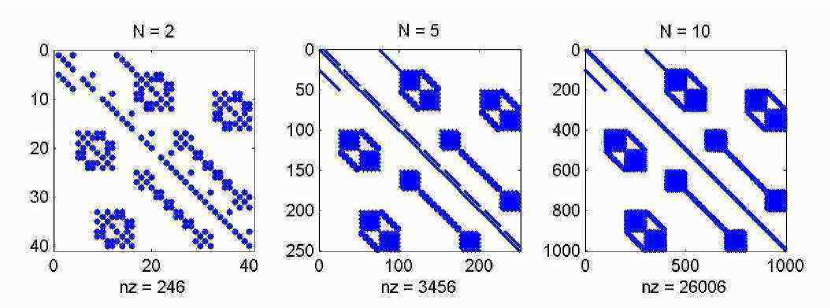
Refer to caption
Figure 3.5: Example of matrix representation of the Liouvillean for the TDQS. The Hilbert space of the harmonic oscillator has dimension respectively N=2,5,10𝑁2510N=2,5,10 (nz𝑛𝑧nz is the number of no-zero elements of the mtrix). The non-zero elements are represented by a blue dot. The exponentials of position operator present in the tunneling amplitudes make the Liouvillean non-sparse (large squares progressively emerging in the figures from left to right). For large N𝑁N the SVD is not viable and we use the Arnoldi iteration scheme to find the null space of the Liouvillean.

Chapter 4 Wigner function distribution

The shuttle dynamics has, especially in the single dot device, an appealing simple classical interpretation and one can say that the name itself of “shuttle” suggests the idea of sequential and periodical loading, mechanical transport and unloading of electrons between a source and a drain lead. Semiclassical models typically treat the mechanical degree of freedom classically combined with incoherent sequential tunneling of electrons between leads and oscillating dot [1, 2, 3, 4, 5]. Motivated by the small size of the oscillations of a nanoscale shuttle, and thus by the possibility to observe signatures of quantum dynamics of the mechanical degree of freedom, we decided, following the suggestion of Armour and MacKinnon [7], to explore the model with a quantized oscillator. Nevertheless we also wanted to keep as much as possible the intuitive classical picture and to handle the quantum-classical correspondence. The Wigner function distribution seemed to us a good answer to all these requirements. It allows a clear visualization of the numerical results obtained within the framework of the GME and it shows in its equation of motion (the Klein-Kramers equation) an explicit quantum-classical correspondence (expansion in powers of Planck-constant-over-2-pi\hbar) [34].

4.1 A quantum phase-space distribution

The concept of a probability distribution in phase space is problematic in quantum mechanics due to the uncertainty principle. It is not clear for example the meaning of the probability that a particle has a well defined position and momentum at a certain time and thus it seems difficult to define a probability distribution for such “non-observable events”. Nevertheless one can demonstrate that it is possible to associate with a state defined by a density operator ρ(t)𝜌𝑡\rho(t) a unique function P(q,p,t)𝑃𝑞𝑝𝑡P(q,p,t) on the phase space (q,p)×[t0,)𝑞𝑝subscript𝑡0(q,p)\times[t_{0},\infty) that satisfies some desirable properties. We list the required properties as stated by Hillary et al. in the review “Distribution functions in Physics: fundamentals” [34]:

  1. 1.

    P(q,p,t)𝑃𝑞𝑝𝑡P(q,p,t) should be real;

  2. 2.

    P(q,p,t)𝑃𝑞𝑝𝑡P(q,p,t) should reduce to a probability distribution once the conjugate variable is integrated:

    𝑑pP(q,p,t)=q|ρ(t)|q𝑑qP(q,p,t)=p|ρ(t)|pdifferential-d𝑝𝑃𝑞𝑝𝑡quantum-operator-product𝑞𝜌𝑡𝑞differential-d𝑞𝑃𝑞𝑝𝑡quantum-operator-product𝑝𝜌𝑡𝑝\begin{split}&\int dp\,P(q,p,t)=\langle q|\rho(t)|q\rangle\\ &\int dq\,P(q,p,t)=\langle p|\rho(t)|p\rangle\\ \end{split} (4.1)

    and thus P(q,p)𝑃𝑞𝑝P(q,p) is normalized

    𝑑p𝑑qP(q,p,t)=1differential-d𝑝differential-d𝑞𝑃𝑞𝑝𝑡1\int dp\int dq\,P(q,p,t)=1 (4.2)
  3. 3.

    P(q,p,t)𝑃𝑞𝑝𝑡P(q,p,t) should be Galilei invariant;

  4. 4.

    P(q,p,t)𝑃𝑞𝑝𝑡P(q,p,t) should be invariant under space and time reflection;

  5. 5.

    In the force free case P(q,p,t)𝑃𝑞𝑝𝑡P(q,p,t) should obey the classical equation of motion:

    Pt=pmPq𝑃𝑡𝑝𝑚𝑃𝑞\frac{\partial P}{\partial t}=-\frac{p}{m}\frac{\partial P}{\partial q} (4.3)
  6. 6.

    If P1(q,p,t)subscript𝑃1𝑞𝑝𝑡P_{1}(q,p,t) and P2(q,p,t)subscript𝑃2𝑞𝑝𝑡P_{2}(q,p,t) are the distributions corresponding to the states ρ1(t)subscript𝜌1𝑡\rho_{1}(t) and ρ2(t)subscript𝜌2𝑡\rho_{2}(t) the following relation should hold:

    𝑑qq|ρ1ρ2|q=2π𝑑q𝑑pP1(q,p,t)P2(q,p,t)differential-d𝑞quantum-operator-product𝑞subscript𝜌1subscript𝜌2𝑞2𝜋Planck-constant-over-2-pidifferential-d𝑞differential-d𝑝subscript𝑃1𝑞𝑝𝑡subscript𝑃2𝑞𝑝𝑡\int dq\langle q|\rho_{1}\rho_{2}|q\rangle=2\pi\hbar\int dq\int dp\,P_{1}(q,p,t)P_{2}(q,p,t) (4.4)

Condition 6 is a requirement that comes from quantum mechanical considerations as can be seen from the following consequences. Assume ρ1=ρ2=ρsubscript𝜌1subscript𝜌2𝜌\rho_{1}=\rho_{2}=\rho being statistical mixtures of pure states ραsubscript𝜌𝛼\rho_{\alpha} with weights wαsubscript𝑤𝛼w_{\alpha}

ρ=αwαρα𝜌subscript𝛼subscript𝑤𝛼subscript𝜌𝛼\rho=\sum_{\alpha}w_{\alpha}\rho_{\alpha} (4.5)

and P(q,p,t)𝑃𝑞𝑝𝑡P(q,p,t) the associated distribution, then from condition 6 we get

𝑑q𝑑p[P(q,p,t)]2=αwα22πdifferential-d𝑞differential-d𝑝superscriptdelimited-[]𝑃𝑞𝑝𝑡2subscript𝛼superscriptsubscript𝑤𝛼22𝜋Planck-constant-over-2-pi\int dq\int dp[P(q,p,t)]^{2}=\frac{\sum_{\alpha}w_{\alpha}^{2}}{2\pi\hbar} (4.6)

This relation is discarding any too peacked distribution. In particular the classical distribution P(q,p,t)=δ(qq0(t))δ(pp0(t))𝑃𝑞𝑝𝑡𝛿𝑞subscript𝑞0𝑡𝛿𝑝subscript𝑝0𝑡P(q,p,t)=\delta(q-q_{0}(t))\delta(p-p_{0}(t)) does not fulfill condition 6. If we assume now that ρ1subscript𝜌1\rho_{1} and ρ2subscript𝜌2\rho_{2} are pure states associated with orthogonal vectors, then:

𝑑q𝑑pP1(q,p,t)P2(q,p,t)=0differential-d𝑞differential-d𝑝subscript𝑃1𝑞𝑝𝑡subscript𝑃2𝑞𝑝𝑡0\int dq\int dpP_{1}(q,p,t)P_{2}(q,p,t)=0 (4.7)

which implies that the two distributions are not positive everywhere. For this reason the distribution we are axiomatically constructing will take the name of quasi-probability distribution.

The distribution function that satisfy properties (1-5) or (1-4 and 6) exists unique [35], is defined as

W(q,p,t)=12π+𝑑ξqξ2|ρ(t)|q+ξ2exp(ipξ)𝑊𝑞𝑝𝑡12𝜋Planck-constant-over-2-pisuperscriptsubscriptdifferential-d𝜉quantum-operator-product𝑞𝜉2𝜌𝑡𝑞𝜉2𝑖𝑝𝜉Planck-constant-over-2-piW(q,p,t)=\frac{1}{2\pi\hbar}\int_{-\infty}^{+\infty}\!\!\!d\xi\left\langle q-\frac{\xi}{2}\right|\rho(t)\left|q+\frac{\xi}{2}\right\rangle\exp\left(\frac{ip\xi}{\hbar}\right) (4.8)

and is commonly called Wigner distribution. The parallel with classical mechanics can be pushed even further associating to every observable on the Hilbert space the corresponding Wigner function:

A(q,p)=+𝑑ξqξ2|A|q+ξ2exp(ipξ)𝐴𝑞𝑝superscriptsubscriptdifferential-d𝜉quantum-operator-product𝑞𝜉2𝐴𝑞𝜉2𝑖𝑝𝜉Planck-constant-over-2-piA(q,p)=\int_{-\infty}^{+\infty}\!\!\!d\xi\left\langle q-\frac{\xi}{2}\right|A\left|q+\frac{\xi}{2}\right\rangle\exp\left(\frac{ip\xi}{\hbar}\right) (4.9)

Two important relations can be derived from the definitions (4.8) and (4.9).

  1. 1.

    The trace of an operator in proportional to the integral on the phase space of its corresponding Wigner function:

    TrA=12π𝑑q𝑑pA(q,p)Tr𝐴12𝜋Planck-constant-over-2-pidifferential-d𝑞differential-d𝑝𝐴𝑞𝑝{\rm Tr}A=\frac{1}{2\pi\hbar}\int dq\int dp\,A(q,p) (4.10)
  2. 2.

    Given two operators A𝐴A and B𝐵B and the associate Wigner functions A(q,p)𝐴𝑞𝑝A(q,p) and B(q,p)𝐵𝑞𝑝B(q,p), the Wigner function associated to the product of the two operators F=AB𝐹𝐴𝐵F=AB reads [35]111This relation was first derived by Groenewold in 1946 in the context of an rigorous mathematical correspondence between commutator and poisson bracket in the limit 0Planck-constant-over-2-pi0\hbar\to 0.:

F(q,p)=A(q,p)exp(Λ2i)B(q,p)𝐹𝑞𝑝𝐴𝑞𝑝Planck-constant-over-2-piΛ2𝑖𝐵𝑞𝑝F(q,p)=A(q,p)\exp\left(\frac{\hbar\Lambda}{2i}\right)B(q,p) (4.11)

where ΛΛ\Lambda is the differential operator:

Λ=pqqpΛ𝑝𝑞𝑞𝑝\Lambda=\frac{\overleftarrow{\partial}}{\partial p}\frac{\overrightarrow{\partial}}{\partial q}-\frac{\overleftarrow{\partial}}{\partial q}\frac{\overrightarrow{\partial}}{\partial p} (4.12)

The arrows indicate in which direction the derivative should be taken. A better insight in the expression (4.11) is given by the expansion of the exponential. Up to the first two terms it reads:

F(q,p)=A(q,p)B(q,p)+2i(ApBqAqBp)+(2i)2(2Ap22Bq222Apq2Bqp+2Aq22Bp2)+(2i)3𝐹𝑞𝑝𝐴𝑞𝑝𝐵𝑞𝑝Planck-constant-over-2-pi2𝑖𝐴𝑝𝐵𝑞𝐴𝑞𝐵𝑝superscriptPlanck-constant-over-2-pi2𝑖2superscript2𝐴superscript𝑝2superscript2𝐵superscript𝑞22superscript2𝐴𝑝𝑞superscript2𝐵𝑞𝑝superscript2𝐴superscript𝑞2superscript2𝐵superscript𝑝2superscriptPlanck-constant-over-2-pi2𝑖3\begin{split}F(q,p)=&A(q,p)B(q,p)\\ +&\frac{\hbar}{2i}\left(\frac{\partial A}{\partial p}\frac{\partial B}{\partial q}-\frac{\partial A}{\partial q}\frac{\partial B}{\partial p}\right)\\ +&\left(\frac{\hbar}{2i}\right)^{2}\left(\frac{\partial^{2}A}{\partial p^{2}}\frac{\partial^{2}B}{\partial q^{2}}-2\frac{\partial^{2}A}{\partial p\partial q}\frac{\partial^{2}B}{\partial q\partial p}+\frac{\partial^{2}A}{\partial q^{2}}\frac{\partial^{2}B}{\partial p^{2}}\right)\\ +&\left(\frac{\hbar}{2i}\right)^{3}\ldots\end{split} (4.13)

The expansion shows the power of the formalism to treat the quantum-classical correspondence: given a length, a mass, and a time scale for the system we can rescale the coordinates and the expansion will appear as an expansion in /SsysPlanck-constant-over-2-pisubscript𝑆sys\hbar/S_{\rm sys} where Ssyssubscript𝑆sysS_{\rm sys} is the typical action of the system. Classical systems have a large action Ssysmuch-greater-thansubscript𝑆𝑠𝑦𝑠Planck-constant-over-2-piS_{sys}\gg\hbar and only the first term in the expansion is relevant. In the opposite limit Ssyssubscript𝑆𝑠𝑦𝑠Planck-constant-over-2-piS_{sys}\approx\hbar the full expansion should be considered. We have now the tools to translate into the Wigner formalism the expression for the expectation value of an operator: We start from the definitions:

A(t)Tr{ρ(t)A}=𝑑q𝑑pW(q,p,t)exp(Λ2i)A(q,p)delimited-⟨⟩𝐴𝑡Tr𝜌𝑡𝐴differential-d𝑞differential-d𝑝𝑊𝑞𝑝𝑡Planck-constant-over-2-piΛ2𝑖𝐴𝑞𝑝\langle A(t)\rangle\equiv{\rm Tr}\{\rho(t)A\}=\int dq\int dp\,W(q,p,t)\exp\left(\frac{\hbar\Lambda}{2i}\right)A(q,p) (4.14)

Inserting the expansion in Planck-constant-over-2-pi\hbar of the exponential and using the regularity of the Wigner distribution at infinity we obtain the “classical” result:

A(t)=𝑑q𝑑pW(q,p,t)A(q,p)delimited-⟨⟩𝐴𝑡differential-d𝑞differential-d𝑝𝑊𝑞𝑝𝑡𝐴𝑞𝑝\langle A(t)\rangle=\int dq\int dp\,W(q,p,t)A(q,p) (4.15)

A second important consequence of the Groenewold equation (4.11) is the quantum-classical correspondence for the dynamics of the distribution function W(q,p,t)𝑊𝑞𝑝𝑡W(q,p,t). In the Wigner formalism the equation of Liouville-von Neumann reads:

Wt=i[Hexp(Λ2i)WWexp(Λ2i)H]𝑊𝑡𝑖Planck-constant-over-2-pidelimited-[]𝐻Planck-constant-over-2-piΛ2𝑖𝑊𝑊Planck-constant-over-2-piΛ2𝑖𝐻\frac{\partial W}{\partial t}=-\frac{i}{\hbar}\left[H\exp\left(\frac{\hbar\Lambda}{2i}\right)W-W\exp\left(\frac{\hbar\Lambda}{2i}\right)H\right] (4.16)

where HH(q,p)𝐻𝐻𝑞𝑝H\equiv H(q,p) is the Wigner function associated with the Hamiltonian for the system. Due to the fact that the differential operator ΛΛ\Lambda is odd with respect of the exchange of the two functions on which it is acting only odd powers of the expansion in /SsysPlanck-constant-over-2-pisubscript𝑆sys\hbar/S_{\rm sys} survive in (4.16). In the limit /Ssys0Planck-constant-over-2-pisubscript𝑆sys0\hbar/S_{\rm sys}\to 0 we get the classical Liouville equation:

Wct={H,Wc}Psuperscript𝑊𝑐𝑡subscript𝐻superscript𝑊𝑐𝑃\frac{\partial W^{c}}{\partial t}=\{H,W^{c}\}_{P} (4.17)

where {,}Pqppq=Λ\{,\}_{P}\equiv\frac{\overleftarrow{\partial}}{\partial q}\frac{\overrightarrow{\partial}}{\partial p}-\frac{\overleftarrow{\partial}}{\partial p}\frac{\overrightarrow{\partial}}{\partial q}=-\Lambda are the Poisson brackets and the superscript c𝑐c indicates the classical limit for the Wigner distribution222As can be seen from this derivation, in the framework of the Wigner distribution the quantum-classical limit attributed to Dirac i[,]{,}P-\frac{i}{\hbar}[,]\to\{,\}_{P} for 0Planck-constant-over-2-pi0\hbar\to 0 acquires a precise mathematical meaning..

4.2 Klein-Kramers equations for the SDQS

With the knowledge acquired in the previous section we will now concentrate on the translation in the Wigner formalism of the GME for shuttle devices that we derived in the previous chapter. We concentrate only on the SDQS first because the technique is completely illustrated in this simpler case and also because contrary to the single dot device for the TDQS we will use the Wigner distribution only as a visualization tool. In the derivation of the GME for the single dot device (see §3.4.1) we identified three components of the Liouvillean super-operator:

=coh+driv+dampsubscriptcohsubscriptdrivsubscriptdamp\mathcal{L}=\mathcal{L}_{\rm coh}+\mathcal{L}_{\rm driv}+\mathcal{L}_{\rm damp} (4.18)

distinguishing the coherent contribution that describes the evolution of the system without the electrical and mechanical baths from a driving contribution where the coupling to the leads is inserted and a damping term that takes into account the interaction with the dissipative environment of the mechanical degree of freedom. We separately treat their translation into the Wigner formalism in the following sections.

4.2.1 Coherent Liouvillean

We start recalling explicitly the action of the coherent part of the Liouvillean on the two non-vanishing333For an explanation on the vanishing electrical coherencies σ01subscript𝜎01\sigma_{01} and σ10subscript𝜎10\sigma_{10} see §3.3.4. electrical components of the reduced density matrix (σ00subscript𝜎00\sigma_{00} and σ11subscript𝜎11\sigma_{11}):

coh(σ00σ11)=i([Hosc,σ00][Hoscex,σ11])subscriptcohsubscript𝜎00subscript𝜎11𝑖Planck-constant-over-2-pisubscript𝐻oscsubscript𝜎00subscript𝐻osc𝑒𝑥subscript𝜎11\mathcal{L}_{\rm coh}\left(\begin{array}[]{c}\sigma_{00}\\ \sigma_{11}\end{array}\right)=-\frac{i}{\hbar}\left(\begin{array}[]{c}{[H_{\rm osc},\sigma_{00}]}\\ {[H_{\rm osc}-e\mathcal{E}x,\sigma_{11}]}\end{array}\right) (4.19)

It is easy to verify from the definition (4.9) that for operators which are sum of functions of momentum or position operator only, the associated Winger functions coincide with the corresponding classical dynamical variables. For example the Wigner function of the oscillator Hamiltonian reads:

Hosc(q,p)=p22m+12mω2q2subscript𝐻osc𝑞𝑝superscript𝑝22𝑚12𝑚superscript𝜔2superscript𝑞2H_{\rm osc}(q,p)=\frac{p^{2}}{2m}+\frac{1}{2}m\omega^{2}q^{2} (4.20)

and analogously the electrostatic component becomes eq𝑒𝑞e\mathcal{E}q.

As already mentioned the commutator structure of the Liouville-von Neumann equation implies that only the odd components of the Planck-constant-over-2-pi\hbar expansion of the Groenewold operator exp(Λ/2i)Planck-constant-over-2-piΛ2𝑖\exp(\hbar\Lambda/2i) should be retained. Since the third order in the expansion contains already derivatives in q𝑞q and p𝑝p up to the third order, and the oscillator Hamiltonian is quadratic in q𝑞q and p𝑝p only the first order survives and the coherent part of the Liouvilliean acquires the classical form444This result is more general and resembles the Ehrenfest theorem for Hamiltonian up to second order in x and p. In that case one gets classical equations of motion for the expectation values xdelimited-⟨⟩𝑥\langle x\rangle and pdelimited-⟨⟩𝑝\langle p\rangle.:

coh(W00W11)=(mω2qW00ppmW00qmω2(qd)W11ppmW11q)subscriptcohsubscript𝑊00subscript𝑊11𝑚superscript𝜔2𝑞subscript𝑊00𝑝𝑝𝑚subscript𝑊00𝑞𝑚superscript𝜔2𝑞𝑑subscript𝑊11𝑝𝑝𝑚subscript𝑊11𝑞\mathcal{L}_{\rm coh}\left(\begin{array}[]{c}W_{00}\\ W_{11}\end{array}\right)=\left(\begin{array}[]{c}{m\omega^{2}q\frac{\partial W_{00}}{\partial p}-\frac{p}{m}\frac{\partial W_{00}}{\partial q}}\\ {m\omega^{2}(q-d)\frac{\partial W_{11}}{\partial p}-\frac{p}{m}\frac{\partial W_{11}}{\partial q}}\end{array}\right) (4.21)

where the displacement d=emω2𝑑𝑒𝑚superscript𝜔2d=\frac{e\mathcal{E}}{m\omega^{2}} is the equilibrium position of the oscillator subject to a constant force e𝑒e\mathcal{E} and we have introduced a Wigner distribution for each of the electrical states of the system. In this charge resolved Wigner functions one can read the probability density for the quantum dot to have a specific position and (average) momentum when in a specific electrical state. In this way we can monitor the correlation between charge and position (momentum) of the oscillating dot, important to discriminate the shuttling regime from other transport regimes.

4.2.2 Driving Liouvillean

The driving term of the Liouvillean for the SDQS is a rate equation somehow modified to take into account the operator form of the position-dependent rates:

driv(σ00σ11)=(ΓL2{e2x/λ,σ00}+ΓRex/λσ11ex/λΓR2{e2x/λ,σ11}+ΓLex/λσ00ex/λ)subscriptdrivsubscript𝜎00subscript𝜎11subscriptΓ𝐿2superscript𝑒2𝑥𝜆subscript𝜎00subscriptΓ𝑅superscript𝑒𝑥𝜆subscript𝜎11superscript𝑒𝑥𝜆subscriptΓ𝑅2superscript𝑒2𝑥𝜆subscript𝜎11subscriptΓ𝐿superscript𝑒𝑥𝜆subscript𝜎00superscript𝑒𝑥𝜆\mathcal{L}_{\rm driv}\left(\begin{array}[]{c}\sigma_{00}\\ \sigma_{11}\\ \end{array}\right)=\left(\begin{array}[]{c}-\frac{\Gamma_{L}}{2}\{e^{-2x/\lambda},\sigma_{00}\}+\Gamma_{R}e^{x/\lambda}\sigma_{11}e^{x/\lambda}\\ -\frac{\Gamma_{R}}{2}\{e^{2x/\lambda},\sigma_{11}\}+\Gamma_{L}e^{-x/\lambda}\sigma_{00}e^{-x/\lambda}\\ \end{array}\right) (4.22)

where {A,B}AB+BA𝐴𝐵𝐴𝐵𝐵𝐴\{A,B\}\equiv AB+BA is the anticommutator.

We calculate first the generic form of the symmetric component of the driving Liouvillian in the Wigner representation. It is easier in this case to start directly from the definition:

12π+𝑑ξqξ2|ΓL,Rex/λσii(t)ex/λ|q+ξ2exp(ipξ)=ΓL,Re2q/λ+𝑑ξqξ2|σii(t)|q+ξ2exp(ipξ)=ΓL,Re2q/λWii(q,p,t)12𝜋Planck-constant-over-2-pisuperscriptsubscriptdifferential-d𝜉quantum-operator-product𝑞𝜉2subscriptΓ𝐿𝑅superscript𝑒minus-or-plus𝑥𝜆subscript𝜎𝑖𝑖𝑡superscript𝑒minus-or-plus𝑥𝜆𝑞𝜉2𝑖𝑝𝜉Planck-constant-over-2-pisubscriptΓ𝐿𝑅superscript𝑒minus-or-plus2𝑞𝜆superscriptsubscriptdifferential-d𝜉quantum-operator-product𝑞𝜉2subscript𝜎𝑖𝑖𝑡𝑞𝜉2𝑖𝑝𝜉Planck-constant-over-2-pisubscriptΓ𝐿𝑅superscript𝑒minus-or-plus2𝑞𝜆subscript𝑊𝑖𝑖𝑞𝑝𝑡\begin{split}&\frac{1}{2\pi\hbar}\int_{-\infty}^{+\infty}\!\!\!d\xi\left\langle q-\frac{\xi}{2}\right|\Gamma_{L,R}e^{\mp x/\lambda}\sigma_{ii}(t)e^{\mp x/\lambda}\left|q+\frac{\xi}{2}\right\rangle\exp\left(\frac{ip\xi}{\hbar}\right)\\ =&\,\Gamma_{L,R}e^{\mp 2q/\lambda}\int_{-\infty}^{+\infty}\!\!\!d\xi\left\langle q-\frac{\xi}{2}\right|\sigma_{ii}(t)\left|q+\frac{\xi}{2}\right\rangle\exp\left(\frac{ip\xi}{\hbar}\right)\\ =&\Gamma_{L,R}e^{\mp 2q/\lambda}W_{ii}(q,p,t)\end{split} (4.23)

where i=0,1𝑖01i=0,1 in accordance with the sign of the exponential respectively ,+-,+ and the subscript L,R𝐿𝑅L,R in the tunneling rate ΓΓ\Gamma. Only the classical component contributes to this term since the Wigner representation is just the product of the three Wigner functions.

Quantum correction are present instead in the anticommutator component of the driving Liouvillean. Again we calculate the generic form :

12π+𝑑ξqξ2|ΓL,R2{e2x/λ,σii(t)}|q+ξ2exp(ipξ)=ΓL,R2[e2q/λexp(Λ2i)Wii(q,p,t)+Wii(q,p,t)exp(Λ2i)e2q/λ]=ΓL,Re2q/λn=01(2n)!(Λ2i)2nWii(q,p,t)=ΓL,Re2q/λn=0(1)n(2n)!(λ)2n2np2nWii(q,p,t)12𝜋Planck-constant-over-2-pisuperscriptsubscriptdifferential-d𝜉quantum-operator-product𝑞𝜉2subscriptΓ𝐿𝑅2superscript𝑒minus-or-plus2𝑥𝜆subscript𝜎𝑖𝑖𝑡𝑞𝜉2𝑖𝑝𝜉Planck-constant-over-2-pisubscriptΓ𝐿𝑅2delimited-[]superscript𝑒minus-or-plus2𝑞𝜆Planck-constant-over-2-piΛ2𝑖subscript𝑊𝑖𝑖𝑞𝑝𝑡subscript𝑊𝑖𝑖𝑞𝑝𝑡Planck-constant-over-2-piΛ2𝑖superscript𝑒minus-or-plus2𝑞𝜆subscriptΓ𝐿𝑅superscript𝑒minus-or-plus2𝑞𝜆superscriptsubscript𝑛012𝑛superscriptPlanck-constant-over-2-piΛ2𝑖2𝑛subscript𝑊𝑖𝑖𝑞𝑝𝑡subscriptΓ𝐿𝑅superscript𝑒minus-or-plus2𝑞𝜆superscriptsubscript𝑛0superscript1𝑛2𝑛superscriptPlanck-constant-over-2-pi𝜆2𝑛superscript2𝑛superscript𝑝2𝑛subscript𝑊𝑖𝑖𝑞𝑝𝑡\begin{split}&-\frac{1}{2\pi\hbar}\int_{-\infty}^{+\infty}\!\!\!d\xi\left\langle q-\frac{\xi}{2}\right|\frac{\Gamma_{L,R}}{2}\{e^{\mp 2x/\lambda},\sigma_{ii}(t)\}\left|q+\frac{\xi}{2}\right\rangle\exp\left(\frac{ip\xi}{\hbar}\right)\\ =&\,-\frac{\Gamma_{L,R}}{2}\left[e^{\mp 2q/\lambda}\exp\left(\frac{\hbar\Lambda}{2i}\right)W_{ii}(q,p,t)+W_{ii}(q,p,t)\exp\left(\frac{\hbar\Lambda}{2i}\right)e^{\mp 2q/\lambda}\right]\\ =&-\Gamma_{L,R}e^{\mp 2q/\lambda}\sum_{n=0}^{\infty}\frac{1}{(2n)!}\left(\frac{\hbar\Lambda}{2i}\right)^{2n}W_{ii}(q,p,t)\\ =&-\Gamma_{L,R}e^{\mp 2q/\lambda}\sum_{n=0}^{\infty}\frac{(-1)^{n}}{(2n)!}\left(\frac{\hbar}{\lambda}\right)^{2n}\frac{\partial^{2n}}{\partial p^{2n}}W_{ii}(q,p,t)\end{split} (4.24)

where because of the symmetry of the anticommutator only even powers of the Groenewold operator give non vanishing contributions (line 2 to 3 in (4.24) ) and they are equal for both terms of the anticommutator. In the last line we appreciate the control parameter for the quantum-classical correspondence. Especially in the shuttling regime the typical length, mass and time scales of the system are the tunneling length λ𝜆\lambda and the harmonic oscillator mass m𝑚m and inverse frequency 1/ω1𝜔1/\omega. Rescaling the phase space coordinates to the adimensional X=q/λ𝑋𝑞𝜆X=q/\lambda and P=p/(mωλ)𝑃𝑝𝑚𝜔𝜆P=p/(m\omega\lambda) we obtain the expansion parameter:

mωλ2=2(Δxzλ)2Planck-constant-over-2-pi𝑚𝜔superscript𝜆22superscriptΔsubscript𝑥𝑧𝜆2\frac{\hbar}{m\omega\lambda^{2}}=2\left(\frac{\Delta x_{z}}{\lambda}\right)^{2} (4.25)

that is the ratio between the zero point fluctuation of the oscillator position (ΔxzΔsubscript𝑥𝑧\Delta x_{z}) and the tunneling length (λ𝜆\lambda). The bigger λ𝜆\lambda the more classical is the behavior of the harmonic oscillator.

All together the driving Liouvillean in the Wigner representation takes the form:

driv(W00W11)=(ΓRe2q/λW11ΓLe2q/λn=0(1)n(2n)!(λ)2n2np2nW00ΓLe2q/λW00ΓRe2q/λn=0(1)n(2n)!(λ)2n2np2nW11)subscriptdrivsubscript𝑊00subscript𝑊11subscriptΓ𝑅superscript𝑒2𝑞𝜆subscript𝑊11subscriptΓ𝐿superscript𝑒2𝑞𝜆superscriptsubscript𝑛0superscript1𝑛2𝑛superscriptPlanck-constant-over-2-pi𝜆2𝑛superscript2𝑛superscript𝑝2𝑛subscript𝑊00subscriptΓ𝐿superscript𝑒2𝑞𝜆subscript𝑊00subscriptΓ𝑅superscript𝑒2𝑞𝜆superscriptsubscript𝑛0superscript1𝑛2𝑛superscriptPlanck-constant-over-2-pi𝜆2𝑛superscript2𝑛superscript𝑝2𝑛subscript𝑊11\mathcal{L}_{\rm driv}\left(\begin{array}[]{c}W_{00}\\ W_{11}\end{array}\right)=\left(\begin{array}[]{c}{\Gamma_{R}e^{2q/\lambda}W_{11}-\Gamma_{L}e^{-2q/\lambda}\sum_{n=0}^{\infty}\frac{(-1)^{n}}{(2n)!}\left(\frac{\hbar}{\lambda}\right)^{2n}\frac{\partial^{2n}}{\partial p^{2n}}W_{00}}\\ {\Gamma_{L}e^{-2q/\lambda}W_{00}-\Gamma_{R}e^{2q/\lambda}\sum_{n=0}^{\infty}\frac{(-1)^{n}}{(2n)!}\left(\frac{\hbar}{\lambda}\right)^{2n}\frac{\partial^{2n}}{\partial p^{2n}}W_{11}}\end{array}\right) (4.26)

4.2.3 Damping Liouvillean

The damping Liouvillean is identical for the two electrical components of the reduced density matrix and we give a unified derivation of the corresponding Wigner formulation. In terms of density matrices it reads:

damp(σ)=iγ2[x,{p,σ}]γmω2(2nB+1)[x,[x,σ]]subscriptdamp𝜎𝑖𝛾2Planck-constant-over-2-pi𝑥𝑝𝜎𝛾𝑚𝜔2Planck-constant-over-2-pi2subscript𝑛𝐵1𝑥𝑥𝜎\mathcal{L}_{\rm damp}(\sigma)=-\frac{i\gamma}{2\hbar}[x,\{p,\sigma\}]-\frac{\gamma m\omega}{2\hbar}(2n_{B}+1)[x,[x,\sigma]] (4.27)

Once again we apply the Groenewold modified product555The product of three operator can be handled easily since one can split the product in two parts and the property (AB)C=A(BC)𝐴𝐵𝐶𝐴𝐵𝐶(A*B)*C=A*(B*C) holds, where we have indicated with * the Groenewold modified product. (4.11) to obtain the Wigner formulation. Since the damping Liouvillean is quadratic in the operators x𝑥x and p𝑝p we expect only the first two terms of the expansion in the operator ΛΛ\Lambda to contribute.

dampW=γppW+γmω(nB+12)2p2Wsubscriptdamp𝑊𝛾𝑝𝑝𝑊𝛾𝑚Planck-constant-over-2-pi𝜔subscript𝑛𝐵12superscript2superscript𝑝2𝑊\mathcal{L}_{\rm damp}W=\gamma\frac{\partial}{\partial p}pW+\gamma m\hbar\omega\left(n_{B}+\frac{1}{2}\right)\frac{\partial^{2}}{\partial p^{2}}W (4.28)

The term of first order in the derivative is called damping term while the second diffusion term. One way to understand the meaning of this names is to derive this equation for the distribution function starting from the corresponding Langevin equations describing the brownian motion of a particle in an harmonic potential:

x˙=pmp˙=mω2xγp+ξ(t)˙𝑥𝑝𝑚˙𝑝𝑚superscript𝜔2𝑥𝛾𝑝𝜉𝑡\begin{split}\dot{x}&=\frac{p}{m}\\ \dot{p}&=-m\omega^{2}x-\gamma p+\xi(t)\end{split} (4.29)

The first term in the RHS of equation (4.28) is related to the velocity dependent friction (γp𝛾𝑝-\gamma p) while the second comes from the stochastic force ξ(t)𝜉𝑡\xi(t). The analogy with classical brownian motion can be pushed even further considering the rescaling:

X=x,P=pmωformulae-sequence𝑋𝑥𝑃𝑝𝑚𝜔X=\frac{x}{\ell},\qquad P=\frac{p}{m\omega\ell} (4.30)

where =2mω(2nB+1)Planck-constant-over-2-pi2𝑚𝜔2subscript𝑛𝐵1\ell=\sqrt{\frac{\hbar}{2m\omega}(2n_{B}+1)}. The damping Liouvillian in terms of the rescaled variables reads:

damp(W)=γP(P+P)Wsubscriptdamp𝑊𝛾𝑃𝑃𝑃𝑊\mathcal{L}_{\rm damp}(W)=\gamma\frac{\partial}{\partial P}\left(P+\frac{\partial}{\partial P}\right)\,W (4.31)

and only the scaling666Quantum contribution (e.g regions of negative distribution W(q,p,t)<0𝑊𝑞𝑝𝑡0W(q,p,t)<0) could be contained in the coherence of the initial condition. These will anyway be decohered by the damping Liouvillean itself. distinguishes the quantum from the classical description While in the low temperature limit 2nB1much-less-than2subscript𝑛𝐵12n_{B}\ll 1 and the length scale \ell tends to the oscillator zero point fluctuation ΔxzΔsubscript𝑥𝑧\Delta x_{z}, in the high temperature limit Planck-constant-over-2-pi\hbar drops out from the equations and \ell is given by the the thermal length λth=kBTmω2subscript𝜆𝑡subscript𝑘𝐵𝑇𝑚superscript𝜔2\lambda_{th}=\sqrt{\frac{k_{B}T}{m\omega^{2}}}.

Finally we collect the results of the previous sections and write the equation of motion for the SDQS in the Wigner function formulation:

W00t=subscript𝑊00𝑡absent\displaystyle\frac{\partial W_{00}}{\partial t}= [mω2qppmq+γpp+γmω(nB+12)2p2]W00delimited-[]𝑚superscript𝜔2𝑞𝑝𝑝𝑚𝑞𝛾𝑝𝑝𝛾𝑚Planck-constant-over-2-pi𝜔subscript𝑛𝐵12superscript2superscript𝑝2subscript𝑊00\displaystyle\!\!\!\left[m\omega^{2}q\frac{\partial}{\partial p}-\frac{p}{m}\frac{\partial}{\partial q}+\gamma\frac{\partial}{\partial p}p+\gamma m\hbar\omega\left(n_{B}+\frac{1}{2}\right)\frac{\partial^{2}}{\partial p^{2}}\right]W_{00}
+ΓRe2q/λW11ΓLe2q/λn=0(1)n(2n)!(λ)2n2nW00p2nsubscriptΓ𝑅superscript𝑒2𝑞𝜆subscript𝑊11subscriptΓ𝐿superscript𝑒2𝑞𝜆superscriptsubscript𝑛0superscript1𝑛2𝑛superscriptPlanck-constant-over-2-pi𝜆2𝑛superscript2𝑛subscript𝑊00superscript𝑝2𝑛\displaystyle\!\!\!+\Gamma_{R}e^{2q/\lambda}W_{11}-\Gamma_{L}e^{-2q/\lambda}\sum_{n=0}^{\infty}\frac{(-1)^{n}}{(2n)!}\left(\frac{\hbar}{\lambda}\right)^{2n}\frac{\partial^{2n}W_{00}}{\partial p^{2n}}
W11t=subscript𝑊11𝑡absent\displaystyle\frac{\partial W_{11}}{\partial t}= [mω2(qd)ppmq+γpp+γmω(nB+12)2p2]W11delimited-[]𝑚superscript𝜔2𝑞𝑑𝑝𝑝𝑚𝑞𝛾𝑝𝑝𝛾𝑚Planck-constant-over-2-pi𝜔subscript𝑛𝐵12superscript2superscript𝑝2subscript𝑊11\displaystyle\!\!\!\left[m\omega^{2}(q-d)\frac{\partial}{\partial p}-\frac{p}{m}\frac{\partial}{\partial q}+\gamma\frac{\partial}{\partial p}p+\gamma m\hbar\omega\left(n_{B}+\frac{1}{2}\right)\frac{\partial^{2}}{\partial p^{2}}\right]W_{11}
+ΓLe2q/λW00ΓRe2q/λn=0(1)n(2n)!(λ)2n2nW11p2nsubscriptΓ𝐿superscript𝑒2𝑞𝜆subscript𝑊00subscriptΓ𝑅superscript𝑒2𝑞𝜆superscriptsubscript𝑛0superscript1𝑛2𝑛superscriptPlanck-constant-over-2-pi𝜆2𝑛superscript2𝑛subscript𝑊11superscript𝑝2𝑛\displaystyle\!\!\!+\Gamma_{L}e^{-2q/\lambda}W_{00}-\Gamma_{R}e^{2q/\lambda}\sum_{n=0}^{\infty}\frac{(-1)^{n}}{(2n)!}\left(\frac{\hbar}{\lambda}\right)^{2n}\frac{\partial^{2n}W_{11}}{\partial p^{2n}}
(4.32)
Refer to caption
Figure 4.1: Example of 3-D visualization of the stationary solution of the Klein-Kramers equations for the SDQS. The surface represents the quasi-probability distribution of the empty dot W00stat(q,p)subscriptsuperscript𝑊𝑠𝑡𝑎𝑡00𝑞𝑝W^{stat}_{00}(q,p). Coordinate and momentum are expressed in adimensional units: X=q/x0𝑋𝑞subscript𝑥0X=q/x_{0} and P=px0/𝑃𝑝subscript𝑥0Planck-constant-over-2-piP=px_{0}/\hbar, where x0=/(mω)subscript𝑥0Planck-constant-over-2-pi𝑚𝜔x_{0}=\sqrt{\hbar/(m\omega)}. The distribution shows two distinct features. The probability is high near the origin of the phase space and represents the oscillator in the ground state. The other structure corresponds to the part of the limit cycle drawn by the empty dot in the shuttling regime.

Chapter 5 Investigation tools

The dynamics of the shuttling devices or at least of the simplified models for them that we consider, is all contained in the GMEs for the reduced density matrices (3.120) and (3.131) or in the corresponding Klein-Kramers equations for the Wigner distributions (e.g. equation (4.32) for the SDQS). The coupling to the continuum of states in the electrical and mechanical baths introduces irreversibility in the system and its statistical properties (represented by the reduced density matrix or Wigner distribution) tend to a stationary limit. This does not mean that the system itself is in a static condition. In particular an electric current sustained by the bias always flows through the device driving the movable dot into a variety of different dynamical regimes. In order to analyze the properties of these different operating conditions of the electronic shuttles we use three investigation tools. We study the phase space distribution functions associated with the stationary solution of the GME, the corresponding current and the current-noise, taking as control parameters the damping rate of the mechanical degree of freedom, or the gate voltage of the different dots, or the injection and ejection rates. Through the phase-space analysis or the current and noise calculation we gain somehow complementary information about the system. These approaches are described in detail in the next three sections.

5.1 Phase space distributions: dots, rings and bananas

The phase space analysis of the shuttle dynamics is based on the Wigner representation of the stationary solution of the GME:

Wijstat(q,p)=12π+𝑑ξqξ2|σijstat|q+ξ2exp(ipξ)superscriptsubscript𝑊𝑖𝑗stat𝑞𝑝12𝜋Planck-constant-over-2-pisuperscriptsubscriptdifferential-d𝜉quantum-operator-product𝑞𝜉2superscriptsubscript𝜎𝑖𝑗stat𝑞𝜉2𝑖𝑝𝜉Planck-constant-over-2-piW_{ij}^{\rm stat}(q,p)=\frac{1}{2\pi\hbar}\int_{-\infty}^{+\infty}\!\!\!d\xi\left\langle q-\frac{\xi}{2}\right|\sigma_{ij}^{\rm stat}\left|q+\frac{\xi}{2}\right\rangle\exp\left(\frac{ip\xi}{\hbar}\right) (5.1)

where the subscript ij𝑖𝑗ij indicates the electrical state that we are considering. Since typically we are not interested in coherencies111The probabilistic interpretation of the Wigner distribution would not be acceptable for electronic coherencies. between electronic states we set i=j𝑖𝑗i=j and the resulting Wigner distribution represents the joint probability for the system to be in the specific mechanical state (q,p)𝑞𝑝(q,p) and electrical state i𝑖i. The total Wigner distribution

Wtotstat(q,p)=iWiistat(q,p)subscriptsuperscript𝑊stattot𝑞𝑝subscript𝑖subscriptsuperscript𝑊stat𝑖𝑖𝑞𝑝W^{\rm stat}_{\rm tot}(q,p)=\sum_{i}W^{\rm stat}_{ii}(q,p) (5.2)

where the sum is extended to all the electrical states of the system, gives information about the mechanical state independently from the electronic state of the device.

5.1.1 Shuttling instability

For the SDQS we analyze first the behavior of the Wigner distribution as a function of the mechanical damping. The mechanical dynamics shows a typical feature qualitatively independent from the other parameters of the model. At high damping rates the total Wigner distribution is concentrated around the origin of the phase space and represents the harmonic oscillator in the ground state. While reducing the mechanical damping a ring progressively develops and the central “dot” eventually disappears (Fig. 5.1). We interpret the ring as a smeared limit cycle trajectory: by reducing the damping the equilibrium position becomes unstable and a stable limit cycle develops. The threshold for this transition is given by the effective tunneling rates of the electrons222A more precise definition of this electronic time can be found the next chapter..

This interpretation is represented in the following picture: every time an electron jumps on the movable grain the latter is subject to the electrostatic force e𝑒e\mathcal{E} that accelerates it towards the right. Energy is pumped into the mechanical system and the dot starts to oscillate. If the damping is high compared to the tunneling rates the oscillator dissipates this energy into the environment before the next tunneling event: on average the dot remains in its ground state. On the contrary for very small damping the relaxation time of the oscillator is long and multiple “forcing events” happen before the relaxation takes place. This continuously drives the oscillator far from equilibrium and a stationary state is reached only when the energy pumped per cycle into the system is dissipated during the same cycle in the environment.

It is not difficult to realize that, like for a macroscopic swing, in order to sustain the motion one needs coordination between forcing (here related to the electrical dynamics) and oscillations. This coordination is revealed by the charge resolved Wigner distributions W00subscript𝑊00W_{00} and W11subscript𝑊11W_{11}. The ring that appears in the total distribution is asymmetrically shared by the empty and charged-dot distributions (Fig. 5.1).
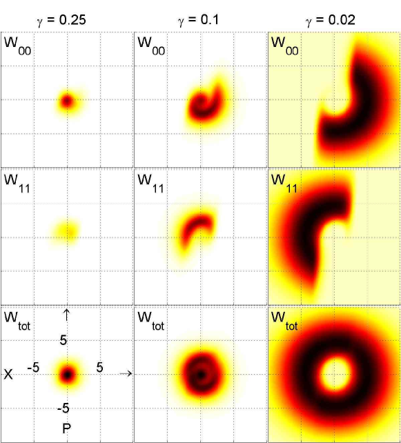
Refer to caption
Figure 5.1: Phase space picture of the tunneling-to-shuttling crossover. The respective rows show the Wigner distribution functions for the discharged (W00subscript𝑊00W_{00}), charged (W11subscript𝑊11W_{11}) and sum (Wtotsubscript𝑊totW_{\rm tot}) states of the oscillator in the phase space (horizontal axis–coordinate in units of x0=/(ω)subscript𝑥0Planck-constant-over-2-piPlanck-constant-over-2-pi𝜔x_{0}=\sqrt{\hbar/(\hbar\omega)}, vertical axis – momentum in /x0Planck-constant-over-2-pisubscript𝑥0\hbar/x_{0}). The values of the parameters are: λ=x0𝜆subscript𝑥0\lambda=x_{0}, T=0𝑇0T=0, d=0.5x0𝑑0.5subscript𝑥0d=0.5x_{0}, Γ=0.05ωΓ0.05𝜔\Gamma=0.05\omega. The values of γ𝛾\gamma are in units of ω𝜔\omega. The Wigner functions are normalized within each column.

The Wigner distributions reveal the charge-position (momentum) correlation typical of the shuttling regime: for negative displacements and positive momentum (i.e. leaving the source lead) the dot is prevalently charged while it is empty for positive displacements and negative momentum (coming from the drain lead). Self-sustained mechanical oscillations and shuttling electron transport are part of the same phenomenon.

5.1.2 Classical vs. Quantum Shuttle

The instability we showed in the previous section was predicted already by Gorelik et al. [1] (even if as a function of the external bias) in the form of a sharp transition between an equilibrium and a limit cycle dynamics of the oscillator and is called shuttle instability. The quantum mechanical description of the harmonic oscillator that we give introduces two effects in the model: it smears the transition into a crossover and reveals the possibility to trigger the shuttling regime even at zero electric field [8] when classically the electrical and mechanical dynamics would be decoupled and the device would behave as a damped harmonic oscillator that with no feedback influences a single electron transistor (Fig. 5.2).
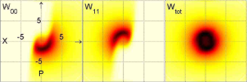
Refer to caption
Figure 5.2: Shuttling at zero electric field. The three Wigner distributions for the empty, charged, and sum states are represented in the usual adimensional phase space (X,P)𝑋𝑃(X,P) (see Fig. 5.1). The parameter values are λ=x0𝜆subscript𝑥0\lambda=x_{0}, T=0𝑇0T=0, d=0𝑑0d=0, Γ=0.05ωΓ0.05𝜔\Gamma=0.05\omega, γ=0𝛾0\gamma=0.

The amplitude of the shuttling oscillations of the quantum dot is also dependent on the tunneling length and bare injection rate. In particular it grows with the tunneling length λ𝜆\lambda and with the inverse of the bare injection rate.
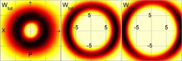
Refer to caption
Figure 5.3: Transition from “quantum” to “classical” shuttling. The figure shows the total Wigner function for three different sets of parameters. We keep constant damping (γ=0.02ω𝛾0.02𝜔\gamma=0.02\omega) temperature (T=0𝑇0T=0) and electric field (d=0.5x0𝑑0.5subscript𝑥0d=0.5x_{0}) and change the injection rate and tunneling length. From left to right respectively: (Γ=0.05ω,λ=x0)formulae-sequenceΓ0.05𝜔𝜆subscript𝑥0(\Gamma=0.05\omega,\,\lambda=x_{0}), (Γ=0.05ω,λ=2x0)formulae-sequenceΓ0.05𝜔𝜆2subscript𝑥0(\Gamma=0.05\omega,\,\lambda=2x_{0}), (Γ=0.01ω,λ=2x0)formulae-sequenceΓ0.01𝜔𝜆2subscript𝑥0(\Gamma=0.01\omega,\,\lambda=2x_{0}).

This behavior can be understood as a self-consistent compensation to accomplish the non-adiabatic condition that the effective injection rate Γ¯¯Γ\bar{\Gamma} must be comparable in the shuttling regime with the oscillator frequency ω/2π𝜔2𝜋\omega/2\pi. The larger the amplitude of the oscillation the more classical is the behavior of the harmonic oscillator. This concept can be understood also from a geometric point of view: the ring gets closer and closer to a circle since the width, given by the amount of thermal and shot noise remains constant (or decreases as we will see in the coexistence regime semianalytics) while the diameter increases. Another natural parameter that reveals this quantum to classical transition is the ratio between Planck-constant-over-2-pi\hbar and the area enclosed by the ring. This tends to zero in the classical limit (Fig. 5.3).

5.1.3 Different electronic processes in the TDQS

The Wigner distribution analysis of the TDQS is performed in analogy with the SDQS on the states corresponding to the empty and charged central dot. Namely we consider:

WUUstat(q,p)=12π+𝑑ξqξ2|σ00stat+σLLstat+σRRstat|q+ξ2exp(ipξ)WCCstat(q,p)=12π+𝑑ξqξ2|σCCstat|q+ξ2exp(ipξ)superscriptsubscript𝑊𝑈𝑈stat𝑞𝑝12𝜋Planck-constant-over-2-pisuperscriptsubscriptdifferential-d𝜉quantum-operator-product𝑞𝜉2superscriptsubscript𝜎00statsuperscriptsubscript𝜎𝐿𝐿statsuperscriptsubscript𝜎𝑅𝑅stat𝑞𝜉2𝑖𝑝𝜉Planck-constant-over-2-pisuperscriptsubscript𝑊𝐶𝐶stat𝑞𝑝12𝜋Planck-constant-over-2-pisuperscriptsubscriptdifferential-d𝜉quantum-operator-product𝑞𝜉2superscriptsubscript𝜎𝐶𝐶stat𝑞𝜉2𝑖𝑝𝜉Planck-constant-over-2-pi\begin{split}W_{UU}^{\rm stat}(q,p)&=\frac{1}{2\pi\hbar}\int_{-\infty}^{+\infty}\!\!\!d\xi\left\langle q-\frac{\xi}{2}\right|\sigma_{00}^{\rm stat}+\sigma_{LL}^{\rm stat}+\sigma_{RR}^{\rm stat}\left|q+\frac{\xi}{2}\right\rangle\exp\left(\frac{ip\xi}{\hbar}\right)\\ W_{CC}^{\rm stat}(q,p)&=\frac{1}{2\pi\hbar}\int_{-\infty}^{+\infty}\!\!\!d\xi\left\langle q-\frac{\xi}{2}\right|\sigma_{CC}^{\rm stat}\left|q+\frac{\xi}{2}\right\rangle\exp\left(\frac{ip\xi}{\hbar}\right)\end{split} (5.3)

As suggested by the work of Armour and MacKinnon [7] we consider as control parameter the difference between the gate voltages on the left and right dot (the so-called device bias ΔVΔ𝑉\Delta V). It was found in [7] that the triple dot system exhibits different regimes of transport at different device biases. The current peaks at ΔVnωΔ𝑉𝑛Planck-constant-over-2-pi𝜔\Delta V\approx n\hbar\omega were identified as effects of electromechanical resonances within the device. Yet, the different peaks may correspond to different physical mechanisms – while the peak around ΔVωΔ𝑉Planck-constant-over-2-pi𝜔\Delta V\approx\hbar\omega is mainly due to the incoherent oscillator-assisted tunneling the peak at ΔV2ωΔ𝑉2Planck-constant-over-2-pi𝜔\Delta V\approx 2\hbar\omega reveals a clear shuttling component. This finding by Armour and MacKinnon based on indirect evidence of parametric dependencies of the current curves (e.g. the dependence of the current curve on the tunneling length λ𝜆\lambda) is confirmed by the direct inspection of the phase space distribution (Fig. 5.4). The half-moon-like shape characteristic for the shuttling transport is only present around ΔV2ωΔ𝑉2𝜔\Delta V\approx 2\omega while all other plots show just the fuzzy spot indicative of incoherent tunneling. However, our direct criterion for detecting the shuttling regime reveals a close similarity between the resonances. For increasing injection rate we can see that the shuttling regime gradually sets in also in the vicinity of the first resonance peak. This reveals the cross over character of the onset of the shuttling instability found also for the SDQS.
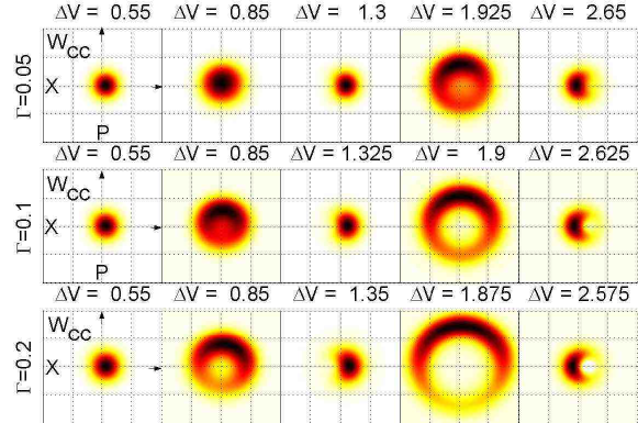
Refer to caption
Figure 5.4: Wigner distributions for the central dot in the charged state. The half-moon shuttling signature, always present at the second resonance (ΔV2ωΔ𝑉2Planck-constant-over-2-pi𝜔\Delta V\approx 2\hbar\omega) progressively emerges also in the first resonance (ΔVωΔ𝑉Planck-constant-over-2-pi𝜔\Delta V\approx\hbar\omega). The other parameters are V0=0.757ω,λ=5Δxz,x0=7.071Δxz,γ=0.0125ωformulae-sequencesubscript𝑉00.757Planck-constant-over-2-pi𝜔formulae-sequence𝜆5Δsubscript𝑥𝑧formulae-sequencesubscript𝑥07.071Δsubscript𝑥𝑧𝛾0.0125𝜔V_{0}=0.757\hbar\omega,\,\lambda=5\Delta x_{z},\,x_{0}=7.071\Delta x_{z},\,\gamma=0.0125\omega.

As can be seen in more detail in the work by C. Flindt et al. [33] and in the Master thesis by C. Flindt [12] the TDQS exhibits at higher device biases another transport mechanism that competes with the shuttling transport. For ΔV3ω,4ωΔ𝑉3𝜔4𝜔\Delta V\approx 3\omega,4\omega inelastic co-tunneling takes place and a clear signature of this phenomenon can be seen in the vanishing of the charged central dot Wigner function (see Fig. 5 in [33]).

5.2 Current

The Wigner distribution functions are a very clean theoretical tool to investigate the dynamical properties of shuttle devices, but unfortunately it seems very difficult (if not impossible) to access experimentally these functions. For this reason, with in mind the distribution function description, we investigate the electronic transport properties in the shuttle devices (more realistically measurable) starting with the stationary current.

5.2.1 Calculation of the stationary current

We already encountered in section 3.3.5 the definition of right and left lead currents:

IR(t)=N˙R(t)IL(t)=N˙L(t)subscript𝐼𝑅𝑡subscript˙𝑁𝑅𝑡subscript𝐼𝐿𝑡subscript˙𝑁𝐿𝑡\begin{split}I_{R}(t)&=\dot{N}_{R}(t)\\ I_{L}(t)&=\dot{N}_{L}(t)\end{split} (5.4)

where NR(t)subscript𝑁𝑅𝑡N_{R}(t) (NL(t)subscript𝑁𝐿𝑡N_{L}(t)) are the total number of electrons (holes) collected in the right (left) lead at time t𝑡t. We have also related these functions to the elements of the n𝑛n(hh)-resolved density matrix and corresponding GME (Eq. (3.54) and (3.56)). Since we are interested exclusively in the stationary current333The stationary current is equal on both leads due to charge conservation. we analyze now in detail only the electron current in the right lead in presence of a shuttle device (SDQS or TDQS). The total number of electrons collected in the right lead NR(t)subscript𝑁𝑅𝑡N_{R}(t) can be written as:

NR(t)=n=0nPn(t)subscript𝑁𝑅𝑡superscriptsubscript𝑛0𝑛subscript𝑃𝑛𝑡N_{R}(t)=\sum_{n=0}^{\infty}nP_{n}(t) (5.5)

where Pn(t)subscript𝑃𝑛𝑡P_{n}(t) is the probability for n𝑛n electrons to be collected into the right lead at time t𝑡t. We express the probability Pn(t)subscript𝑃𝑛𝑡P_{n}(t) as the trace of the n𝑛n-resolved reduced density matrix over the system degrees of freedom:

Pn(t)=Trsys{σ(n)(t)}=Trosc{iσii(n)(t)}subscript𝑃𝑛𝑡subscriptTrsyssuperscript𝜎𝑛𝑡subscriptTroscsubscript𝑖superscriptsubscript𝜎𝑖𝑖𝑛𝑡P_{n}(t)={\rm Tr}_{\rm sys}\left\{\sigma^{(n)}(t)\right\}={\rm Tr}_{\rm osc}\left\{\textstyle{\sum_{i}}\sigma_{ii}^{(n)}(t)\right\} (5.6)

where i𝑖i is the electrical state of the device: and in the SDQS i=0,1𝑖01i=0,1 while in the TDQS i=0,L,C,R𝑖0𝐿𝐶𝑅i=0,L,C,R. The n𝑛n-resolved GME (n𝑛n-GME) comes now into play and the current is expressed as a function of σii(n)(t)superscriptsubscript𝜎𝑖𝑖𝑛𝑡\sigma_{ii}^{(n)}(t):

IR(t)=n=0inTrosc{σ˙ii(n)(t)}=n=0niTrosc{coh[σ(n)(t)]ii+driv[σ(t)]ii(n)+damp[σii(n)(t)]}subscript𝐼𝑅𝑡superscriptsubscript𝑛0subscript𝑖𝑛subscriptTroscsuperscriptsubscript˙𝜎𝑖𝑖𝑛𝑡superscriptsubscript𝑛0𝑛subscript𝑖subscriptTroscsubscriptcohsubscriptdelimited-[]superscript𝜎𝑛𝑡𝑖𝑖subscriptdrivsubscriptsuperscriptdelimited-[]𝜎𝑡𝑛𝑖𝑖subscriptdampdelimited-[]subscriptsuperscript𝜎𝑛𝑖𝑖𝑡\begin{split}I_{R}(t)&=\sum_{n=0}^{\infty}\sum_{i}n{\rm Tr}_{\rm osc}\left\{\dot{\sigma}_{ii}^{(n)}(t)\right\}\\ &=\sum_{n=0}^{\infty}n\sum_{i}{\rm Tr}_{\rm osc}\left\{\mathcal{L}_{\rm coh}\big{[}\sigma^{(n)}(t)\big{]}_{ii}+\mathcal{L}_{\rm driv}\big{[}\sigma(t)\big{]}^{(n)}_{ii}+\mathcal{L}_{\rm damp}\big{[}\sigma^{(n)}_{ii}(t)\big{]}\right\}\end{split} (5.7)

where we have implicitly specified with the position of the square parentheses the different components of the density matrix addressed by the different Liouvilleans444The damping Liouvillean acts only in the Hilbert space of the harmonic oscillator and does not mix different electronic states or states with different number of particle in the collector. The coherent Liouvillean is sensitive to the charge state of the system and does not care about the particular bath state, while the driving term is mixing electronic states and bath states with different number of particles since it describes the electron tunneling between system and baths. All of them are local in time (Markov approximation)..

We calculate first the SDQS right (particle) current. The coherent and damping part of the Liouvillean have a commutator structure (see Eq. (3.116)) and vanish under trace. We are left with the contribution given by the driving Liouvillean:

IR(t)=Trosc{ΓRe2x/λn=0n[σ11(n1)(t)σ11(n)(t)]}subscript𝐼𝑅𝑡subscriptTroscsubscriptΓ𝑅superscript𝑒2𝑥𝜆superscriptsubscript𝑛0𝑛delimited-[]superscriptsubscript𝜎11𝑛1𝑡superscriptsubscript𝜎11𝑛𝑡I_{R}(t)={\rm Tr}_{\rm osc}\left\{\Gamma_{R}e^{2x/\lambda}\sum_{n=0}^{\infty}n\left[\sigma_{11}^{(n-1)}(t)-\sigma_{11}^{(n)}(t)\right]\right\} (5.8)

where we have used the cyclic property of the trace to evaluate the sum over the two electrical components. The particular ordering of the position dependent injection and ejection operators ΓL,R(x)subscriptΓ𝐿𝑅𝑥\Gamma_{L,R}(x) is irrelevant under trace and the sum over the number of electron in the resevoir is formally identical to the one obtained for the static single dot (see Eq. (3.54)). We evaluate it and obtain:

IR(t)=Trosc{ΓRe2x/λσ11(t)}subscript𝐼𝑅𝑡subscriptTroscsubscriptΓ𝑅superscript𝑒2𝑥𝜆subscript𝜎11𝑡I_{R}(t)={\rm Tr}_{\rm osc}\left\{\Gamma_{R}e^{2x/\lambda}\sigma_{11}(t)\right\} (5.9)

With completely analogous arguments one derives the expression for the left current:

IL(t)=Trosc{ΓLe2x/λσ00(t)}subscript𝐼𝐿𝑡subscriptTroscsubscriptΓ𝐿superscript𝑒2𝑥𝜆subscript𝜎00𝑡I_{L}(t)={\rm Tr}_{\rm osc}\left\{\Gamma_{L}e^{-2x/\lambda}\sigma_{00}(t)\right\} (5.10)

The stationary current is obtained by substituting in (5.9) or (5.10) the stationary solution σstatsuperscript𝜎stat\sigma^{\rm stat} of the GME. It is interesting that the stationary particle current is written as the average injection (ejection) rate:

Istat=Trosc{ΓRe2x/λσ11stat}=Trsys{ΓR(x)|11|σstat}=Γ¯RTrosc{ΓLe2x/λσ00stat}=Trsys{ΓL(x)|00|σstat}=Γ¯L=Γ¯superscript𝐼statsubscriptTroscsubscriptΓ𝑅superscript𝑒2𝑥𝜆subscriptsuperscript𝜎stat11subscriptTrsyssubscriptΓ𝑅𝑥ket1bra1superscript𝜎statsubscript¯Γ𝑅missing-subexpressionmissing-subexpressionsubscriptTroscsubscriptΓ𝐿superscript𝑒2𝑥𝜆subscriptsuperscript𝜎stat00subscriptTrsyssubscriptΓ𝐿𝑥ket0bra0superscript𝜎statsubscript¯Γ𝐿¯ΓI^{\rm stat}=\begin{array}[]{c}\nearrow\\ \searrow\end{array}\begin{array}[]{c}{\rm Tr}_{\rm osc}\left\{\Gamma_{R}e^{2x/\lambda}\sigma^{\rm stat}_{11}\right\}={\rm Tr}_{\rm sys}\left\{\Gamma_{R}(x)|1\rangle\!\langle 1|\sigma^{\rm stat}\right\}=\bar{\Gamma}_{R}\\ \\ \\ {\rm Tr}_{\rm osc}\left\{\Gamma_{L}e^{-2x/\lambda}\sigma^{\rm stat}_{00}\right\}={\rm Tr}_{\rm sys}\left\{\Gamma_{L}(x)|0\rangle\!\langle 0|\sigma^{\rm stat}\right\}=\bar{\Gamma}_{L}\end{array}\begin{array}[]{c}\searrow\\ \nearrow\end{array}=\bar{\Gamma} (5.11)

where we have introduced the projectors |11|c1c1ket1bra1superscriptsubscript𝑐1superscriptsubscript𝑐1absent|1\rangle\!\langle 1|\equiv c_{1}^{{\dagger}}c_{1}^{\phantom{\dagger}} and |00|1c1c1ket0bra01superscriptsubscript𝑐1superscriptsubscript𝑐1absent|0\rangle\!\langle 0|\equiv 1-c_{1}^{{\dagger}}c_{1}^{\phantom{\dagger}} on the electronic Hilbert space and we calculate the average injection and ejection rates taking into account Coulomb blockade and the single level structure. Namely the injection (ejection) rate average is calculated only on system states with empty (charged) dot. A special remark concerns correlations: the shuttling regime is characterized by strong electromechanical correlations and they should be recorded in the current since in general:

Istat=Trsys{ΓL(x)|00|σstat}Trsys{ΓL(x)σstat}Trsys{|00|σstat}superscript𝐼statsubscriptTrsyssubscriptΓ𝐿𝑥ket0bra0superscript𝜎statsubscriptTrsyssubscriptΓ𝐿𝑥superscript𝜎statsubscriptTrsysket0bra0superscript𝜎statI^{\rm stat}={\rm Tr}_{\rm sys}\{\Gamma_{L}(x)|0\rangle\!\langle 0|\sigma^{\rm stat}\}\neq{\rm Tr}_{\rm sys}\{\Gamma_{L}(x)\sigma^{\rm stat}\}{\rm Tr}_{\rm sys}\{|0\rangle\!\langle 0|\sigma^{\rm stat}\} (5.12)

5.2.2 Current characteristics of the SDQS

We study the current as a function of the mechanical damping. The results for different values of the bare injection (ejection) rate and of the tunneling length are presented in Fig. 5.5. At low damping the current saturates, independently from the value of the other parameters, at the “magic” value I0.16ω𝐼0.16𝜔I\approx 0.16\omega (numerical approximation of the frequency of the harmonic oscillator ω/2π𝜔2𝜋\omega/2\pi). Increasing the damping the stationary current drops, more or less rapidly, to a plateau, dependent this time on both the bare tunneling rate and length. Further increase of the damping does not change the scenario. The transition between the plateau and the saturation point is faster the more “classical” the other parameters are (i.e. small injection rate and large tunneling length555See previous section for the meaning of the term “classical” associated to a parameter configuration.).
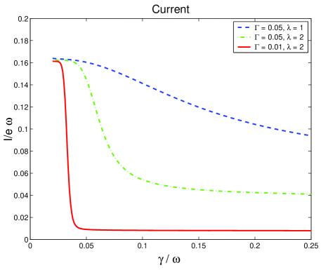
Refer to caption
Figure 5.5: Particle stationary current of the SDQS plotted as a function of the damping rate. The bare electronic rate (Γ)Γ(\Gamma) is given in units of the oscillator frequency. The tunneling length is given in units of x0=/mωsubscript𝑥0Planck-constant-over-2-pi𝑚𝜔x_{0}=\sqrt{\hbar/m\omega}. The current and the damping rate are expressed in adimensional units also by rescaling with the oscillator frequency ω𝜔\omega. The saturation of the current to the limit of one electron per cycle characteristic of the shuttling regime at low damping is visible. The transition to the the high damping limit (oscillator in ground state) gets sharper the more classical is the dynamics as is indicated also by the parameters (see text for explanation).

If we compare the current results with the Wigner function distribution we can recognize a correspondence between the shuttling charge-position (momentum) correlation and the saturation point, as well as a progressive disappearing of the ring structure in correspondence with the current transition. The high damping plateau in the current sets in when the mechanical oscillator lays into its ground state and the Wigner distribution function is reduced to a fuzzy spot close to the origin of the phase space (Fig. 5.6).
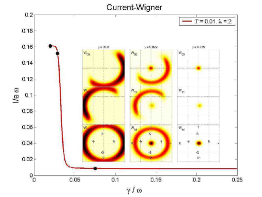
Refer to caption
Figure 5.6: Most “classical” current-damping curve. The Wigner function distributions in the insets correspond to the three dots indicated on the curve and show how the transition looks like in the phase space.

5.2.3 Electromechanical resonances of the TDQS

The calculation of the TDQS stationary current follows the same argument line we adopted for the SDQS. Also the analytic expression shares essentially the same structure, the only difference being the projector that appears in the right lead current and the tunneling rate that in this case is not position dependent. The electrons tunnel to the resevoir only from the right dot and the current reads:

IRstat=ΓRTrosc{σRRstat}=ΓRTrsys{|RR|σstat}=Γ¯Rsuperscriptsubscript𝐼𝑅statsubscriptΓ𝑅subscriptTroscsubscriptsuperscript𝜎stat𝑅𝑅subscriptΓ𝑅subscriptTrsysket𝑅bra𝑅superscript𝜎statsubscript¯Γ𝑅I_{R}^{\rm stat}=\Gamma_{R}{\rm Tr}_{\rm osc}\left\{\sigma^{\rm stat}_{RR}\right\}=\Gamma_{R}{\rm Tr}_{\rm sys}\left\{|R\rangle\!\langle R|\sigma^{\rm stat}\right\}=\bar{\Gamma}_{R} (5.13)

Since there are not position operators in the left or right lead current one could argue that the stationary current of the TDQS do not record signs of charge-position correlation. The solution to this problem comes from the structure of the device. Instead of looking at the system-lead tunneling current one can concentrate on the tunneling current within the device: in the stationary limit charge conservation ensures they are equal. For example the left-center current reads in the stationary limit:

ILCstat=Trosc{itL(x)(σCLstatσLCstat)}superscriptsubscript𝐼𝐿𝐶statsubscriptTrosc𝑖subscript𝑡𝐿𝑥subscriptsuperscript𝜎stat𝐶𝐿subscriptsuperscript𝜎stat𝐿𝐶I_{LC}^{\rm stat}={\rm Tr}_{\rm osc}\{it_{L}(x)(\sigma^{\rm stat}_{CL}-\sigma^{\rm stat}_{LC})\} (5.14)

as can be derived tracing the second equation of (3.131).

A detailed analysis of the current in the TDQS with the device bias666We recall that the device bias is defined as the difference between the gate voltages of the left and right dot and is represented in the model (Eq. (2.9)) as the mismatch between the left and right dot energy levels (ΔVΔ𝑉\Delta V). as control parameter can be found in the work by Armour and MacKinnon [7]. Extension and analysis of the same model in other parameter regimes are given in [11] and extensively in [12] and [33]. Qualitatively we can describe the current-device bias characteristics as series of peaks (electromechanical resonancies) at ΔVnωΔ𝑉𝑛Planck-constant-over-2-pi𝜔\Delta V\approx n\hbar\omega. It is difficult to establish only from the analysis of the current the nature of these peaks. Armour and MacKinnon have an interpretation of the different mechanisms underlying these resonances based on the analysis of the spectrum of the decoupled three dot device + harmonic oscillator. This method can visualize very well the basic mechanisms of elastic or inelastic phonon assisted tunneling. Other information can be gained from the behaviour of the current at different resonances as a function of the tunneling length or mechanical damping. We acknowledge the validity of this analysis but we also think that an independent source of information (such as the phase space or the current-noise) is needed to discriminate directly between different operating regimes. In Fig. 5.7 we report a set of current curves in which one can recognize the first three electromechanical resonances.
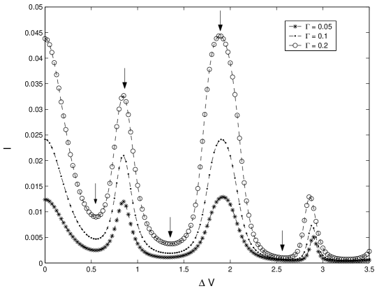
Refer to caption
Figure 5.7: Current as function of device bias in TDQS. Different curves correspond to different injection rates ΓΓ\Gamma. The particle current and the injection rate ΓΓ\Gamma are scaled with the mechanical frequency ω𝜔\omega. The first three electromechanical resonances are visible. The arrows indicate points of minimum or maximum current and the corresponding Wigner distributions are reported in Fig. 5.4. The other parameters are V0=0.757ω,λ=5Δxz,x0=7.071Δxz,γ=0.0125ωformulae-sequencesubscript𝑉00.757Planck-constant-over-2-pi𝜔formulae-sequence𝜆5Δsubscript𝑥𝑧formulae-sequencesubscript𝑥07.071Δsubscript𝑥𝑧𝛾0.0125𝜔V_{0}=0.757\hbar\omega,\,\lambda=5\Delta x_{z},\,x_{0}=7.071\Delta x_{z},\,\gamma=0.0125\omega.

The temperature influences the device characteristics in different ways since different competing transport mechanisms (phonon assisted-tunneling, co-tunneling, shuttling) depend on temperature in very different ways. A generic feature can though be recognized: at finite temperature electromechanical resonances are found also at negative device biases (see for example Fig. 2 in [33]) when electrons can tunnel through the device only by gaining energy from the oscillator. This observation suggests the idea of an active phonon cooling device777This idea was suggested by prof. K. Mølmer during private communications. useful to prepare for example a macroscopic harmonic oscillator close to its quantum ground state more efficiently than by coupling it to a “very cold” thermal resevoir.

5.3 Current noise

An unequivocal experimental observation of the shuttling transition has not yet been achieved. The IV-curve measured in recent experiments on a vibrating C60subscriptC60{\rm C_{60}} can be interpreted in terms of shuttling [19], but also alternative explanations have been promoted [20, 21, 36]. It is therefore natural to look for more refined experimental tools than just the average current through the device. An obvious candidate is the current noise spectrum [37, 38]. The measurement of the noise spectrum or even higher moments (full counting statistics) reveals more information about the transport through the device than just the mean current. The theoretical studies of the noise have attracted much attention recently in NEMS in general [39, 40, 41] as well as for the shuttling set up [5, 42, 14] in the (semi)classical limit. The quantum mechanical theory for shot noise in NEMS that we treat here is also exposed in [23] and in a more general form in [33] and is mainly due to T. Novotný in collaboration with the author and C. Flindt.

5.3.1 The MacDonald formula

Let us consider the (particle) current flowing from the dot to the right lead of the SDQS. This is defined (in the Heisenberg picture) as the time derivative of the number operator of the right lead:

I^R(t)=N^˙R(t)=i[H^(t),N^R(t)]=iT^r(x^)k(c^rkc^1+c^1c^rk)subscript^𝐼𝑅𝑡subscript˙^𝑁𝑅𝑡𝑖Planck-constant-over-2-pi^𝐻𝑡subscript^𝑁𝑅𝑡𝑖Planck-constant-over-2-pisubscript^𝑇𝑟^𝑥subscript𝑘subscriptsuperscript^𝑐subscript𝑟𝑘subscriptsuperscript^𝑐absent1subscriptsuperscript^𝑐1subscriptsuperscript^𝑐absentsubscript𝑟𝑘\begin{split}\hat{I}_{R}(t)&=\dot{\hat{N}}_{R}(t)=-\frac{i}{\hbar}[\hat{H}(t),\hat{N}_{R}(t)]\\ &=-\frac{i}{\hbar}\hat{T}_{r}(\hat{x})\sum_{k}\left(\hat{c}^{{\dagger}}_{r_{k}}\hat{c}^{\phantom{\dagger}}_{1}+\hat{c}^{{\dagger}}_{1}\hat{c}^{\phantom{\dagger}}_{r_{k}}\right)\end{split} (5.15)

where

NR=kcrkcrk,subscript𝑁𝑅subscript𝑘subscriptsuperscript𝑐subscript𝑟𝑘subscriptsuperscript𝑐absentsubscript𝑟𝑘N_{R}=\sum_{k}c^{{\dagger}}_{r_{k}}c^{\phantom{\dagger}}_{r_{k}}, (5.16)

the symbol ^^\hat{\bullet} indicates the Heisenberg picture and H𝐻H is the Hamiltonian presented in equation (2.1,2.2). The current-current correlation function of right currents reads:

CIR,IR(t,t)=12{I^R(t),I^R(t)}I^R(t)I^R(t)subscript𝐶subscript𝐼𝑅subscript𝐼𝑅𝑡superscript𝑡12delimited-⟨⟩subscript^𝐼𝑅𝑡subscript^𝐼𝑅superscript𝑡delimited-⟨⟩subscript^𝐼𝑅𝑡delimited-⟨⟩subscript^𝐼𝑅superscript𝑡C_{I_{R},I_{R}}(t,t^{\prime})=\frac{1}{2}\langle\{\hat{I}_{R}(t),\hat{I}_{R}(t^{\prime})\}\rangle-\langle\hat{I}_{R}(t)\rangle\langle\hat{I}_{R}(t^{\prime})\rangle (5.17)

and the brackets \langle\phantom{a}\rangle indicate the quantum mechanical average888Since we work in Heisenberg picture the quantum average is given by the expectation value on the initial state – i.e. at the time when the Schrödinger and Heisenberg pictures coincide.. The noise spectrum is defined as the Fourier transform of the correlation function999Some authors define this Fourier with an extra factor of 2 at the numerator. A balancing factor of 2 at the denominator is then inserted in the definition of the Fano factor.:

SRR(ω)=limt+𝑑τCIR,IR(t+τ,t)eiωτsubscript𝑆𝑅𝑅𝜔subscript𝑡superscriptsubscriptdifferential-d𝜏subscript𝐶subscript𝐼𝑅subscript𝐼𝑅𝑡𝜏𝑡superscript𝑒𝑖𝜔𝜏S_{RR}(\omega)=\lim_{t\to\infty}\int_{-\infty}^{+\infty}d\tau\,C_{I_{R},I_{R}}(t+\tau,t)\,e^{i\omega\tau} (5.18)

It is possible to demonstrate (see for example [33]) that the zero frequency component of the current noise is independent from the particular junction considered. We will for this reason speak in general of current noise S(ω=0)𝑆𝜔0S(\omega=0) even if the specific realization of the calculation refers to the right junction current. Multitime averages (e.g. (5.17)) can be evaluated in general using the Quantum Regression Theorem [27]. Necessary condition is though the fact that the operators averaged must belong to the system. This condition is obviously violated by the operator I^R(t)subscript^𝐼𝑅𝑡\hat{I}_{R}(t) defined in equation (5.15) that contains system and bath operators. An alternative way of calculating the current noise relates it to the probability Pn(t)subscript𝑃𝑛𝑡P_{n}(t) that n𝑛n electrons have tunnelled through the device by the time t𝑡t.

We now present this alternative formulation101010One of the main reasons for the extensive derivation of the n𝑛n-GME that we gave in chapter 3 is this formulation of the SDQS current noise.. Let us take the definition of noise spectrum (5.18) in the zero frequency limit and consider the symmetry relation

limtCIR,IR(t+τ,t)=limtCIR,IR(tτ,t)subscript𝑡subscript𝐶subscript𝐼𝑅subscript𝐼𝑅𝑡𝜏𝑡subscript𝑡subscript𝐶subscript𝐼𝑅subscript𝐼𝑅𝑡𝜏𝑡\lim_{t\to\infty}C_{I_{R},I_{R}}(t+\tau,t)=\lim_{t\to\infty}C_{I_{R},I_{R}}(t-\tau,t) (5.19)

and the definition of the current operator (5.15). We can rewrite the noise in the form:

S(0)=limt[{limτ[N^R(τ)N^R(0)],ddt[N^R(t)N^R(0)]}2limτ[N^R(τ)N^R(0)]ddt[N^R(t)N^R(0)]]𝑆0subscript𝑡delimited-[]delimited-⟨⟩subscript𝜏delimited-[]subscript^𝑁𝑅𝜏subscript^𝑁𝑅0𝑑𝑑𝑡delimited-[]subscript^𝑁𝑅𝑡subscript^𝑁𝑅02delimited-⟨⟩subscript𝜏delimited-[]subscript^𝑁𝑅𝜏subscript^𝑁𝑅0delimited-⟨⟩𝑑𝑑𝑡delimited-[]subscript^𝑁𝑅𝑡subscript^𝑁𝑅0\begin{split}S(0)=&\lim_{t\to\infty}\Big{[}\langle\big{\{}\lim_{\tau\to\infty}[\hat{N}_{R}(\tau)-\hat{N}_{R}(0)],\frac{d}{dt}[\hat{N}_{R}(t)-\hat{N}_{R}(0)]\big{\}}\rangle\\ &-2\langle\lim_{\tau\to\infty}[\hat{N}_{R}(\tau)-\hat{N}_{R}(0)]\rangle\langle\frac{d}{dt}[\hat{N}_{R}(t)-\hat{N}_{R}(0)]\rangle\Big{]}\end{split} (5.20)

where we have also used the property:

limτlimtN^R(t+τ)N^R(t)limτN^R(τ)N^R(0)similar-tosubscript𝜏subscript𝑡subscript^𝑁𝑅𝑡𝜏subscript^𝑁𝑅𝑡subscript𝜏subscript^𝑁𝑅𝜏subscript^𝑁𝑅0\lim_{\tau\to\infty}\lim_{t\to\infty}\hat{N}_{R}(t+\tau)-\hat{N}_{R}(t)\sim\lim_{\tau\to\infty}\hat{N}_{R}(\tau)-\hat{N}_{R}(0) (5.21)

where with the symbol similar-to\sim we mean that they have the same asymptotic behaviour. This property is a direct consequence of a large times stationary current.

Finally, by inserting the definition of transferred charge operator Q^R(t)N^R(t)N^R(0)subscript^𝑄𝑅𝑡subscript^𝑁𝑅𝑡subscript^𝑁𝑅0\hat{Q}_{R}(t)\equiv\hat{N}_{R}(t)-\hat{N}_{R}(0) into (5.20), we obtain:

S(0)=limtddt[Q^R2(t)Q^R(t)2]𝑆0subscript𝑡𝑑𝑑𝑡delimited-[]delimited-⟨⟩superscriptsubscript^𝑄𝑅2𝑡superscriptdelimited-⟨⟩subscript^𝑄𝑅𝑡2S(0)=\lim_{t\to\infty}\frac{d}{dt}\Big{[}\langle\hat{Q}_{R}^{2}(t)\rangle-\langle\hat{Q}_{R}(t)\rangle^{2}\Big{]} (5.22)

In the basis in which the transferred charge operator is diagonal we can express the quantum expectation values111111In what follows we assume the equivalence between the Heisenberg and Schrödinger picture and evaluate the averages in the latter representation. of Q𝑄Q and Q2superscript𝑄2Q^{2} using the corresponding diagonal density matrix121212Note that in this basis the density matrix is diagonal since the state of the right bath is a statistical mixture of states with different particle numbers. Pn(t)subscript𝑃𝑛𝑡P_{n}(t) and we obtain:

S(0)=limt+ddt[n=0n2Pn(t)(n=0nPn(t))2]𝑆0subscript𝑡𝑑𝑑𝑡delimited-[]superscriptsubscript𝑛0superscript𝑛2subscript𝑃𝑛𝑡superscriptsuperscriptsubscript𝑛0𝑛subscript𝑃𝑛𝑡2S(0)=\lim_{t\to+\infty}\frac{d}{dt}\Big{[}\sum_{n=0}^{\infty}n^{2}P_{n}(t)-\big{(}\sum_{n=0}^{\infty}nP_{n}(t)\big{)}^{2}\Big{]} (5.23)

known as the MacDonald formula [43]. This formula represents the starting point for the calculation of the noise in the shuttle devices. We analyze in detail the SDQS case. The TDQS case is the main subject of a detailed article [33] and of the Master thesis of C. Flindt [12] and we direct the interested reader to that literature.

5.3.2 Current noise in the SDQS

The shot noise is completely determined by the evaluation of large times asymptotics of the functions:

A(t)=n=0nPn(t),B(t)=n=0nP˙n(t),C(t)=n=0n2P˙n(t)formulae-sequence𝐴𝑡superscriptsubscript𝑛0𝑛subscript𝑃𝑛𝑡formulae-sequence𝐵𝑡superscriptsubscript𝑛0𝑛subscript˙𝑃𝑛𝑡𝐶𝑡superscriptsubscript𝑛0superscript𝑛2subscript˙𝑃𝑛𝑡A(t)=\sum_{n=0}^{\infty}nP_{n}(t),\quad B(t)=\sum_{n=0}^{\infty}n\dot{P}_{n}(t),\quad C(t)=\sum_{n=0}^{\infty}n^{2}\dot{P}_{n}(t) (5.24)

that appear in the MacDonald formula if one explicitly calculates the time derivative. We recognize in A(t)𝐴𝑡A(t) the average number of electrons NR(t)subscript𝑁𝑅𝑡N_{R}(t) tunnelled to the right lead by the time t𝑡t and in B(t)𝐵𝑡B(t) the right lead current IR(t)subscript𝐼𝑅𝑡I_{R}(t). From the previous section we know the asymptotic behaviour of the the current at large times:

limtIR(t)=Trosc{ΓRe2x/λσ11stat}subscript𝑡subscript𝐼𝑅𝑡subscriptTroscsubscriptΓ𝑅superscript𝑒2𝑥𝜆subscriptsuperscript𝜎stat11\lim_{t\to\infty}I_{R}(t)={\rm Tr}_{\rm osc}\left\{\Gamma_{R}e^{2x/\lambda}\sigma^{\rm stat}_{11}\right\} (5.25)

Using the n𝑛n-GME we can express also the C𝐶C function in terms of the reduced density matrices σ11(n)superscriptsubscript𝜎11𝑛\sigma_{11}^{(n)}

C(t)=n=0n2P˙n(t)=n=0n2ΓRTrosc[e2x/λ(σ11(n1)σ11(n))]=n=02nTrosc[ΓRe2x/λσ11(n)]+ΓRTrosc[e2x/λσ11]𝐶𝑡superscriptsubscript𝑛0superscript𝑛2subscript˙𝑃𝑛𝑡superscriptsubscript𝑛0superscript𝑛2subscriptΓ𝑅subscriptTroscdelimited-[]superscript𝑒2𝑥𝜆superscriptsubscript𝜎11𝑛1superscriptsubscript𝜎11𝑛superscriptsubscript𝑛02𝑛subscriptTroscdelimited-[]subscriptΓ𝑅superscript𝑒2𝑥𝜆superscriptsubscript𝜎11𝑛subscriptΓ𝑅subscriptTroscdelimited-[]superscript𝑒2𝑥𝜆subscript𝜎11\begin{split}C(t)=\sum_{n=0}^{\infty}n^{2}\dot{P}_{n}(t)&=\sum_{n=0}^{\infty}n^{2}\Gamma_{R}{\rm Tr}_{\rm osc}\big{[}e^{2x/\lambda}(\sigma_{11}^{(n-1)}-\sigma_{11}^{(n)})\big{]}\\ &=\sum_{n=0}^{\infty}2n{\rm Tr}_{\rm osc}\big{[}\Gamma_{R}e^{2x/\lambda}\sigma_{11}^{(n)}\big{]}+\Gamma_{R}{\rm Tr}_{\rm osc}\big{[}e^{2x/\lambda}\sigma_{11}\big{]}\end{split} (5.26)

where we have used the boundary condition σ11(1)0superscriptsubscript𝜎1110\sigma_{11}^{(-1)}\equiv 0 due to the high bias limit that does not allow electrons to enter from the right lead. It is convenient for the calculation of the t𝑡t\to\infty limit in (5.23) to introduce the generating functions131313These are in fact an operator-valued generalization of the generating function concept.:

Fii(t;z)=n=0σii(n)(t)znsubscript𝐹𝑖𝑖𝑡𝑧superscriptsubscript𝑛0superscriptsubscript𝜎𝑖𝑖𝑛𝑡superscript𝑧𝑛F_{ii}(t;z)=\sum_{n=0}^{\infty}\sigma_{ii}^{(n)}(t)z^{n} (5.27)

with the properties:

Fii(t;1)=σii(t)zFii(t;z)|z=1=n=0nσii(n)(t)subscript𝐹𝑖𝑖𝑡1evaluated-atsubscript𝜎𝑖𝑖𝑡𝑧subscript𝐹𝑖𝑖𝑡𝑧𝑧1superscriptsubscript𝑛0𝑛superscriptsubscript𝜎𝑖𝑖𝑛𝑡\begin{split}&F_{ii}(t;1)=\sigma_{ii}(t)\\ &\frac{\partial}{\partial z}F_{ii}(t;z)\Big{|}_{z=1}=\sum_{n=0}^{\infty}n\sigma_{ii}^{(n)}(t)\end{split} (5.28)

The equations of motion for Fii(t;z)subscript𝐹𝑖𝑖𝑡𝑧F_{ii}(t;z) are easily derived from the GME for the n𝑛n resolved density matrix (3.98) by multiplying both sides with znsuperscript𝑧𝑛z^{n} and summing over n𝑛n. The resulting Liouvillean for the F𝐹F’s is very similar to the one we calculated for the density matrix141414The only small (but important) modification is the z𝑧z in the driving term of the first equation. It corresponds to the change of the electron counting exponent to n1𝑛1n-1 in the original n𝑛n-GME (Eq.  (3.98)).:

tF00(t;z)=i[Hosc,F00(t;z)]+dampF00(t;z)ΓL2{e2xλ,F00(t;z)}+zΓRexλF11(t;z)exλ=00F00(t;z)+z01F11(t;z),tF11(t;z)=i[Hoscex,F11(t;z)]+dampF11(t;z)ΓR2{e2xλ,F11(t;z)}+ΓLexλF00(t;z)exλ=10F00(t;z)+11F11(t;z),formulae-sequence𝑡subscript𝐹00𝑡𝑧𝑖Planck-constant-over-2-pisubscript𝐻oscsubscript𝐹00𝑡𝑧subscriptdampsubscript𝐹00𝑡𝑧subscriptΓ𝐿2superscript𝑒2𝑥𝜆subscript𝐹00𝑡𝑧𝑧subscriptΓ𝑅superscript𝑒𝑥𝜆subscript𝐹11𝑡𝑧superscript𝑒𝑥𝜆subscript00subscript𝐹00𝑡𝑧𝑧subscript01subscript𝐹11𝑡𝑧𝑡subscript𝐹11𝑡𝑧𝑖Planck-constant-over-2-pisubscript𝐻osc𝑒𝑥subscript𝐹11𝑡𝑧subscriptdampsubscript𝐹11𝑡𝑧subscriptΓ𝑅2superscript𝑒2𝑥𝜆subscript𝐹11𝑡𝑧subscriptΓ𝐿superscript𝑒𝑥𝜆subscript𝐹00𝑡𝑧superscript𝑒𝑥𝜆subscript10subscript𝐹00𝑡𝑧subscript11subscript𝐹11𝑡𝑧\begin{split}\frac{\partial}{\partial t}F_{00}(t;z)&=-\frac{i}{\hbar}[H_{\rm osc},F_{00}(t;z)]+\mathcal{L}_{\rm damp}\,F_{00}(t;z)\\ &-\frac{\Gamma_{L}}{2}\{e^{-\frac{2x}{\lambda}},F_{00}(t;z)\}+z\Gamma_{R}e^{\frac{x}{\lambda}}F_{11}(t;z)e^{\frac{x}{\lambda}}\\ &=\mathcal{L}_{00}F_{00}(t;z)+z\mathcal{L}_{01}F_{11}(t;z)\ ,\\ \frac{\partial}{\partial t}F_{11}(t;z)&=-\frac{i}{\hbar}[H_{\rm osc}-e\mathcal{E}x,F_{11}(t;z)]+\mathcal{L}_{\rm damp}\,F_{11}(t;z)\\ &-\frac{\Gamma_{R}}{2}\{e^{\frac{2x}{\lambda}},F_{11}(t;z)\}+\Gamma_{L}e^{-\frac{x}{\lambda}}F_{00}(t;z)e^{-\frac{x}{\lambda}}\\ &=\mathcal{L}_{10}F_{00}(t;z)+\mathcal{L}_{11}F_{11}(t;z)\ ,\end{split} (5.29)

where we have introduced the block structure of the Liouvillean (super)operator =(00011011)subscript00subscript01subscript10subscript11\mathcal{L}=\left(\begin{smallmatrix}\mathcal{L}_{00}&\mathcal{L}_{01}\\ \mathcal{L}_{10}&\mathcal{L}_{11}\\ \end{smallmatrix}\right). Using the F𝐹F’s and (5.26) the shot noise formula (5.23) can be rewritten as

S(0)=(Trosc[ΓRe2xλ(2zF11(t;z)|z=1+F11(t;1))]2Trosc[ΓRe2xλF11(t;1)]×Trosc[zi=01Fii(t;z)|z=1])|t.𝑆0evaluated-atsubscriptTroscdelimited-[]subscriptΓ𝑅superscript𝑒2𝑥𝜆evaluated-at2𝑧subscript𝐹11𝑡𝑧𝑧1subscript𝐹11𝑡12Tsubscriptroscdelimited-[]subscriptΓ𝑅superscript𝑒2𝑥𝜆subscript𝐹11𝑡1subscriptTroscdelimited-[]evaluated-at𝑧superscriptsubscript𝑖01subscript𝐹𝑖𝑖𝑡𝑧𝑧1𝑡\begin{split}S(0)=&\bigg{(}\mathrm{Tr_{osc}}\Big{[}\Gamma_{R}e^{\frac{2x}{\lambda}}\Big{(}2\frac{\partial}{\partial z}F_{11}(t;z)\Big{|}_{z=1}+F_{11}(t;1)\Big{)}\Big{]}\\ &\left.-2\mathrm{Tr_{osc}}\Big{[}\Gamma_{R}e^{\frac{2x}{\lambda}}F_{11}(t;1)\Big{]}\times\mathrm{Tr_{osc}}\Big{[}\frac{\partial}{\partial z}\sum_{i=0}^{1}F_{ii}(t;z)\Big{|}_{z=1}\Big{]}\bigg{)}\right|_{t\to\infty}.\end{split} (5.30)

The Laplace transform of (5.29) yields

(F~00(s;z)F~11(s;z))=(s00z0110s11)1(f00init(z)f11init(z))matrixsubscript~𝐹00𝑠𝑧subscript~𝐹11𝑠𝑧superscriptmatrix𝑠subscript00𝑧subscript01subscript10𝑠subscript111matrixsuperscriptsubscript𝑓00init𝑧superscriptsubscript𝑓11init𝑧\begin{pmatrix}\tilde{F}_{00}(s;z)\\ \tilde{F}_{11}(s;z)\end{pmatrix}=\begin{pmatrix}s-\mathcal{L}_{00}&-z\mathcal{L}_{01}\\ -\mathcal{L}_{10}&s-\mathcal{L}_{11}\end{pmatrix}^{-1}\begin{pmatrix}f_{00}^{\rm init}(z)\\ f_{11}^{\rm init}(z)\end{pmatrix} (5.31)

where fiiinit(z)=nσii(n)(0)znsuperscriptsubscript𝑓𝑖𝑖init𝑧subscript𝑛superscriptsubscript𝜎𝑖𝑖𝑛0superscript𝑧𝑛f_{ii}^{\rm init}(z)=\sum_{n}\sigma_{ii}^{(n)}(0)z^{n} depends on the initial conditions. Defining the resolvent 𝒢(s)=(s)1𝒢𝑠superscript𝑠1\mathcal{G}(s)=(s-\mathcal{L})^{-1} of the full Liouvillean we arrive at the following expressions for the operator-valued generating functions Fiisubscript𝐹𝑖𝑖F_{ii}’s

(F~00(s;1)F~11(s;1))=𝒢(s)(σ00initσ11init)matrixsubscript~𝐹00𝑠1subscript~𝐹11𝑠1𝒢𝑠matrixsuperscriptsubscript𝜎00initsuperscriptsubscript𝜎11init\begin{pmatrix}\tilde{F}_{00}(s;1)\\ \tilde{F}_{11}(s;1)\end{pmatrix}=\mathcal{G}(s)\begin{pmatrix}\sigma_{00}^{\rm init}\\ \sigma_{11}^{\rm init}\end{pmatrix} (5.32)

and their derivatives151515It can be useful in the calculation to remember the matrix identity : z[A1(z)B(z)]=A1(z)zB(z)A1zA(z)[A1B(z)]𝑧delimited-[]superscript𝐴1𝑧𝐵𝑧superscript𝐴1𝑧𝑧𝐵𝑧superscript𝐴1𝑧𝐴𝑧delimited-[]superscript𝐴1𝐵𝑧\frac{\partial}{\partial z}[A^{-1}(z)B(z)]=A^{-1}(z)\frac{\partial}{\partial z}B(z)-A^{-1}\frac{\partial}{\partial z}A(z)[A^{-1}B(z)]. zFii(z)subscript𝑧subscript𝐹𝑖𝑖𝑧\partial_{z}F_{ii}(z)

z(F~00(s;z)F~11(s;z))|z=1=𝒢(s)(00100)𝒢(s)(σ00initσ11init)+𝒢(s)(f00init(1)f11init(1)).evaluated-at𝑧matrixsubscript~𝐹00𝑠𝑧subscript~𝐹11𝑠𝑧𝑧1𝒢𝑠matrix0subscript0100𝒢𝑠matrixsuperscriptsubscript𝜎00initsuperscriptsubscript𝜎11init𝒢𝑠matrixsuperscriptsubscript𝑓00superscriptinit1superscriptsubscript𝑓11superscriptinit1\left.\frac{\partial}{\partial z}\begin{pmatrix}\tilde{F}_{00}(s;z)\\ \tilde{F}_{11}(s;z)\end{pmatrix}\right|_{z=1}=\mathcal{G}(s)\begin{pmatrix}0&\mathcal{L}_{01}\\ 0&0\end{pmatrix}\mathcal{G}(s)\begin{pmatrix}\sigma_{00}^{\rm init}\\ \sigma_{11}^{\rm init}\end{pmatrix}+\mathcal{G}(s)\begin{pmatrix}f_{00}^{{}^{\prime}\rm init}(1)\\ f_{11}^{{}^{\prime}\rm init}(1)\end{pmatrix}. (5.33)

In order to extract the large-t𝑡t behavior we study the asymptotics of the above expressions as s0+𝑠limit-from0s\to 0+161616Given a function f(t)𝑓𝑡f(t) and its Laplace transform f~(s\tilde{f}(s) the following identity holds limt+f(t)=lims0+sf~(s)subscript𝑡𝑓𝑡subscript𝑠limit-from0𝑠~𝑓𝑠\lim_{t\to+\infty}f(t)=\lim_{s\to 0+}s\tilde{f}(s).. This is entirely determined by the resolvent 𝒢(s)𝒢𝑠\mathcal{G}(s) in the small-s𝑠s limit. Since \mathcal{L} is singular (recall σstat=0superscript𝜎stat0\mathcal{L}\sigma^{\rm stat}=0) the resolvent is singular at s=0𝑠0s=0. To extract the singular behavior we introduce the projector 𝒫𝒫\mathcal{P} on the null space of the Liouvillean: 𝒫=(σ00statσ11stat)Trsys()\mathcal{P}\bullet=\left(\begin{smallmatrix}\sigma_{00}^{\rm stat}&\\ \sigma_{11}^{\rm stat}\\ \end{smallmatrix}\right)\mathrm{Tr_{sys}}(\bullet). We also need the complement 𝒬=1𝒫𝒬1𝒫\mathcal{Q}=1-\mathcal{P}. The projectors 𝒫,𝒬𝒫𝒬\mathcal{P},\,\mathcal{Q} and the Liouvillean \mathcal{L} fulfill the relations:

𝒫=𝒫=0=𝒬𝒬𝒫𝒫0𝒬𝒬\begin{split}\mathcal{P}\mathcal{L}&=\mathcal{L}\mathcal{P}=0\\ \mathcal{L}&=\mathcal{Q}\mathcal{L}\mathcal{Q}\end{split} (5.34)

These relations have a simple geometric interpretation. The Liouvillean (super)operator annihilates the null vector component of the operator on which it is applied. This component is instead the only one preserved by 𝒫𝒫\mathcal{P}. Every vector is thus sent to zero by the combined action of \mathcal{L} and 𝒫𝒫\mathcal{P} in whatever order. The second relation in (5.34) reflects the complementary behaviour of the projector 𝒬𝒬\mathcal{Q} that extracts the operator components which are also preserved by the Liouvillean and does not affects the action of the latter. The resolvent can be expressed as:

𝒢(s)=(s𝒫+s𝒬𝒬𝒬)1=1s𝒫+𝒬1s𝒬1s𝒫𝒬1𝒬𝒢𝑠superscript𝑠𝒫𝑠𝒬𝒬𝒬11𝑠𝒫𝒬1𝑠𝒬1𝑠𝒫𝒬superscript1𝒬\begin{split}\mathcal{G}(s)&=(s\mathcal{P}+s\mathcal{Q}-\mathcal{Q}\mathcal{L}\mathcal{Q})^{-1}\\ &=\frac{1}{s}\mathcal{P}+\mathcal{Q}\,\frac{1}{s-\mathcal{L}}\,\mathcal{Q}\approx\frac{1}{s}\mathcal{P}-\mathcal{Q}\mathcal{L}^{-1}\mathcal{Q}\end{split} (5.35)

in leading order for small s𝑠s. The object 𝒬1𝒬𝒬superscript1𝒬\mathcal{Q}\mathcal{L}^{-1}\mathcal{Q} (the pseudoinverse of \mathcal{L}) is regular as the “inverse” is performed on the Liouville subspace spanned by 𝒬𝒬\mathcal{Q} where \mathcal{L} is regular (no null vectors).

We can now calculate the s0+𝑠limit-from0s\to 0+ limit of (5.32) and (5.33) and via inverse Laplace transform find their large t𝑡t asymptotics:

(F00(t;1)F11(t;1))|t𝒫(σ00initσ11init)=(σ00statσ11stat)evaluated-atmatrixsubscript𝐹00𝑡1subscript𝐹11𝑡1𝑡𝒫matrixsuperscriptsubscript𝜎00initsuperscriptsubscript𝜎11initmatrixsuperscriptsubscript𝜎00statsuperscriptsubscript𝜎11stat\left.\begin{pmatrix}F_{00}(t;1)\\ F_{11}(t;1)\end{pmatrix}\right|_{t\to\infty}\!\!\!\to\mathcal{P}\begin{pmatrix}\sigma_{00}^{\rm init}\\ \sigma_{11}^{\rm init}\end{pmatrix}=\begin{pmatrix}\sigma_{00}^{\rm stat}\\ \sigma_{11}^{\rm stat}\end{pmatrix} (5.36)

and

z(F00(t;z)F11(t;z))|z=1,t(σ00statσ11stat)(tIstat+Cinit)𝒬1𝒬(ΓRexλσ11statexλ0)evaluated-at𝑧matrixsubscript𝐹00𝑡𝑧subscript𝐹11𝑡𝑧formulae-sequence𝑧1𝑡matrixsuperscriptsubscript𝜎00statsuperscriptsubscript𝜎11stat𝑡superscript𝐼statsuperscript𝐶init𝒬superscript1𝒬matrixsubscriptΓ𝑅superscript𝑒𝑥𝜆superscriptsubscript𝜎11statsuperscript𝑒𝑥𝜆0\frac{\partial}{\partial z}\left.\begin{pmatrix}F_{00}(t;z)\\ F_{11}(t;z)\end{pmatrix}\right|_{z=1,t\to\infty}\!\!\!\to\begin{pmatrix}\sigma_{00}^{\rm stat}\\ \sigma_{11}^{\rm stat}\end{pmatrix}\big{(}tI^{\rm stat}+C^{\rm init}\big{)}-\mathcal{Q}\mathcal{L}^{-1}\mathcal{Q}\begin{pmatrix}\Gamma_{R}e^{\frac{x}{\lambda}}\sigma_{11}^{\rm stat}e^{\frac{x}{\lambda}}\\ 0\end{pmatrix}\ (5.37)

where Cinitsuperscript𝐶initC^{\rm init} depends on initial conditions. We insert these in (5.30) and obtain:

S(0)=2Trosc[ΓRe2x/λσ11stat(tIstat+Cinit)]|t2Trosc{ΓRe2x/λ[𝒬1𝒬(ΓRex/λσ11stat0)]11}+Trosc[ΓRe2x/λσ11stat]2Trosc[ΓRe2x/λσ11stat]×Trosci=01[σiistat(tIstat+Cinit)]|t+2Trosc[ΓRe2x/λσ11stat]×Trosci=01{[𝒬1𝒬(ΓRex/λσ11stat0)]ii}𝑆0evaluated-at2Tsubscriptroscdelimited-[]subscriptΓ𝑅superscript𝑒2𝑥𝜆superscriptsubscript𝜎11stat𝑡superscript𝐼statsuperscript𝐶init𝑡2TsubscriptroscsubscriptΓ𝑅superscript𝑒2𝑥𝜆subscriptdelimited-[]𝒬superscript1𝒬matrixsubscriptΓ𝑅superscript𝑒𝑥𝜆superscriptsubscript𝜎11stat011subscriptTroscdelimited-[]subscriptΓ𝑅superscript𝑒2𝑥𝜆superscriptsubscript𝜎11statevaluated-at2Tsubscriptroscdelimited-[]subscriptΓ𝑅superscript𝑒2𝑥𝜆superscriptsubscript𝜎11statsubscriptTroscsuperscriptsubscript𝑖01delimited-[]superscriptsubscript𝜎𝑖𝑖stat𝑡superscript𝐼statsuperscript𝐶init𝑡2Tsubscriptroscdelimited-[]subscriptΓ𝑅superscript𝑒2𝑥𝜆superscriptsubscript𝜎11statsubscriptTroscsuperscriptsubscript𝑖01subscriptdelimited-[]𝒬superscript1𝒬matrixsubscriptΓ𝑅superscript𝑒𝑥𝜆superscriptsubscript𝜎11stat0𝑖𝑖\begin{split}S(0)=&\left.2{\rm Tr}_{\rm osc}\Big{[}\Gamma_{R}e^{2x/\lambda}\sigma_{11}^{\rm stat}(tI^{\rm stat}+C^{\rm init})\Big{]}\right|_{t\to\infty}\\ &-2{\rm Tr}_{\rm osc}\left\{\Gamma_{R}e^{2x/\lambda}\left[\mathcal{QL}^{-1}\mathcal{Q}\begin{pmatrix}\Gamma_{R}e^{x/\lambda}\sigma_{11}^{\rm stat}\\ 0\end{pmatrix}\right]_{11}\right\}\\ &+{\rm Tr}_{\rm osc}\Big{[}\Gamma_{R}e^{2x/\lambda}\sigma_{11}^{\rm stat}\Big{]}\\ &\left.-2{\rm Tr}_{\rm osc}\Big{[}\Gamma_{R}e^{2x/\lambda}\sigma_{11}^{\rm stat}\Big{]}\times{\rm Tr}_{\rm osc}\sum_{i=0}^{1}\Big{[}\sigma_{ii}^{\rm stat}(tI^{\rm stat}+C^{\rm init})\Big{]}\right|_{t\to\infty}\\ &+2{\rm Tr}_{\rm osc}\Big{[}\Gamma_{R}e^{2x/\lambda}\sigma_{11}^{\rm stat}\Big{]}\times{\rm Tr}_{\rm osc}\sum_{i=0}^{1}\left\{\left[\mathcal{QL}^{-1}\mathcal{Q}\begin{pmatrix}\Gamma_{R}e^{x/\lambda}\sigma_{11}^{\rm stat}\\ 0\end{pmatrix}\right]_{ii}\right\}\end{split} (5.38)

The first term cancels identically the fourth and the noise (as it should) is independent from the initial conditions. Also the last term vanishes since the linear form TrosciTrsyssubscriptTroscsubscript𝑖subscriptTrsys{\rm Tr}_{\rm osc}\sum_{i}\equiv{\rm Tr}_{\rm sys} tries in vain to extract the component in the direction of null vector for the Liouvillian which is absent after the projector 𝒬𝒬\mathcal{Q} has been applied.

5.3.3 The Fano factor

We choose to represent the noise of the SDQS by the adimensional quantity F=S(0)/Istat𝐹𝑆0superscript𝐼statF=S(0)/I^{\rm stat} called Fano factor. In terms of the stationary solution of the GME the Fano factor for the SDQS reads

F=12ΓRIstatTrosc{e2xλ[𝒬1𝒬(ΓRexλσ11statexλ0)]11}.𝐹12subscriptΓ𝑅superscript𝐼statsubscriptTroscsuperscript𝑒2𝑥𝜆subscriptdelimited-[]𝒬superscript1𝒬matrixsubscriptΓ𝑅superscript𝑒𝑥𝜆superscriptsubscript𝜎11statsuperscript𝑒𝑥𝜆011F=1-\frac{2\Gamma_{R}}{I^{\rm stat}}\mathrm{Tr_{osc}}\left\{e^{\frac{2x}{\lambda}}\left[\mathcal{Q}\mathcal{L}^{-1}\mathcal{Q}\begin{pmatrix}\Gamma_{R}e^{\frac{x}{\lambda}}\sigma_{11}^{\rm stat}e^{\frac{x}{\lambda}}\\ 0\end{pmatrix}\right]_{11}\right\}\ . (5.39)

as can be proved dividing (5.38) by the stationary current Istatsuperscript𝐼statI^{\rm stat}. For the numerical evaluation of the Fano factor we introduce the auxiliary quantity ΣΣ\Sigma:

Σ=𝒬1𝒬(ΓRexλσ11statexλ0)Σ𝒬superscript1𝒬matrixsubscriptΓ𝑅superscript𝑒𝑥𝜆superscriptsubscript𝜎11statsuperscript𝑒𝑥𝜆0\Sigma=\mathcal{Q}\mathcal{L}^{-1}\mathcal{Q}\begin{pmatrix}\Gamma_{R}e^{\frac{x}{\lambda}}\sigma_{11}^{\rm stat}e^{\frac{x}{\lambda}}\\ 0\end{pmatrix} (5.40)

which satisfies the equation.

Σ=(ΓRex/λσ11statex/λσ11statIstatσ00statIstatσ11stat)ΣmatrixsubscriptΓ𝑅superscript𝑒𝑥𝜆superscriptsubscript𝜎11statsuperscript𝑒𝑥𝜆superscriptsubscript𝜎11statsuperscript𝐼statsuperscriptsubscript𝜎00statsuperscript𝐼statsuperscriptsubscript𝜎11stat\mathcal{L}\Sigma=\begin{pmatrix}\Gamma_{R}e^{x/\lambda}\sigma_{11}^{\rm stat}e^{x/\lambda}\sigma_{11}^{\rm stat}-I^{\rm stat}\sigma_{00}^{\rm stat}\\ -I^{\rm stat}\sigma_{11}^{\rm stat}\end{pmatrix} (5.41)

Once the stationary solution of the GME σstatsuperscript𝜎stat\sigma^{\rm stat} is known, equation (5.41) is just an inhomogeneous (linear) equation for ΣΣ\Sigma. Once again the dimension of the matrix representation of the Liouvillean (super)operator \mathcal{L} makes the numerical problem non-trivial. The solution comes from a reformulation of the ideas and concepts of the Arnoldi iteration scheme applied to inhomogeneous equations called Generalized Residual Method (GMRes) [31]. The problem is to find, for a given vector 𝐛𝐛\mathbf{b} in the Liouville space, the solution 𝐱𝐱\mathbf{x} of the equation 𝐋𝐱=𝐛𝐋𝐱𝐛\mathbf{Lx}=\mathbf{b}. We start from a Krylov space 𝒦j(𝐋,𝐫0)subscript𝒦𝑗𝐋subscript𝐫0\mathcal{K}_{j}(\mathbf{L},\mathbf{r}_{0}), where 𝐫0=𝐋𝐱0𝐛subscript𝐫0subscript𝐋𝐱0𝐛\mathbf{r}_{0}=\mathbf{Lx}_{0}-\mathbf{b} and 𝐱0subscript𝐱0\mathbf{x}_{0} represents the initial guess for the solution. GMRes finds the vector 𝐱j𝒦j(𝐋,𝐫0)subscript𝐱𝑗subscript𝒦𝑗𝐋subscript𝐫0\mathbf{x}_{j}\in\mathcal{K}_{j}(\mathbf{L},\mathbf{r}_{0}) that minimizes the norm of the residual 𝐫j=𝐛𝐋𝐱jsubscript𝐫𝑗𝐛subscript𝐋𝐱𝑗\mathbf{r}_{j}=\mathbf{b}-\mathbf{Lx}_{j}. We represent the vector 𝐱jsubscript𝐱𝑗\mathbf{x}_{j} in terms of j𝑗j coordinates of the Krylov space and the matrix 𝐐jsubscript𝐐𝑗\mathbf{Q}_{j} of the basis vectors: 𝐱j=𝐱0+𝐐j𝐯jsubscript𝐱𝑗subscript𝐱0subscript𝐐𝑗subscript𝐯𝑗\mathbf{x}_{j}=\mathbf{x}_{0}+\mathbf{Q}_{j}\mathbf{v}_{j}. We shift the minimum problem from the Krylov space 𝒦jsubscript𝒦𝑗\mathcal{K}_{j} to jsuperscript𝑗\mathbb{C}^{j}:

min𝐱𝒦j𝐛𝐋𝐱2=𝐛𝐋𝐱j2=𝐛𝐋(𝐱0+𝐐j𝐯j)2=𝐫0𝐋𝐐j𝐯j2=𝐫0𝐐j+1𝐇j𝐯j2=min𝐯j𝐫0𝐐j+1𝐇j𝐯2subscript𝐱subscript𝒦𝑗subscriptdelimited-∥∥𝐛𝐋𝐱2subscriptdelimited-∥∥𝐛subscript𝐋𝐱𝑗2subscriptdelimited-∥∥𝐛𝐋subscript𝐱0subscript𝐐𝑗subscript𝐯𝑗2subscriptdelimited-∥∥subscript𝐫0subscript𝐋𝐐𝑗subscript𝐯𝑗2subscriptdelimited-∥∥subscript𝐫0subscript𝐐𝑗1subscript𝐇𝑗subscript𝐯𝑗2subscript𝐯superscript𝑗subscriptdelimited-∥∥subscript𝐫0subscript𝐐𝑗1subscript𝐇𝑗𝐯2\begin{split}\min_{\mathbf{x}\in\mathcal{K}_{j}}\|\mathbf{b}-\mathbf{Lx}\|_{2}&=\|\mathbf{b}-\mathbf{Lx}_{j}\|_{2}\\ &=\|\mathbf{b}-\mathbf{L}(\mathbf{x}_{0}+\mathbf{Q}_{j}\mathbf{v}_{j})\|_{2}\\ &=\|\mathbf{r}_{0}-\mathbf{LQ}_{j}\mathbf{v}_{j}\|_{2}\\ &=\|\mathbf{r}_{0}-\mathbf{Q}_{j+1}\mathbf{H}_{j}\mathbf{v}_{j}\|_{2}=\min_{\mathbf{v}\in\mathbb{C}^{j}}\|\mathbf{r}_{0}-\mathbf{Q}_{j+1}\mathbf{H}_{j}\mathbf{v}\|_{2}\end{split} (5.42)

where we have used the fundamental relation (3.142) to get rid of the Liouvillian operator. Since the Krylov space is constructed from 𝐫0subscript𝐫0\mathbf{r}_{0} the first column of 𝐐j+1subscript𝐐𝑗1\mathbf{Q}_{j+1} is 𝐫0𝐫02subscript𝐫0subscriptnormsubscript𝐫02\frac{\mathbf{r}_{0}}{\|\mathbf{r}_{0}\|_{2}} and we thus have:

𝐫0𝐐j+1𝐇j𝐯j2=𝐐j+1(𝐞1r0𝐇j𝐯j)2=𝐞1r0𝐇j𝐯j2subscriptnormsubscript𝐫0subscript𝐐𝑗1subscript𝐇𝑗subscript𝐯𝑗2subscriptnormsubscript𝐐𝑗1subscript𝐞1subscript𝑟0subscript𝐇𝑗subscript𝐯𝑗2subscriptnormsubscript𝐞1subscript𝑟0subscript𝐇𝑗subscript𝐯𝑗2\|\mathbf{r}_{0}-\mathbf{Q}_{j+1}\mathbf{H}_{j}\mathbf{v}_{j}\|_{2}=\|\mathbf{Q}_{j+1}(\mathbf{e}_{1}r_{0}-\mathbf{H}_{j}\mathbf{v}_{j})\|_{2}=\|\mathbf{e}_{1}r_{0}-\mathbf{H}_{j}\mathbf{v}_{j}\|_{2} (5.43)

with r0=𝐫02subscript𝑟0subscriptnormsubscript𝐫02r_{0}=\|\mathbf{r}_{0}\|_{2} and 𝐞1=[1,0,,0]T(j+1)×1subscript𝐞1superscript100𝑇superscript𝑗11\mathbf{e}_{1}=[1,0,\ldots,0]^{T}\in\mathbb{C}^{(j+1)\times 1}. The problem of minimizing 𝐞1r0𝐇j𝐯j2subscriptnormsubscript𝐞1subscript𝑟0subscript𝐇𝑗subscript𝐯𝑗2\|\mathbf{e}_{1}r_{0}-\mathbf{H}_{j}\mathbf{v}_{j}\|_{2} can be solved using QR𝑄𝑅QR-decomposition of 𝐇jsubscript𝐇𝑗\mathbf{H}_{j}. This method is fast since the dimension of 𝐇jsubscript𝐇𝑗\mathbf{H}_{j} is of the order of the Krylov space dimension. The method is, like Arnoldi scheme iterative and the convergence is strongly dependent from the problem at hand. The preconditioning is again a good method to cure non-convergent problems. We used in this case the same Sylvester-like preconditioner that we introduced for the calculation of the stationary solution of the GME in Sec. 3.5.

Before presenting the results of the numerical evaluation of the Fano factor in the SDQS we want to discuss its typical behaviour for simpler systems. This will provide us with some expectations and ideas to interpret the numerical results.

For a system that can be treated in the Landauer-Büttiker formalism (see for example [44]) the scattering states and the transmission probabilities between in and out states define the transport properties. In particular the average (particle) current through the device is given as:

I=2ehVn=1NTn𝐼2𝑒𝑉superscriptsubscript𝑛1𝑁subscript𝑇𝑛I=\frac{2e}{h}V\sum_{n=1}^{N}T_{n} (5.44)

where Tnsubscript𝑇𝑛T_{n} is the transmission probability for the n𝑛nth conducting channel and V is the bias across the system. The zero frequency current-current correlation function reads:

S(ω=0)=2ehVn=1NTn(1Tn).𝑆𝜔02𝑒𝑉superscriptsubscript𝑛1𝑁subscript𝑇𝑛1subscript𝑇𝑛S(\omega=0)=\frac{2e}{h}V\sum_{n=1}^{N}T_{n}(1-T_{n}). (5.45)

For these systems the Fano factor takes the form:

F=S(0)I=n=1NTn(1Tn)n=1NTn𝐹𝑆0𝐼superscriptsubscript𝑛1𝑁subscript𝑇𝑛1subscript𝑇𝑛superscriptsubscript𝑛1𝑁subscript𝑇𝑛F=\frac{S(0)}{I}=\frac{\sum_{n=1}^{N}T_{n}(1-T_{n})}{\sum_{n=1}^{N}T_{n}} (5.46)

which is a number between 0 and 1. For small transition probabilities (Tn1much-less-thansubscript𝑇𝑛1T_{n}\ll 1) the Fano factor tends to 1. The tunneling event is so rare that is reasonable to think that there is no correlation between two subsequent tunneling events. The Fano factor 1 is also called Poissonian since it is possible to demonstrate that in that regime the number of electrons N(Δt)𝑁Δ𝑡N(\Delta t) transmitted in a time interval ΔtΔ𝑡\Delta t is distributed according to a Poisson distribution:

P{N(Δt)=k}=(λΔt)kk!eλΔt𝑃𝑁Δ𝑡𝑘superscript𝜆Δ𝑡𝑘𝑘superscript𝑒𝜆Δ𝑡P\{N(\Delta t)=k\}=\frac{(\lambda\Delta t)^{k}}{k!}e^{-\lambda\Delta t} (5.47)

where λ𝜆\lambda is the intensity of the process. Davies et al. [45] described the transport process for a single channel as a classical stochastic process of particles with a definite probability T𝑇T of going through a barrier. It is a classical point of view that condenses the dynamics into a probability distribution of success for a tunneling event. In their analysis the Fano factor naturally appears as a measure of the randomness of the process. Totally uncorrelated tunneling events give a Fano factor 1. Resonant tunneling through a symmetric double barrier give Fano factor F=1/2𝐹12F=1/2 whereas a Fano factor F=0𝐹0F=0 corresponds to transmission with no randomness.

The strong position-charge correlation of the shuttling regime suggests that the tunneling events are almost deterministically determined by the mechanical dynamics. Consequently we expect that the low degree of randomness in the electron transport is reflected in low Fano factors. This conjecture was recently confirmed by Pistolesi [5] that has predicted a vanishing Fano factor for a driven classical charge shuttle at large amplitudes.

Landauer-Büttiker formalism can treat only sub-poissonian noise since F1𝐹1F\leq 1 in (5.46). However, in interacting systems, general theoretical prediction and numerical calculation have demonstrated the existence of super-poissonian noise. The Fano factor may even diverge as discussed by Blanter and Büttiker [37].

In figure 5.8 we present the Fano factor as a function of the mechanical damping γ𝛾\gamma for different values of the bare injection rate ΓΓ\Gamma and tunneling length λ𝜆\lambda. We recognize common features in the three curves. At high damping the Fano factor is of order 1 and (at least for the “most classical” set of parameters λ=2x0𝜆2subscript𝑥0\lambda=2x_{0} and Γ=0.05ω,0.01ωΓ0.05𝜔0.01𝜔\Gamma=0.05\omega,0.01\omega) close to what we expect from a resonant tunneling system. We will see that the discrepancies from the symmetric double barrier are due to the quantum fuzziness in the position of the dot that influences the injection and ejection rates and to the charge dependent equilibrium position of the dot. Diminishing the damping the Fano factors encounter a more or less pronounced maximum and drop finally to very low values for small damping. The maximum at intermediate damping rates is more pronounced and sharper the more classical are the parameters and can reach values of F600𝐹600F\approx 600 for the most classical case.

Refer to caption
Figure 5.8: Fano factor for the SDQS vs. damping γ𝛾\gamma. The mechanical dissipation rate γ𝛾\gamma and the electrical rate Γ=ΓL=ΓRΓsubscriptΓ𝐿subscriptΓ𝑅\Gamma=\Gamma_{L}=\Gamma_{R} are given in units of the mechanical frequency ω𝜔\omega. The tunneling length λ𝜆\lambda in terms of x0=/(mω)subscript𝑥0Planck-constant-over-2-pi𝑚𝜔x_{0}=\sqrt{\hbar/(m\omega)}. The other parameters are d=0.5x0𝑑0.5subscript𝑥0d=0.5x_{0} and T=0𝑇0T=0. The very low noise in the shuttling (low damping) regime is a sign of ordered transport. The huge super-poissonian Fano factors corresponds to the onset of the coexistence regime.

A comparison with the current curves (fig. 5.5) shows that the peak in the Fano factor corresponds to the transition region from the tunneling to the shuttling current. Similarly the correspondence can be established also with the Wigner function distribution: the region of damping in which tunneling (dot in Wtotsubscript𝑊totW_{\rm tot}) and shuttling (ring in Wtotsubscript𝑊totW_{\rm tot}) features coexist is associated with a super-poissonian Fano factor. The very low (F0.01𝐹0.01F\approx 0.01) Fano factors for low damping are a signature of the deterministic transport that takes place in the shuttling regime. It is interesting to note that this regularity persists also deep in the quantum regime as can be seen for Γ=0.05ωΓ0.05𝜔\Gamma=0.05\omega and λ=x0𝜆subscript𝑥0\lambda=x_{0}. The relative uncertainty in the amplitude of the oscillation (see Fig. 5.1) does not seem to influence the current noise171717It must be noticed that this behaviour is fragile and strongly dependent on the degree of unharmonicity of the oscillator. The current is given by the mechanical oscillation period that, for a harmonic oscillation is independent of the amplitude. Thus amplitude fluctuations do not influence the electrical dynamics. Increase of the Fano factor in the shuttling regime has been reported for unharmonic potentials [42]..

Chapter 6 The three regimes

The shuttle devices are characterized by a strong interplay between electrical and mechanical degrees of freedom, the electrostatic force modifying the mechanical dynamics of the oscillating dot and the position dependent tunneling amplitudes representing the back-action of the mechanical degree of freedom on the electrical dynamics. Despite the complexity expected because of the non-linear couplings, the dynamics of shuttle devices (at least in the SDQS realization) can be classified into three operating regimes defined by different relations between the typical time scales in the device. We make in the next sections a qualitative analysis of these regimes leaving to the next chapter the definition of the simplified models and the quantitative comparison between full and approximate description in terms of the investigation tools that we introduced in the previous chapter.

6.1 Tunneling

The tunneling regime is the high damping regime in which the relaxation time of the mechanical oscillation (inverse of the damping rate γ𝛾\gamma) is much shorter than the typical electronic time (inverse of the average tunneling rate Γ¯¯Γ\bar{\Gamma}). We also assume that the oscillator dynamics is under-damped:

ωγΓ¯=Trsys{ΓR(x)|11|σstat}much-greater-than𝜔𝛾much-greater-than¯ΓsubscriptTrsyssubscriptΓ𝑅𝑥ket1bra1superscript𝜎stat\omega\gg\gamma\gg\bar{\Gamma}={\rm Tr}_{\rm sys}\left\{\Gamma_{R}(x)|1\rangle\!\langle 1|\sigma^{\rm stat}\right\} (6.1)

The dynamics of the device can be described by a four steps cycle (see Fig. 6.1):
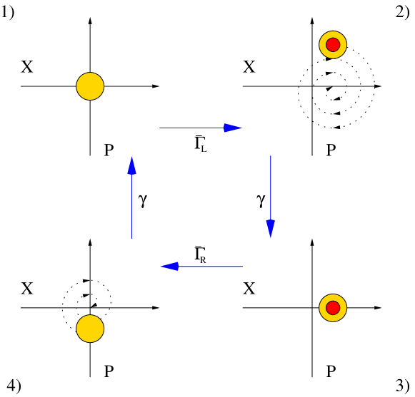
Refer to caption
Figure 6.1: Schematic picture of the tunneling regime. In the scheme we represent the motion of quantum dot in the phase space of the oscillator (position X𝑋X and momentum P𝑃P) and at the same time we keep track of the charge degree of freedom. The four steps on the cycle are described in detail in the text.
  1. 1.

    The dot is empty and in its mechanical ground state. We represent it in the phase space at rest in the origin and neglect in this simplified description the quantum indetermination and/or thermal noise that would blur the mechanical phase space distribution.

  2. 2.

    A tunneling event (from the source lead) and consequent electrostatic force e𝑒e\mathcal{E} perturbs the mechanical state of the dot which gets a positive position and momentum and starts to oscillate due to the harmonic restoring forces. The amplitude of the dot oscillations diminishes due to the dissipative environment. The 1)2)1)\to 2) transition takes place randomly but with a defined rate Γ¯Lsubscript¯Γ𝐿\bar{\Gamma}_{L}: the average injection rate111In the choice of Γ¯Lsubscript¯Γ𝐿\bar{\Gamma}_{L} as injection rate implies that we are taking into account the average occupation of the dot. In other words we are treating the stationary state. See the next chapter for more details..

  3. 3.

    The dot is at rest in the charged state equilibrium position (d=emω2𝑑𝑒𝑚superscript𝜔2d=\frac{e\mathcal{E}}{m\omega^{2}}) given by the combination of the harmonic potential and the electrostatic force. The transition 2)3)2)\to 3) takes place in the short relaxation time 1/γ1𝛾1/\gamma.

  4. 4.

    A second tunnelling event (now towards the drain lead) brings back the dot into the original harmonic potential. The empty dot (distribution function) spirals towards the origin of the phase space and the cycle is closed. The time scale of the 3)4)3)\to 4) transition is given by the inverse ejection rate 1/Γ¯R1subscript¯Γ𝑅1/\bar{\Gamma}_{R} while the mechanical relaxation 4)1)4)\to 1) takes place within a time 1/γ1𝛾1/\gamma.

Since the mechanical damping rate is much larger than the average injection (ejection) rate the system will stay most of the time in the configuration 1 and 3. A description with a coarse grained time do not see the mechanical transients 2 and 3 and is given in terms of a two state model: empty dot in the origin and charged dot in the shifted equilibrium position.

6.2 Shuttling

The shuttling regime is characterized by a non-adiabatic interplay between electrical and mechanical degrees of freedom of the device. In particular the average injection and ejection rate exactly matches the mechanical frequency of the oscillator. The mechanical relaxation rate is much smaller than the mechanical frequency:

γω2π=Γ¯much-less-than𝛾𝜔2𝜋¯Γ\gamma\ll\frac{\omega}{2\pi}=\bar{\Gamma} (6.2)

In the shuttling regime the quantum dot oscillates in a self-sustained stable limit cycle: all the energy pumped per cycle into the system by the electrostatic force is dissipated in the environment during the oscillation itself. Also the shuttling regime can be described by a four step cycle (see Fig. 6.2):

  1. 1.

    The quantum dot, close to the source lead, is charged with an extra electron. The Coulomb blockade prevents any other charging event. The high chemical potential on the left lead makes the charging incoherent and irreversible.

  2. 2.

    Under the combined effect of the mechanical restoring force and the electrostatic force the dot is accelerated towards the right lead. The tunneling parameters have been chosen such that the dot is effectively decoupled from the left and right lead while close to the center of the oscillation. Thus the electrical state of the device remains unchanged along most of the oscillation trajectory.

  3. 3.

    The dot is close to the right lead and the very high ejection rate makes the electron unloading practically deterministic.

  4. 4.

    The empty dot returns towards the left lead under the action of the restoring force of the harmonic oscillator and completes the cycle.

This sequential “classical” description of the shuttling regime is motivated by the phase space analysis of the previous chapter. The current saturation of one electron per cycle and the low noise seem to confirm this interpretation. At least for the most classical parameters range we will see that the dynamics is well described by a “trajectory” in the phase space of the system where a mean field charge coordinate has been added to the mechanical position and momentum222See section 7.2 .
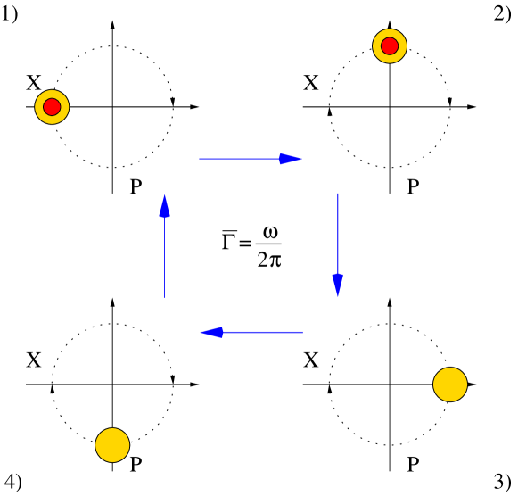
Refer to caption
Figure 6.2: Schematic picture of the shuttling regime.

6.3 Coexistence

At intermediate damping rates the shuttle device shows bistability. Under these conditions neither the tunneling or the shuttling are globally stable regimes and the noise present in the system (shot noise of the charge transfer, thermal noise, quantum mechanical indetermination) causes the random switching between the two processes. The bistability is represented in the stationary distribution function by the coexisting tunneling and shuttling features. We showed that tunneling and shuttling regimes are associated with different average currents. It is not difficult to imagine that the current of the coexistence regime is an average of the shuttling and tunneling currents weighted on the probability for the device to be in one or in the other regime. The slow switching between these two currents generates the peculiar huge super-poissonian Fano factor that also characterized the coexistence regime. It is possible to demonstrate that the zero frequency current noise associated to a slow dichotomous switching between two states with average currents I+subscript𝐼I_{+} and Isubscript𝐼I_{-} reads:

S(0)=αβ(α+β)3(I+I)2𝑆0𝛼𝛽superscript𝛼𝛽3superscriptsubscript𝐼subscript𝐼2S(0)=\frac{\alpha\beta}{(\alpha+\beta)^{3}}(I_{+}-I_{-})^{2} (6.3)

where α𝛼\alpha (β𝛽\beta) is the switching rate from state 1 to 2 (2 to 1). It is important that the average transition time between shuttling and tunneling is the longest time scale in the system dynamics. This fact ensures:

  1. 1.

    Many tunneling or shuttling events before the regime transition take place and thus there exists a well defined average current for the two “states”;

  2. 2.

    A huge Fano factor FIsh/α𝐹subscript𝐼𝑠𝛼F\approx I_{sh}/\alpha.

The time resolved dynamics for the coexistence regime is depicted in figure 6.3 where the transition rates between the two regime are represented respectively by ΓoutsubscriptΓ𝑜𝑢𝑡\Gamma_{out} (tunneling \to shuttling) and ΓinsubscriptΓ𝑖𝑛\Gamma_{in} (shuttling \to tunneling). The names (in𝑖𝑛in and out𝑜𝑢𝑡out) associated to the transition rates are motivated by the dynamics of the mechanical amplitude during the transition. The average oscillation amplitude are very different in the shuttling and tunneling regime and can be used to identify the two states. In fact we will describe the switching dynamics in terms of a bistable potential with the amplitude as the effective coordinate333See section 7.3 for details..
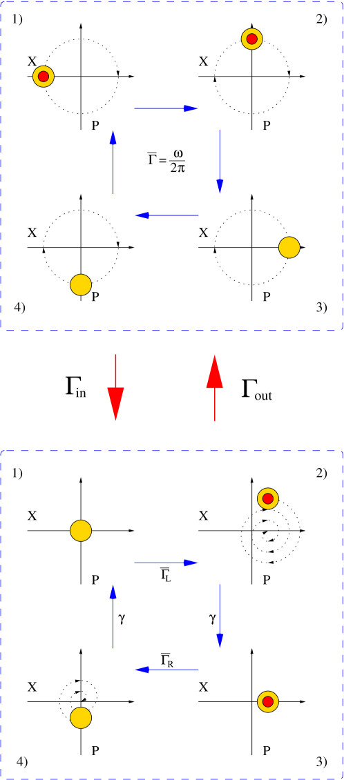
Refer to caption
Figure 6.3: Schematic picture of the coexistence regime.

Chapter 7 Simplified models

We qualitatively described in the previous chapter three possible operating regimes for shuttle-devices. They represent for the SDQS the whole scenario of possible dynamics. Part of the complexity of the TDQS is also captured in this scheme111For a further insight into this particular model see [7, 12, 33].. The specific separation of time scales allows us to identify the relevant variables and describe each regime by a specific simplified model. Models for the tunneling, shuttling and coexistence regime are analyzed separately in the three following sections. We also give a comparison with the full description in terms of Wigner distributions, current and current-noise to prove that the models, at least in the limits set by the chosen investigation tools, capture the relevant dynamics.

7.1 Renormalized resonant tunneling

The electrical dynamics is definitely the slowest in the tunneling regime since the mechanical relaxation time (much longer in itself than the oscillation period) is much shorter than the average injection or ejection time. We already noticed (sec. 6.1) that, because of this time-scale separation, the observation of the device dynamics would most of the time show two mechanically frozen states:

0.

Empty dot at rest in the oscillator equilibrium position

1.

Charged dot in the shifted equilibrium position of the harmonic oscillator perturbed by the constant electrostatic force e𝑒e\mathcal{E}.

We combine this observation with a quantum description of the mechanical oscillator and possible thermal noise under the assumption that the n𝑛n-resolved reduced density matrix of the device can be written in the form:

σ00(n)(t)=p00(n)(t)σth(0)σ11(n)(t)=p11(n)(t)σth(e)superscriptsubscript𝜎00𝑛𝑡subscriptsuperscript𝑝𝑛00𝑡subscript𝜎th0superscriptsubscript𝜎11𝑛𝑡subscriptsuperscript𝑝𝑛11𝑡subscript𝜎th𝑒\begin{split}\sigma_{00}^{(n)}(t)&=p^{(n)}_{00}(t)\sigma_{\rm th}(0)\\ \sigma_{11}^{(n)}(t)&=p^{(n)}_{11}(t)\sigma_{\rm th}(e\mathcal{E})\end{split} (7.1)

where

σth()=eβ(Hoscx)Trosc[eβ(Hoscx)]subscript𝜎thsuperscript𝑒𝛽subscript𝐻osc𝑥subscriptTroscdelimited-[]superscript𝑒𝛽subscript𝐻osc𝑥\sigma_{\rm th}(\mathcal{F})=\frac{e^{-\beta(H_{\rm osc}-\mathcal{F}x)}}{{\rm Tr}_{\rm osc}\left[e^{-\beta(H_{\rm osc}-\mathcal{F}x)}\right]} (7.2)

is the thermal density matrix of a harmonic oscillator subject to an external force \mathcal{F}. The functions p00(n)(t)subscriptsuperscript𝑝𝑛00𝑡p^{(n)}_{00}(t) and p11(n)(t)subscriptsuperscript𝑝𝑛11𝑡p^{(n)}_{11}(t) represent the probability to find the system respectively in the state 0 or 1 that we described above when n𝑛n electrons have tunnelled through the dot. The sum over all possible device and bath configurations is np00(n)(t)+p11(n)(t)=1subscript𝑛subscriptsuperscript𝑝𝑛00𝑡subscriptsuperscript𝑝𝑛11𝑡1\sum_{n}p^{(n)}_{00}(t)+p^{(n)}_{11}(t)=1 at all times. The equations of motion for the probabilities pii(n)(t)subscriptsuperscript𝑝𝑛𝑖𝑖𝑡p^{(n)}_{ii}(t) can be derived by inserting the assumption (7.1) in the n𝑛n-GME (3.98) and taking the trace over the mechanical degrees of freedom222The damping Liouvillean dampsubscriptdamp\mathcal{L}_{\rm damp} is missing in 3.98. Anyway, together with the coherent Liouvillean cohsubscriptcoh\mathcal{L}_{\rm coh}, it does not contribute to the equation of motion for the pii(n)subscriptsuperscript𝑝𝑛𝑖𝑖p^{(n)}_{ii}. They vanish under the trace TroscsubscriptTrosc{\rm Tr}_{\rm osc} because of their commutator structure.:

p˙00(n)=Γ~Rp11(n1)Γ~Lp00(n)p˙11(n)=Γ~Lp00(n)Γ~Rp11(n)subscriptsuperscript˙𝑝𝑛00subscript~Γ𝑅subscriptsuperscript𝑝𝑛111subscript~Γ𝐿subscriptsuperscript𝑝𝑛00subscriptsuperscript˙𝑝𝑛11subscript~Γ𝐿subscriptsuperscript𝑝𝑛00subscript~Γ𝑅subscriptsuperscript𝑝𝑛11\begin{split}\dot{p}^{(n)}_{00}&=\tilde{\Gamma}_{R}\,p^{(n-1)}_{11}-\tilde{\Gamma}_{L}\,p^{(n)}_{00}\\ \dot{p}^{(n)}_{11}&=\tilde{\Gamma}_{L}\,p^{(n)}_{00}-\tilde{\Gamma}_{R}\,p^{(n)}_{11}\end{split} (7.3)

where

Γ~L=Trosc[ΓLe2xλσth(0)]Γ~R=Trosc[ΓRe2xλσth(e)]subscript~Γ𝐿subscriptTroscdelimited-[]subscriptΓ𝐿superscript𝑒2𝑥𝜆subscript𝜎th0subscript~Γ𝑅subscriptTroscdelimited-[]subscriptΓ𝑅superscript𝑒2𝑥𝜆subscript𝜎th𝑒\begin{split}\tilde{\Gamma}_{L}&={\rm Tr}_{\rm osc}\left[\Gamma_{L}e^{-\frac{2x}{\lambda}}\sigma_{\rm th}(0)\right]\\ \tilde{\Gamma}_{R}&={\rm Tr}_{\rm osc}\left[\Gamma_{R}e^{\frac{2x}{\lambda}}\sigma_{\rm th}(e\mathcal{E})\right]\end{split} (7.4)

are the injection and ejection rates renormalized to take into account the quantum/thermal distribution of the harmonic oscillator position. The master equation (7.3) summed over the number n𝑛n of electrons collected in the right lead reads:

p˙00=Γ~Rp11Γ~Lp00p˙11=Γ~Lp00Γ~Rp11subscript˙𝑝00subscript~Γ𝑅subscript𝑝11subscript~Γ𝐿subscript𝑝00subscript˙𝑝11subscript~Γ𝐿subscript𝑝00subscript~Γ𝑅subscript𝑝11\begin{split}\dot{p}_{00}&=\tilde{\Gamma}_{R}\,p_{11}-\tilde{\Gamma}_{L}\,p_{00}\\ \dot{p}_{11}&=\tilde{\Gamma}_{L}\,p_{00}-\tilde{\Gamma}_{R}\,p_{11}\end{split} (7.5)

where we have introduced the occupation probabilities of the state i𝑖i piin=0pii(n)subscript𝑝𝑖𝑖superscriptsubscript𝑛0superscriptsubscript𝑝𝑖𝑖𝑛p_{ii}\equiv\sum_{n=0}^{\infty}p_{ii}^{(n)}. Equations (7.5) describe the dynamics of a resonant tunneling device. The effects of the movable grain are contained in the effective rates Γ~L,Γ~Rsubscript~Γ𝐿subscript~Γ𝑅\tilde{\Gamma}_{L},\tilde{\Gamma}_{R}.

7.1.1 Electrical rates

The renormalized electrical rates can be calculated analytically as functions of the model parameters. The calculation gives the exact contribution of the quantum mechanical and thermal noise to the electrical dynamics. We first consider the limit of very low temperatures kBTωmuch-less-thansubscript𝑘𝐵𝑇Planck-constant-over-2-pi𝜔k_{B}T\ll\hbar\omega. Only the ground state of the harmonic oscillator is occupied and the renormalized injection rate reads:

Γ~L=Trosc[|00|ΓLe2x/λ]=ΓL0|e2xλ|0=ΓLπ+𝑑ξexp[(ξ2+2ξx0λ)]=ΓLe(x0λ)2subscript~Γ𝐿subscriptTroscdelimited-[]ket0bra0subscriptΓ𝐿superscript𝑒2𝑥𝜆subscriptΓ𝐿quantum-operator-product0superscript𝑒2𝑥𝜆0subscriptΓ𝐿𝜋superscriptsubscriptdifferential-d𝜉superscript𝜉22𝜉subscript𝑥0𝜆subscriptΓ𝐿superscript𝑒superscriptsubscript𝑥0𝜆2\begin{split}\tilde{\Gamma}_{L}&={\rm Tr}_{\rm osc}\left[|0\rangle\!\langle 0|\Gamma_{L}e^{-2x/\lambda}\right]=\Gamma_{L}\langle 0|e^{-\frac{2x}{\lambda}}|0\rangle\\ &=\frac{\Gamma_{L}}{\sqrt{\pi}}\int_{-\infty}^{+\infty}d\xi\,\exp\left[-\left(\xi^{2}+\frac{2\xi x_{0}}{\lambda}\right)\right]=\Gamma_{L}e^{(\frac{x_{0}}{\lambda})^{2}}\end{split} (7.6)

where |0ket0|0\rangle is the vector representing the ground state of the harmonic oscillator and x0=/(mω)subscript𝑥0Planck-constant-over-2-pi𝑚𝜔x_{0}=\sqrt{\hbar/(m\omega)}. For the calculation of the renormalized ejection rate it is useful to introduce the displacement unitary operator:

D(l)=eilp𝐷𝑙superscript𝑒𝑖Planck-constant-over-2-pi𝑙𝑝D(l)=e^{-\frac{i}{\hbar}lp} (7.7)

with the properties333These properties can be easily derived from the definition of the operator D(l)𝐷𝑙D(l) and the Baker-Hausdorff-Campbell formula [25].:

D(l)dD(l)=dlmω2D(l)dD(l)=dlmω2D(l)xD(l)=xl𝐷𝑙𝑑superscript𝐷𝑙𝑑𝑙𝑚𝜔2Planck-constant-over-2-pi𝐷𝑙superscript𝑑superscript𝐷𝑙superscript𝑑𝑙𝑚𝜔2Planck-constant-over-2-pi𝐷𝑙𝑥superscript𝐷𝑙𝑥𝑙\begin{split}D(l)dD^{{\dagger}}(l)&=d-l\sqrt{{\textstyle\frac{m\omega}{2\hbar}}}\\ D(l)d^{{\dagger}}D^{{\dagger}}(l)&=d^{{\dagger}}-l\sqrt{{\textstyle\frac{m\omega}{2\hbar}}}\\ D(l)xD^{{\dagger}}(l)&=x-l\end{split} (7.8)

where x,p𝑥𝑝x,p are the position and momentum operators and d,dsuperscript𝑑𝑑d^{{\dagger}},d are the creation and annihilation operators for the harmonic oscillator. In terms of the displacement operator D𝐷D the density matrix σth()subscript𝜎th\sigma_{\rm th}(\mathcal{F}) can be written:

σth()=D(mω2)σth(0)D(mω2)subscript𝜎th𝐷𝑚superscript𝜔2subscript𝜎th0superscript𝐷𝑚superscript𝜔2\sigma_{\rm th}(\mathcal{F})=D\left({\textstyle\frac{\mathcal{F}}{m\omega^{2}}}\right)\sigma_{\rm th}(0)D^{{\dagger}}\left({\textstyle\frac{\mathcal{F}}{m\omega^{2}}}\right) (7.9)

Only the displaced ground state contributes to the renormalized ejection rate:

Γ~R=Trosc[D(d)|00|D(d)ΓRe2x/λ]=ΓR0|D(d)e2xλD(d)|0=ΓRe2dλ0|e2xλ|0=ΓRe2dλ+(x0λ)2subscript~Γ𝑅subscriptTroscdelimited-[]𝐷𝑑ket0bra0superscript𝐷𝑑subscriptΓ𝑅superscript𝑒2𝑥𝜆subscriptΓ𝑅quantum-operator-product0superscript𝐷𝑑superscript𝑒2𝑥𝜆𝐷𝑑0subscriptΓ𝑅superscript𝑒2𝑑𝜆quantum-operator-product0superscript𝑒2𝑥𝜆0subscriptΓ𝑅superscript𝑒2𝑑𝜆superscriptsubscript𝑥0𝜆2\begin{split}\tilde{\Gamma}_{R}&={\rm Tr}_{\rm osc}\left[D(d)|0\rangle\!\langle 0|D^{{\dagger}}(d)\,\Gamma_{R}e^{-2x/\lambda}\right]\\ &=\Gamma_{R}\langle 0|D^{{\dagger}}(d)\,e^{\frac{2x}{\lambda}}\,D(d)|0\rangle\\ &=\Gamma_{R}e^{\frac{2d}{\lambda}}\langle 0|e^{\frac{2x}{\lambda}}|0\rangle=\Gamma_{R}e^{\frac{2d}{\lambda}+\left(\frac{x_{0}}{\lambda}\right)^{2}}\end{split} (7.10)

where d=emω2𝑑𝑒𝑚superscript𝜔2d=\frac{e\mathcal{E}}{m\omega^{2}}.

As expected the ejection rate is modified by the “classical” shift d𝑑d of the equilibrium position due to the electrostatic force on the charged dot. Somehow unexpectedly both rates are also enhanced by the quantum uncertainty in the position present in the oscillator ground state. The relevance of the quantum correction is given by the ratio between the zero point position dispersion x0subscript𝑥0x_{0} and the tunneling length λ𝜆\lambda: the smaller the ratio the smaller the correction.

The calculation of the finite temperature rates is problematic due to the presence in the trace of the product of the exponentials of two non commutative operators (Hosc,xsubscript𝐻osc𝑥H_{\rm osc},x). We solve the problem using the low temperature calculation just performed and some symmetry arguments. First we notice that the density matrix σthsubscript𝜎th\sigma_{\rm th} is the stationary solution of the GME444We have assumed this property from the very beginning. For a detailed proof of this statement see for example “The Theory of Open Quantum Systems” by H.-P. Breuer and F. Petruccione [46].:

σ˙=i[Hosc,σ]iγ2[x,{p,σ}]γmω[nB(ω)+12][x,[x,σ]]˙𝜎𝑖Planck-constant-over-2-pisubscript𝐻osc𝜎𝑖𝛾2Planck-constant-over-2-pi𝑥𝑝𝜎𝛾𝑚𝜔Planck-constant-over-2-pidelimited-[]subscript𝑛𝐵𝜔12𝑥𝑥𝜎\dot{\sigma}=-\frac{i}{\hbar}[H_{\rm osc},\sigma]-\frac{i\gamma}{2\hbar}[x,\{p,\sigma\}]-\frac{\gamma m\omega}{\hbar}\left[n_{B}(\omega)+\frac{1}{2}\right][x,[x,\sigma]] (7.11)

We express the trace in the position (generalized) basis |qket𝑞|q\rangle and the renormalized rates take the form:

Γ~L=ΓL𝑑qPth(q)e2qλΓ~R=ΓRe2dλ𝑑qPth(q)e2qλsubscript~Γ𝐿subscriptΓ𝐿differential-d𝑞subscript𝑃th𝑞superscript𝑒2𝑞𝜆subscript~Γ𝑅subscriptΓ𝑅superscript𝑒2𝑑𝜆differential-d𝑞subscript𝑃th𝑞superscript𝑒2𝑞𝜆\begin{split}\tilde{\Gamma}_{L}&=\Gamma_{L}\int dq\,P_{\rm th}(q)e^{-\frac{2q}{\lambda}}\\ \tilde{\Gamma}_{R}&=\Gamma_{R}e^{\frac{2d}{\lambda}}\int dq\,P_{\rm th}(q)e^{\frac{2q}{\lambda}}\end{split} (7.12)

where we have introduced the coordinate probability distribution Pth(q)q|σth|qsubscript𝑃th𝑞quantum-operator-product𝑞subscript𝜎th𝑞P_{\rm th}(q)\equiv\langle q|\sigma_{\rm th}|q\rangle. We encountered this distribution already in section (4.1) in the axiomatical definition of the Wigner function. We required specifically:

𝑑pW(q,p,t)=q|σ|qdifferential-d𝑝𝑊𝑞𝑝𝑡quantum-operator-product𝑞𝜎𝑞\int dpW(q,p,t)=\langle q|\sigma|q\rangle (7.13)

The problem is thus shifted to the calculation of the Wigner function associated with the thermal density matrix σthsubscript𝜎th\sigma_{\rm th}. The dynamics of the Wigner distribution is given by the Fokker-Planck equation555The Klein-Kramers equations of second order are also called Fokker-Plank equations. related to the GME (7.11):

Wτ=[XPPX+γωP(P+P)]W𝑊𝜏delimited-[]𝑋𝑃𝑃𝑋𝛾𝜔𝑃𝑃𝑃𝑊\frac{\partial W}{\partial\tau}=\left[X\frac{\partial}{\partial P}-P\frac{\partial}{\partial X}+\frac{\gamma}{\omega}\frac{\partial}{\partial P}\left(P+\frac{\partial}{\partial P}\right)\right]\,W (7.14)

where we have defined the adimensional variables:

τ=ωt,X=q,P=pmωformulae-sequence𝜏𝜔𝑡formulae-sequence𝑋𝑞𝑃𝑝𝑚𝜔\tau=\omega t,\quad X=\frac{q}{\ell},\quad P=\frac{p}{m\omega\ell} (7.15)

and =2mω(2nB+1)Planck-constant-over-2-pi2𝑚𝜔2subscript𝑛𝐵1\ell=\sqrt{\frac{\hbar}{2m\omega}(2n_{B}+1)}. The Fokker-Planck equation (7.14) does not depend on the temperature. The stationary solution is the Gaussian666This statement can be easily verified by substitution. In order to derive it one considers that the Gaussian in P𝑃P is the solution for the dissipative part of the Liouvillean (proportional to γ𝛾\gamma) while the coherent part is solved by spherically symmetric distributions since in polar coordinates (A,ϕ)𝐴italic-ϕ(A,\phi) we have XPPXϕ𝑋subscript𝑃𝑃subscript𝑋subscriptitalic-ϕX\partial_{P}-P\partial_{X}\to-\partial_{\phi}. in X𝑋X and P𝑃P

Wstat(X,P)=12πexp(X2+P22)superscript𝑊stat𝑋𝑃12𝜋superscript𝑋2superscript𝑃22W^{\rm stat}(X,P)=\frac{1}{2\pi}\exp\left(-\frac{X^{2}+P^{2}}{2}\right) (7.16)

with no parameters. The position distribution function Pth(q)subscript𝑃th𝑞P_{\rm th}(q) thus depends on the temperature only in the scaling factor and has the same functional form (Gaussian) of the zero temperature case:

Pth(q)=12π2exp(q222)subscript𝑃th𝑞12𝜋superscript2superscript𝑞22superscript2P_{\rm th}(q)=\frac{1}{\sqrt{2\pi\ell^{2}}}\exp\left(-\frac{q^{2}}{2\ell^{2}}\right) (7.17)

Finally we insert (7.17) into (7.12) and perform the gaussian integrals to obtain the finite temperature rates:

Γ~L=ΓLe2(λ)2Γ~R=ΓRe2dλ+2(λ)2subscript~Γ𝐿subscriptΓ𝐿superscript𝑒2superscript𝜆2subscript~Γ𝑅subscriptΓ𝑅superscript𝑒2𝑑𝜆2superscript𝜆2\begin{split}\tilde{\Gamma}_{L}&=\Gamma_{L}e^{2\left(\frac{\ell}{\lambda}\right)^{2}}\\ \tilde{\Gamma}_{R}&=\Gamma_{R}e^{\frac{2d}{\lambda}+2\left(\frac{\ell}{\lambda}\right)^{2}}\end{split} (7.18)

In the low temperature limit equations (7.18) obviously reduce to (7.6) and (7.10). The high temperature limit kBTωmuch-greater-thansubscript𝑘𝐵𝑇Planck-constant-over-2-pi𝜔k_{B}T\gg\hbar\omega is also interesting:

Γ~L=ΓLe2(λthλ)2Γ~R=ΓRe2dλ+2(λthλ)2subscript~Γ𝐿subscriptΓ𝐿superscript𝑒2superscriptsubscript𝜆th𝜆2subscript~Γ𝑅subscriptΓ𝑅superscript𝑒2𝑑𝜆2superscriptsubscript𝜆th𝜆2\begin{split}\tilde{\Gamma}_{L}&=\Gamma_{L}e^{2\left(\frac{\lambda_{\rm th}}{\lambda}\right)^{2}}\\ \tilde{\Gamma}_{R}&=\Gamma_{R}e^{\frac{2d}{\lambda}+2\left(\frac{\lambda_{\rm th}}{\lambda}\right)^{2}}\end{split} (7.19)

In this case the renormalization is the more effective the larger is the thermal length λth=kBT/(mω2)subscript𝜆thsubscript𝑘𝐵𝑇𝑚superscript𝜔2\lambda_{\rm th}=\sqrt{k_{B}T/(m\omega^{2})} compared to the tunneling length λ𝜆\lambda.

7.1.2 Phase-space distribution

The phase space distribution for the stationary state of the simplified model for the tunneling regime is built on the Wigner representation of the thermal density matrix σthsubscript𝜎th\sigma_{\rm th} and the stationary solution of the system (7.5) for the occupation piisubscript𝑝𝑖𝑖p_{ii} of the electromechanical states i𝑖i. The latter is easily expressed in terms of the renormalized rates Γ~L,Rsubscript~Γ𝐿𝑅\tilde{\Gamma}_{L,R}:

p00stat=Γ~RΓ~L+Γ~Rp11stat=Γ~LΓ~L+Γ~Rsuperscriptsubscript𝑝00statsubscript~Γ𝑅subscript~Γ𝐿subscript~Γ𝑅superscriptsubscript𝑝11statsubscript~Γ𝐿subscript~Γ𝐿subscript~Γ𝑅\begin{split}p_{00}^{\rm stat}&=\frac{\tilde{\Gamma}_{R}}{\tilde{\Gamma}_{L}+\tilde{\Gamma}_{R}}\\ p_{11}^{\rm stat}&=\frac{\tilde{\Gamma}_{L}}{\tilde{\Gamma}_{L}+\tilde{\Gamma}_{R}}\end{split} (7.20)

We have already met the Wigner distribution corresponding to the thermal density matrix σthsubscript𝜎th\sigma_{\rm th} in Eq. (7.16). We now rewrite it in terms of the canonical variables (q,p)𝑞𝑝(q,p):

σth(0)Wth(q,p)=12πmω2exp{12[(q)2+(pmω)2]}subscript𝜎th0subscript𝑊th𝑞𝑝12𝜋𝑚𝜔superscript212delimited-[]superscript𝑞2superscript𝑝𝑚𝜔2\sigma_{\rm th}(0)\to W_{\rm th}(q,p)=\frac{1}{2\pi m\omega\ell^{2}}\exp\left\{-\frac{1}{2}\left[\left(\frac{q}{\ell}\right)^{2}+\left(\frac{p}{\ell m\omega}\right)^{2}\right]\right\} (7.21)

The calculation of the Wigner function for the displaced thermal distribution σth(e)subscript𝜎th𝑒\sigma_{\rm th}(e\mathcal{E}) can be performed using the properties of the displacement operators D𝐷D:

σth(e)12π𝑑ξqξ2|D(d)σth(0)D(d)|q+ξ2exp(ipξ)=12π𝑑ξqdξ2|σth(0)|qd+ξ2exp(ipξ)=Wth(qd,p)subscript𝜎th𝑒12𝜋Planck-constant-over-2-pidifferential-d𝜉quantum-operator-product𝑞𝜉2𝐷𝑑subscript𝜎th0superscript𝐷𝑑𝑞𝜉2𝑖Planck-constant-over-2-pi𝑝𝜉12𝜋Planck-constant-over-2-pidifferential-d𝜉quantum-operator-product𝑞𝑑𝜉2subscript𝜎th0𝑞𝑑𝜉2𝑖Planck-constant-over-2-pi𝑝𝜉subscript𝑊th𝑞𝑑𝑝\begin{split}\sigma_{\rm th}(e\mathcal{E})&\to\frac{1}{2\pi\hbar}\int d\xi\left\langle q-\frac{\xi}{2}\right|D(d)\sigma_{\rm th}(0)D^{{\dagger}}(d)\left|q+\frac{\xi}{2}\right\rangle\exp\left(\frac{i}{\hbar}p\xi\right)\\ &=\frac{1}{2\pi\hbar}\int d\xi\left\langle q-d-\frac{\xi}{2}\right|\sigma_{\rm th}(0)\left|q-d+\frac{\xi}{2}\right\rangle\exp\left(\frac{i}{\hbar}p\xi\right)\\ &=W_{\rm th}(q-d,p)\end{split} (7.22)

where we have used the property D(l)|a=|al𝐷𝑙ket𝑎ket𝑎𝑙D(l)|a\rangle=|a-l\rangle that we can be proven as follows: given |aket𝑎|a\rangle eigenvector for the position operator x𝑥x with eigenvalue a𝑎a

xD(l)|a=D(l)D(l)xD(l)|a=D(l)(xl)|a=(al)D(l)|a𝑥𝐷𝑙ket𝑎𝐷𝑙superscript𝐷𝑙𝑥𝐷𝑙ket𝑎𝐷𝑙𝑥𝑙ket𝑎𝑎𝑙𝐷𝑙ket𝑎\begin{split}xD(l)|a\rangle&=D(l)\,D^{{\dagger}}(l)\,x\,D(l)|a\rangle\\ &=D(l)(x-l)|a\rangle=(a-l)D(l)|a\rangle\end{split} (7.23)

The stationary solution of the Klein-Kramers equation (4.32) in the tunneling regime limit thus reads:

W00stat(q,p)=Γ~RΓ~L+Γ~RWth(q,p)W11stat(q,p)=Γ~LΓ~L+Γ~RWth(qd,p)superscriptsubscript𝑊00stat𝑞𝑝subscript~Γ𝑅subscript~Γ𝐿subscript~Γ𝑅subscript𝑊th𝑞𝑝superscriptsubscript𝑊11stat𝑞𝑝subscript~Γ𝐿subscript~Γ𝐿subscript~Γ𝑅subscript𝑊th𝑞𝑑𝑝\begin{split}W_{00}^{\rm stat}(q,p)&=\frac{\tilde{\Gamma}_{R}}{\tilde{\Gamma}_{L}+\tilde{\Gamma}_{R}}W_{\rm th}(q,p)\\ W_{11}^{\rm stat}(q,p)&=\frac{\tilde{\Gamma}_{L}}{\tilde{\Gamma}_{L}+\tilde{\Gamma}_{R}}W_{\rm th}(q-d,p)\end{split} (7.24)
Refer to caption
Figure 7.1: Wigner distribution functions for the SDQS in the tunneling regime. calculated numerically using the full description. Coordinates (horizontal axis) are measured in terms of x0subscript𝑥0x_{0}, momenta (vertical axis) in terms of mωx0𝑚𝜔subscript𝑥0m\omega x_{0}. The crosses indicates the cuts in the phase space along which we perform the comparison between numerical and analytical solution shown in figure 7.2. The parameters are: ΓL=ΓR=0.01ωsubscriptΓ𝐿subscriptΓ𝑅0.01𝜔\Gamma_{L}=\Gamma_{R}=0.01\omega, γ=0.25ω𝛾0.25𝜔\gamma=0.25\omega, d=0.5x0𝑑0.5subscript𝑥0d=0.5x_{0}, λ=2x0𝜆2subscript𝑥0\lambda=2x_{0}, T=0𝑇0T=0.
Refer to caption
Figure 7.2: Comparison between the numerical and the analytical results for the Wigner distribution functions. The squares (circles) are numerical results for the parameters mentioned in figure 7.1 in the charged (empty) dot configuration, and the full lines represent the analytical calculations. We also plotted with dots the numerical results for Γ=0.001ωΓ0.001𝜔\Gamma=0.001\omega.

The stationary distribution of the tunneling model is completely determined by the length \ell and associated momentum mω𝑚𝜔m\omega\ell, the equilibrium position shift d𝑑d and the tunneling length λ𝜆\lambda. The electronic and mechanical relaxation rates γ𝛾\gamma and ΓL,RsubscriptΓ𝐿𝑅\Gamma_{L,R} drop out from the solution and only set the range of applicability of the simplified model.

In figures 7.1, 7.2 and 7.3 we compare the Wigner functions calculated both analytically and numerically in the tunneling regime. They show in general a very good agreement. In particular we notice in Fig. 7.2 that the convergence to the tunneling regime is not yet complete for γ=0.25ω𝛾0.25𝜔\gamma=0.25\omega and ΓL,R=0.01ωsubscriptΓ𝐿𝑅0.01𝜔\Gamma_{L,R}=0.01\omega. To check the theory we diminished the bare electrical rate further (the quantum corrections are negligible since λ=2x0𝜆2subscript𝑥0\lambda=2x_{0}, the classical shift can be taken into account and gives a factor e2.7𝑒2.7e\approx 2.7 which does not change the analysis) and kept the mechanical damping fixed to “maintain” the condition γωmuch-less-than𝛾𝜔\gamma\ll\omega. For Γ=0.001ωΓ0.001𝜔\Gamma=0.001\omega we got perfect agreement. We also analyze the temperature dependence of the stationary Wigner function distribution (Fig. 7.3) and verify the scaling given by the temperature dependent length \ell.

Refer to caption
Figure 7.3: Tunneling Wigner distributions as a function of the temperature. The relevant parameters are: γ=0.25ω𝛾0.25𝜔\gamma=0.25\omega, Γ=0.001ωΓ0.001𝜔\Gamma=0.001\omega, nB=0,0.75,1.5subscript𝑛𝐵00.751.5n_{B}=0,0.75,1.5 respectively represented by dots, circles and asterisks. Full lines are the analytical results. See Fig: 7.1 for the other parameters and the scales.

7.1.3 Current

The current through the SDQS towards the right lead is given by the general formula:

IR(t)=n=0nP˙n(t)subscript𝐼𝑅𝑡superscriptsubscript𝑛0𝑛subscript˙𝑃𝑛𝑡I_{R}(t)=\sum_{n=0}^{\infty}n\dot{P}_{n}(t) (7.25)

In the tunneling limit the probabilities Pn(t)subscript𝑃𝑛𝑡P_{n}(t) are be expressed in terms of pii(n)(t)subscriptsuperscript𝑝𝑛𝑖𝑖𝑡p^{(n)}_{ii}(t) since:

Pn(t)=Trosc[p00(n)(t)σth(0)+p11(n)(t)σth(e)]=p00(n)(t)+p11(n)(t)subscript𝑃𝑛𝑡subscriptTroscdelimited-[]subscriptsuperscript𝑝𝑛00𝑡subscript𝜎th0subscriptsuperscript𝑝𝑛11𝑡subscript𝜎th𝑒superscriptsubscript𝑝00𝑛𝑡superscriptsubscript𝑝11𝑛𝑡P_{n}(t)={\rm Tr}_{\rm osc}[p^{(n)}_{00}(t)\sigma_{\rm th}(0)+p^{(n)}_{11}(t)\sigma_{\rm th}(e\mathcal{E})]=p_{00}^{(n)}(t)+p_{11}^{(n)}(t) (7.26)

Apart from the renormalized electronic rates the system has no sign of the oscillator degree of freedom and can be treated formally as a static quantum dot. We write in complete analogy with (3.54) the right (left) lead time dependent current:

IR(t)=Γ~Rp11(t)IL(t)=Γ~Lp00(t)subscript𝐼𝑅𝑡subscript~Γ𝑅subscript𝑝11𝑡subscript𝐼𝐿𝑡subscript~Γ𝐿subscript𝑝00𝑡\begin{split}I_{R}(t)&=\tilde{\Gamma}_{R}p_{11}(t)\\ I_{L}(t)&=\tilde{\Gamma}_{L}p_{00}(t)\end{split} (7.27)

In the stationary limit they coincide:

Istat=limtIR(t)=Γ~Rp11stat=Γ¯RlimtIL(t)=Γ~Lp00stat=Γ¯L=Γ~RΓ~LΓ~L+Γ~R=Γ¯superscript𝐼statsubscript𝑡subscript𝐼𝑅𝑡subscript~Γ𝑅subscriptsuperscript𝑝stat11subscript¯Γ𝑅missing-subexpressionmissing-subexpressionsubscript𝑡subscript𝐼𝐿𝑡subscript~Γ𝐿subscriptsuperscript𝑝stat00subscript¯Γ𝐿subscript~Γ𝑅subscript~Γ𝐿subscript~Γ𝐿subscript~Γ𝑅¯ΓI^{\rm stat}=\begin{array}[]{c}\nearrow\\ \searrow\end{array}\begin{array}[]{c}\lim_{t\to\infty}I_{R}(t)=\tilde{\Gamma}_{R}p^{\rm stat}_{11}=\bar{\Gamma}_{R}\\ \\ \\ \lim_{t\to\infty}I_{L}(t)=\tilde{\Gamma}_{L}p^{\rm stat}_{00}=\bar{\Gamma}_{L}\end{array}\begin{array}[]{c}\searrow\\ \nearrow\end{array}=\frac{\tilde{\Gamma}_{R}\tilde{\Gamma}_{L}}{\tilde{\Gamma}_{L}+\tilde{\Gamma}_{R}}=\bar{\Gamma} (7.28)

We stress the difference between Γ¯L(R)subscript¯Γ𝐿𝑅\bar{\Gamma}_{L(R)} and Γ~L(R)subscript~Γ𝐿𝑅\tilde{\Gamma}_{L(R)}: while the first is the average injection (ejection rate) and thus represents the current through the device, the second is an average over the mechanical distribution function of the position dependent rate operator. Despite being an average rate it does not take into account the charge state of the dot (and the Coulomb blockade) and thus cannot represent the current through the device. We show in figure 7.4 the current calculated numerically and the asymptotic value of the tunneling regime given by Eq. (7.28).
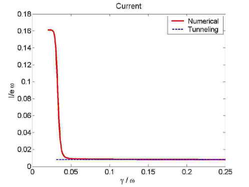
Refer to caption
Figure 7.4: Current as a function of the damping for the SDQS. The asymptotic tunneling limit is indicated. The parameters are: ΓL=ΓR=0.01ωsubscriptΓ𝐿subscriptΓ𝑅0.01𝜔\Gamma_{L}=\Gamma_{R}=0.01\omega, γ=0.25ω𝛾0.25𝜔\gamma=0.25\omega, d=0.5x0𝑑0.5subscript𝑥0d=0.5x_{0}, λ=2x0𝜆2subscript𝑥0\lambda=2x_{0}, T=0𝑇0T=0.

7.1.4 Current-noise

The calculation of the current noise and Fano factor in the tunneling regime is interesting since it gives us the opportunity to explain the concepts and methods we introduced in section 5.3 still keeping a computational level analytically affordable due to the much lesser number of degrees of freedom of the effective model.

We start with the MacDonald formula for the zero frequency current noise:

S(0)=limt+ddt[n=0n2Pn(t)(n=0nPn(t))2]𝑆0subscript𝑡𝑑𝑑𝑡delimited-[]superscriptsubscript𝑛0superscript𝑛2subscript𝑃𝑛𝑡superscriptsuperscriptsubscript𝑛0𝑛subscript𝑃𝑛𝑡2S(0)=\lim_{t\to+\infty}\frac{d}{dt}\Big{[}\sum_{n=0}^{\infty}n^{2}P_{n}(t)-\big{(}\sum_{n=0}^{\infty}nP_{n}(t)\big{)}^{2}\Big{]} (7.29)

where Pn(t)=p00(n)+p11(n)subscript𝑃𝑛𝑡superscriptsubscript𝑝00𝑛superscriptsubscript𝑝11𝑛P_{n}(t)=p_{00}^{(n)}+p_{11}^{(n)} and the equation of motion for pii(n)superscriptsubscript𝑝𝑖𝑖𝑛p_{ii}^{(n)} are:

p˙00(n)=Γ~Rp11(n1)Γ~Lp00(n)p˙11(n)=Γ~Lp00(n)Γ~Rp11(n)subscriptsuperscript˙𝑝𝑛00subscript~Γ𝑅subscriptsuperscript𝑝𝑛111subscript~Γ𝐿subscriptsuperscript𝑝𝑛00subscriptsuperscript˙𝑝𝑛11subscript~Γ𝐿subscriptsuperscript𝑝𝑛00subscript~Γ𝑅subscriptsuperscript𝑝𝑛11\begin{split}\dot{p}^{(n)}_{00}&=\tilde{\Gamma}_{R}\,p^{(n-1)}_{11}-\tilde{\Gamma}_{L}\,p^{(n)}_{00}\\ \dot{p}^{(n)}_{11}&=\tilde{\Gamma}_{L}\,p^{(n)}_{00}-\tilde{\Gamma}_{R}\,p^{(n)}_{11}\end{split} (7.30)

We identify the effective Liouvillean \mathcal{L} for the relevant variables pii(t)subscript𝑝𝑖𝑖𝑡p_{ii}(t) in the model:

=(Γ~LΓ~RΓ~LΓ~R)matrixsubscript~Γ𝐿subscript~Γ𝑅subscript~Γ𝐿subscript~Γ𝑅\mathcal{L}=\begin{pmatrix}-\tilde{\Gamma}_{L}&\tilde{\Gamma}_{R}\\ \tilde{\Gamma}_{L}&-\tilde{\Gamma}_{R}\end{pmatrix} (7.31)

The evaluation of the different terms of the current-noise can be carried out by introducing the generating functions Fii(t;z)=npii(n)(t)znsubscript𝐹𝑖𝑖𝑡𝑧subscript𝑛superscriptsubscript𝑝𝑖𝑖𝑛𝑡superscript𝑧𝑛F_{ii}(t;z)=\sum_{n}p_{ii}^{(n)}(t)z^{n} and following the same reasoning we indicated in section 5.3.2. The result is formally the same777The perfect matching can be better appreciated in a more general super-operator formulation in which the current noise reads in both cases 0~|IR2IR𝒬1𝒬IR|0delimited-⟨⟩quantum-operator-product~0subscript𝐼𝑅2subscript𝐼𝑅𝒬superscript1𝒬subscript𝐼𝑅0\langle\!\langle\tilde{0}|I_{R}-2I_{R}\mathcal{QL}^{-1}\mathcal{Q}I_{R}|0\rangle\!\rangle. See for example [33] for details.: we express the Fano factor in terms of the stationary probabilities piistatsuperscriptsubscript𝑝𝑖𝑖statp_{ii}^{\rm stat} and the pseudoinverse of the the Liouvillean 𝒬1𝒬𝒬superscript1𝒬\mathcal{QL}^{-1}\mathcal{Q}.

F=12Istat(0Γ~R00)𝒬1𝒬(0Γ~R00)(p00statp11stat)1𝐹12superscript𝐼statsubscriptnormmatrix0subscript~Γ𝑅00𝒬superscript1𝒬matrix0subscript~Γ𝑅00matrixsuperscriptsubscript𝑝00statsuperscriptsubscript𝑝11stat1F=1-\frac{2}{I^{\rm stat}}\left\|\begin{pmatrix}0&\tilde{\Gamma}_{R}\\ 0&0\end{pmatrix}\mathcal{QL}^{-1}\mathcal{Q}\begin{pmatrix}0&\tilde{\Gamma}_{R}\\ 0&0\end{pmatrix}\begin{pmatrix}p_{00}^{\rm stat}\\ p_{11}^{\rm stat}\end{pmatrix}\right\|_{1} (7.32)

where 1\|\bullet\|_{1} is the sum of the elements of the vector. The projectors 𝒫𝒫\mathcal{P} and 𝒬𝒬\mathcal{Q}, built from their definition (see sec. 5.3.2), have the matrix form:

𝒫=(p00statp00statp11statp11stat),𝒬=(p11statp00statp11statp00stat).formulae-sequence𝒫matrixsuperscriptsubscript𝑝00statsuperscriptsubscript𝑝00statsuperscriptsubscript𝑝11statsuperscriptsubscript𝑝11stat𝒬matrixsuperscriptsubscript𝑝11statsuperscriptsubscript𝑝00statsuperscriptsubscript𝑝11statsuperscriptsubscript𝑝00stat\mathcal{P}=\begin{pmatrix}p_{00}^{\rm stat}&p_{00}^{\rm stat}\\ p_{11}^{\rm stat}&p_{11}^{\rm stat}\end{pmatrix},\quad\mathcal{Q}=\begin{pmatrix}\phantom{-}p_{11}^{\rm stat}&-p_{00}^{\rm stat}\\ -p_{11}^{\rm stat}&\phantom{-}p_{00}^{\rm stat}\end{pmatrix}. (7.33)

For the explicit calculation of Eq. (7.32) we define the auxiliary vector ΣΣ\Sigma:

Σ=(Σ00Σ11)=𝒬1𝒬(0Γ~R00)(p00statp11stat)ΣmatrixsubscriptΣ00subscriptΣ11𝒬superscript1𝒬matrix0subscript~Γ𝑅00matrixsuperscriptsubscript𝑝00statsuperscriptsubscript𝑝11stat\Sigma=\begin{pmatrix}\Sigma_{00}\\ \Sigma_{11}\end{pmatrix}=\mathcal{QL}^{-1}\mathcal{Q}\begin{pmatrix}0&\tilde{\Gamma}_{R}\\ 0&0\end{pmatrix}\begin{pmatrix}p_{00}^{\rm stat}\\ p_{11}^{\rm stat}\end{pmatrix} (7.34)

that satisfies the equation

Σ=𝒬(0Γ~R00)(p00statp11stat)=Γ~R(p11stat)2(11)Σ𝒬matrix0subscript~Γ𝑅00matrixsuperscriptsubscript𝑝00statsuperscriptsubscript𝑝11statsubscript~Γ𝑅superscriptsuperscriptsubscript𝑝11stat2matrix11\mathcal{L}\Sigma=\mathcal{Q}\begin{pmatrix}0&\tilde{\Gamma}_{R}\\ 0&0\end{pmatrix}\begin{pmatrix}p_{00}^{\rm stat}\\ p_{11}^{\rm stat}\end{pmatrix}=\tilde{\Gamma}_{R}(p_{11}^{\rm stat})^{2}\begin{pmatrix}1\\ -1\end{pmatrix} (7.35)

Together with the condition Σ00+Σ11=0subscriptΣ00subscriptΣ110\Sigma_{00}+\Sigma_{11}=0888This condition is readily proven since the last operator to the left in the definition of ΣΣ\Sigma is 𝒬𝒬\mathcal{Q} and the sum on the elements of ΣΣ\Sigma would extract the component in the direction of the null vector of the Liouvillean. This component has been already projected out by 𝒬𝒬\mathcal{Q}. we can calculate ΣΣ\Sigma and by substitution into (7.32) find the Fano factor F𝐹F:

F=12Γ~RΣ11Istat=12Γ~R(Γ~L+Γ~R)Γ~LΓ~RΓ~RΓ~L2(Γ~L+Γ~R)3=Γ~L2+Γ~R2(Γ~L+Γ~R)2𝐹12subscript~Γ𝑅subscriptΣ11superscript𝐼stat12subscript~Γ𝑅subscript~Γ𝐿subscript~Γ𝑅subscript~Γ𝐿subscript~Γ𝑅subscript~Γ𝑅superscriptsubscript~Γ𝐿2superscriptsubscript~Γ𝐿subscript~Γ𝑅3superscriptsubscript~Γ𝐿2superscriptsubscript~Γ𝑅2superscriptsubscript~Γ𝐿subscript~Γ𝑅2F=1-\frac{2\tilde{\Gamma}_{R}\Sigma_{11}}{I^{\rm stat}}=1-\frac{2\tilde{\Gamma}_{R}(\tilde{\Gamma}_{L}+\tilde{\Gamma}_{R})}{\tilde{\Gamma}_{L}\tilde{\Gamma}_{R}}\frac{\tilde{\Gamma}_{R}\tilde{\Gamma}_{L}^{2}}{(\tilde{\Gamma}_{L}+\tilde{\Gamma}_{R})^{3}}=\frac{\tilde{\Gamma}_{L}^{2}+\tilde{\Gamma}_{R}^{2}}{(\tilde{\Gamma}_{L}+\tilde{\Gamma}_{R})^{2}} (7.36)
Refer to caption
Figure 7.5: Current-noise as a function of the damping for the SDQS. The asymptotic tunneling limit is indicated. The parameters are: ΓL=ΓR=0.01ωsubscriptΓ𝐿subscriptΓ𝑅0.01𝜔\Gamma_{L}=\Gamma_{R}=0.01\omega, γ=0.25ω𝛾0.25𝜔\gamma=0.25\omega, d=0.5x0𝑑0.5subscript𝑥0d=0.5x_{0}, λ=2x0𝜆2subscript𝑥0\lambda=2x_{0}, T=0𝑇0T=0.

7.2 Shuttling: a classical transport regime

The simplified model for the shuttling dynamics is based on the observation –extracted from the full description– that the system exhibits in this operating regime extremely low Fano factors (F102𝐹superscript102F\approx 10^{-2}). In the simplified model we assume that there is no noise at all in the system. Its state is represented by a point that moves on a trajectory in the 3-dimensional device phase-space of position, momentum and charge of the oscillating dot. It is hard not to imagine the charge on the oscillating dot as a stochastic variable governed by tunnelling processes. Nevertheless in the shuttling regime the tunneling events are made effectively deterministic since they are very highly probable at specific times settled by the mechanical dynamics. On the other hand, due to the electrostatic force e𝑒e\mathcal{E} acting on the charged dot that mirrors the electrical dynamics into a mechanical acceleration only “deterministic” tunneling events can produce a regular mechanical dynamics. We discuss in the next session the derivation of the equations of motion for this semiclassical model999 The derivation is not rigorous and the equations of motion (7.43) should be probably viewed as an “educated guess” to describe the shuttling device. Nevertheless the effort for a mathematical derivation from the Klein-Kramers equations (4.32) has been motivated by the very good agreement between the extremely simple model and the full description. and then compare the results with the full quantum description.

7.2.1 Equation of motion for the relevant variables

The dynamics of the SDQS is described by the set of coupled Klein-Kramers equations (4.32). In order to implement the zero noise assumption we first set T=0𝑇0T=0 and simplify the equations further by neglecting all the terms of the Planck-constant-over-2-pi\hbar expansion since we assume the classical action of the oscillator to be much larger than the Planck constant101010This condition is fulfilled in the shuttling regime since the area enclosed by the ringlike structure of the total Wigner distribution in the oscillator phase space is much larger thanPlanck-constant-over-2-pi\hbar.. We obtain:

W00clτ=[XPPX+γωPP]W00clΓLωe2XW00cl+ΓRωe2XW11clW11clτ=[(Xdλ)PPX+γωPP]W11clΓRωe2XW11cl+ΓLωe2XW00clsuperscriptsubscript𝑊00cl𝜏delimited-[]𝑋𝑃𝑃𝑋𝛾𝜔𝑃𝑃superscriptsubscript𝑊00clsubscriptΓ𝐿𝜔superscript𝑒2𝑋superscriptsubscript𝑊00clsubscriptΓ𝑅𝜔superscript𝑒2𝑋superscriptsubscript𝑊11clsuperscriptsubscript𝑊11cl𝜏delimited-[]𝑋𝑑𝜆𝑃𝑃𝑋𝛾𝜔𝑃𝑃superscriptsubscript𝑊11clsubscriptΓ𝑅𝜔superscript𝑒2𝑋superscriptsubscript𝑊11clsubscriptΓ𝐿𝜔superscript𝑒2𝑋superscriptsubscript𝑊00cl\begin{split}\frac{\partial W_{00}^{\rm cl}}{\partial\tau}=&\left[X\frac{\partial}{\partial P}-P\frac{\partial}{\partial X}+\frac{\gamma}{\omega}\frac{\partial}{\partial P}P\right]\,W_{00}^{\rm cl}\\ &-\frac{\Gamma_{L}}{\omega}e^{-2X}W_{00}^{\rm cl}+\frac{\Gamma_{R}}{\omega}e^{2X}W_{11}^{\rm cl}\\ \frac{\partial W_{11}^{\rm cl}}{\partial\tau}=&\left[\left(X-\frac{d}{\lambda}\right)\frac{\partial}{\partial P}-P\frac{\partial}{\partial X}+\frac{\gamma}{\omega}\frac{\partial}{\partial P}P\right]\,W_{11}^{\rm cl}\\ &-\frac{\Gamma_{R}}{\omega}e^{2X}W_{11}^{\rm cl}+\frac{\Gamma_{L}}{\omega}e^{-2X}W_{00}^{\rm cl}\end{split} (7.37)

where we have introduced the adimensional variables:

τ=ωt,X=qλ,P=pmωλformulae-sequence𝜏𝜔𝑡formulae-sequence𝑋𝑞𝜆𝑃𝑝𝑚𝜔𝜆\tau=\omega t,\quad X=\frac{q}{\lambda},\quad P=\frac{p}{m\omega\lambda} (7.38)

The superscript “cl” indicates that we are dealing with the classical limit of the Wigner function justified by the complete elimination of the quantum “diffusive” terms from the Fokker-Planck equations and thus indefinitely sharp distribution functions are now allowed. We can at this point introduce a separation Ansatz:

W00cl(X,P,τ)=p00(τ)δ(XXcl(τ))δ(PPcl(τ))W11cl(X,P,τ)=p11(τ)δ(XXcl(τ))δ(PPcl(τ))superscriptsubscript𝑊00cl𝑋𝑃𝜏subscript𝑝00𝜏𝛿𝑋superscript𝑋cl𝜏𝛿𝑃superscript𝑃cl𝜏superscriptsubscript𝑊11cl𝑋𝑃𝜏subscript𝑝11𝜏𝛿𝑋superscript𝑋cl𝜏𝛿𝑃superscript𝑃cl𝜏\begin{split}W_{00}^{\rm cl}(X,P,\tau)=p_{00}(\tau)\delta(X-X^{\rm cl}(\tau))\delta(P-P^{\rm cl}(\tau))\\ W_{11}^{\rm cl}(X,P,\tau)=p_{11}(\tau)\delta(X-X^{\rm cl}(\tau))\delta(P-P^{\rm cl}(\tau))\end{split} (7.39)

where the trace over the system phase-space sets p00+p11=1subscript𝑝00subscript𝑝111p_{00}+p_{11}=1. The variables Xclsuperscript𝑋clX^{\rm cl} and Pclsuperscript𝑃clP^{\rm cl} represent the position and momentum of the (center of mass) of the oscillating dot; p11(00)subscript𝑝1100p_{11(00)} is the probability for the quantum dot to be charged (empty).

By inserting the Ansatz (7.39) into equation (7.37) summing over the charge index i𝑖i and matching the coefficients of the different distribution functions on the left and right hand side we obtain:

X˙cl=PclP˙cl=Xcl+dλp11γωPclsuperscript˙𝑋clsuperscript𝑃clsuperscript˙𝑃clsuperscript𝑋cl𝑑𝜆subscript𝑝11𝛾𝜔superscript𝑃cl\begin{split}\dot{X}^{\rm cl}&=P^{\rm cl}\\ \dot{P}^{\rm cl}&=-X^{\rm cl}+\frac{d}{\lambda}p_{11}-\frac{\gamma}{\omega}P^{\rm cl}\\ \end{split} (7.40)

In order to close the system of differential equations we need the equations of motion for piisubscript𝑝𝑖𝑖p_{ii} 111111The dynamics of p00subscript𝑝00p_{00} and p11subscript𝑝11p_{11} are obviously coupled. provided by the integration over X𝑋X and P𝑃P of (7.37) with the separation Ansatz:

p˙00=ΓLωe2Xclp00+ΓRωe2Xclp11p˙11=ΓLωe2Xclp00ΓRωe2Xclp11subscript˙𝑝00subscriptΓ𝐿𝜔superscript𝑒2superscript𝑋clsubscript𝑝00subscriptΓ𝑅𝜔superscript𝑒2superscript𝑋clsubscript𝑝11subscript˙𝑝11subscriptΓ𝐿𝜔superscript𝑒2superscript𝑋clsubscript𝑝00subscriptΓ𝑅𝜔superscript𝑒2superscript𝑋clsubscript𝑝11\begin{split}\dot{p}_{00}&=-\frac{\Gamma_{L}}{\omega}e^{-2X^{\rm cl}}p_{00}+\frac{\Gamma_{R}}{\omega}e^{2X^{\rm cl}}p_{11}\\ \dot{p}_{11}&=\frac{\Gamma_{L}}{\omega}e^{-2X^{\rm cl}}p_{00}-\frac{\Gamma_{R}}{\omega}e^{2X^{\rm cl}}p_{11}\end{split} (7.41)

Unfortunately the system of equations (7.40) and (7.41) is not equivalent to (7.37): integration and summation have introduced spurious solutions. If we substitute the Ansatz (7.39) into the equations (7.37) and use the equations of motion (7.40) and (7.41) we obtain the condition:

p00p11=0subscript𝑝00subscript𝑝110p_{00}p_{11}=0 (7.42)

The only differentiable solution for this equation is p00=0subscript𝑝000p_{00}=0 or p11=0subscript𝑝110p_{11}=0 for all times and is not satisfying the equation of motion (7.41). Strictly speaking there are no solutions of (7.37) in the form suggested in the Ansatz121212First order partial differential equations can be solved by the characteristics method that calculate the flow along trajectories: this is not true for system of partial differential equations. More physically: the switching process in itself is introducing noise..

Nevertheless we can imagine that the electrical switching time between the only allowed charged (p11=1;p00=0formulae-sequencesubscript𝑝111subscript𝑝000p_{11}=1;\,p_{00}=0) and empty (p00=1;p11=0formulae-sequencesubscript𝑝001subscript𝑝110p_{00}=1;\,p_{11}=0) states is much shorter than the shortest mechanical time (the oscillator period T=2π/ω𝑇2𝜋𝜔T=2\pi/\omega ). A solution of the system of equations (7.40) and (7.41) with this time scale separation could “almost everywhere” satisfy the condition (7.42) and, inserted into (7.39) represent a solution for (7.37).

We rewrite the set of equations (7.40) and (7.41) as:

X˙=PP˙=X+dQγPQ˙=ΓLe2X(1Q)ΓRe2XQ˙𝑋𝑃˙𝑃𝑋superscript𝑑𝑄superscript𝛾𝑃˙𝑄superscriptsubscriptΓ𝐿superscript𝑒2𝑋1𝑄superscriptsubscriptΓ𝑅superscript𝑒2𝑋𝑄\begin{split}\dot{X}&=P\\ \dot{P}&=-X+d^{*}Q-\gamma^{*}P\\ \dot{Q}&=\Gamma_{L}^{*}e^{-2X}(1-Q)-\Gamma_{R}^{*}e^{2X}Q\end{split} (7.43)

where we have dropped for simplicity the “cl” superscript from the mechanical variables, we have renamed p11Qsubscript𝑝11𝑄p_{11}\equiv Q and used the trace condition p00=1p11subscript𝑝001subscript𝑝11p_{00}=1-p_{11}. We have also defined the rescaled parameters:

d=d/λ,γ=γ/ω,ΓL,R=ΓL,R/ωformulae-sequencesuperscript𝑑𝑑𝜆formulae-sequencesuperscript𝛾𝛾𝜔superscriptsubscriptΓ𝐿𝑅subscriptΓ𝐿𝑅𝜔d^{*}=d/\lambda,\quad\gamma^{*}=\gamma/\omega,\quad\Gamma_{L,R}^{*}=\Gamma_{L,R}/\omega (7.44)

7.2.2 Stable limit cycles

The set of coupled non-linear differential equations (7.43) represents the starting point of the analysis of the simplified model for the shuttling regime. We calculate the numerical solution for different values of the parameters and different initial condition. For the parameter values that correspond in the full description to the shuttling regime, the system has a limit cycle solution with the desirable time scale separation we discussed in the previous section. We report in figure 7.6 the typical appearance of the limit cycle. In the first graph (a) we show the charge Q(τ)𝑄𝜏Q(\tau) as a function of time. The charge value is jumping periodically from 0 to 1 and back with a period equal to the mechanical period. The transition itself is almost instantaneous. The limit cycle is a trajectory in the 3D phase-space of the device (X,P,Q)𝑋𝑃𝑄(X,P,Q). In the graphs (b), (c) and (d) of figure 7.6 three different projections of the trajectory are reported. The X,P𝑋𝑃X,P projection shows the characteristic circular trajectory of harmonic oscillations. In the X,Q𝑋𝑄X,Q (P,Q𝑃𝑄P,Q) projection the position(momentum)-charge correlation is visible. From the combination of the two projection we can argue that the trajectory in the X,Q𝑋𝑄X,Q graph is drawn clockwise during the cycle. The oscillating dot gets charged on the left, it is then carrying the charge towards the right and finally it unloads the electron to the right lead before returning empty towards the left. The amplitude of the oscillation is several times the tunneling length. All the qualitative features of the shuttling regime are present.

The full description of the SDQS in the shuttling regime has a phase space visualization in terms of a ring shaped stationary total Wigner distribution function. We can interpret this fuzzy ring as the probability distribution obtained from many different noisy realizations of (quasi) limit cycles. The stationary solution for the Wigner distribution is the result of a diffusive dynamics on an effective “Mexican hat” potential131313See the next section for details on the derivation of this effective potential. that involves both amplitude and phase of the oscillations. In the noise-free semiclassical approximation we turn off the diffusive processes and the point-like state describes in the shuttling regime a single trajectory with a definite constant amplitude and periodic phase. We expect this trajectory to be the average of the noisy trajectories represented by the Wigner distribution. In the third column of figure 7.7 the total Wigner function corresponding to different parameter realization of the shuttling regime is presented. The white circle is the semiclassical trajectory. In the first two columns the asymmetric sharing of the ring between the charged and empty states is also compared with the corresponding Q=1𝑄1Q=1 and Q=0𝑄0Q=0 portions of the semiclassical trajectory.
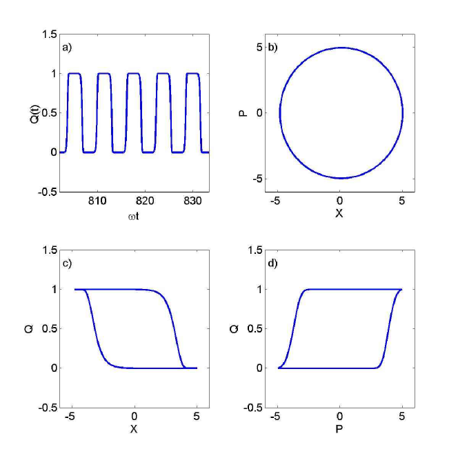
Refer to caption
Figure 7.6: Different representations of the limit cycle solution of the system of differential equations (7.43) that describes the shuttling regime. a) Charge on the dot as a function of time. The charging and discharging times are the shortest time scales. b) Circular trajectory in the mechanical phase space: the motion of the dot is harmonic. c) Projection of the limit cycle in the charge position plane: the trajectory shows charge-position correlation. d) Projection of the limit cycle in the charge momentum plane: the trajectory shows charge-momentum correlation. X𝑋X is the coordinate in units of the tunneling length λ𝜆\lambda, while P𝑃P is the momentum in units of mωλ𝑚𝜔𝜆m\omega\lambda.
Refer to caption
Figure 7.7: Correspondence between the Wigner function representation and the simplified trajectory limit for the shuttling regime. The white ring is the (X,P𝑋𝑃X,P) projection of the limit cycle. The Q=1𝑄1Q=1 and Q=0𝑄0Q=0 portions of the trajectory are visible in the charged and empty dot graphs respectively. The parameters are γ=0.02ω𝛾0.02𝜔\gamma=0.02\omega, d=0.5x0𝑑0.5subscript𝑥0d=0.5x_{0}, Γ=0.05ωΓ0.05𝜔\Gamma=0.05\omega in the first two rows and Γ=0.01Γ0.01\Gamma=0.01 in the last one. The tunneling length is λ=x0𝜆subscript𝑥0\lambda=x_{0} in the first row and λ=2x0𝜆2subscript𝑥0\lambda=2x_{0} in the second and the third.

In the semiclassical description we also have direct access to the current as a function of the time. For example the right lead current reads:

IR(τ)=Q(τ)ΓRe2X(τ)subscript𝐼𝑅𝜏𝑄𝜏subscriptΓ𝑅superscript𝑒2𝑋𝜏I_{R}(\tau)=Q(\tau)\Gamma_{R}e^{2X(\tau)} (7.45)

In figure 7.8 the right current is presented as a function of time for a few mechanical oscillation periods. The current is given by a series of spikes that well represent the single electron released to the right lead after being shuttled by the oscillating dot.
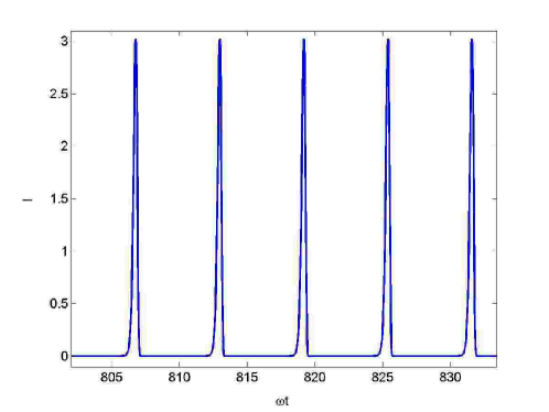
Refer to caption
Figure 7.8: Time resolved shuttling current calculated on the limit cycle solution of the system of differential equations (7.43). The regular spikes well represent the single electron shuttled per cycle in this regime.

The average current is a coarse grained measurement of the time dependent current. Since the current is periodic, if the measurement time is long enough we obtain a stationary current:

Istat=12πττ+2π𝑑τIR(τ)superscript𝐼stat12𝜋superscriptsubscript𝜏𝜏2𝜋differential-dsuperscript𝜏subscript𝐼𝑅superscript𝜏I^{\rm stat}=\frac{1}{2\pi}\int_{\tau}^{\tau+2\pi}\!\!d\tau^{\prime}\,I_{R}(\tau^{\prime}) (7.46)

Since the current is a periodic function of time the average over one period is equal to the average over an infinite time. The numerical integration of the function plotted in figure 7.8 gives

Istat=0.15916superscript𝐼stat0.15916I^{\rm stat}=0.15916 (7.47)

which is with impressive accuracy the “magic value” of 1/2π12𝜋1/2\pi (i.e. one electron transferred per oscillation period).

Also for the TDQS we tried a semiclassical analysis of the shuttling regime. For the derivation of the semiclassical equations we start again from the Hamiltonian (2.9) but we consider x𝑥x and p𝑝p as classical variables. The GME equation for the reduced density matrix σ𝜎\sigma is derived by keeping x𝑥x as a parameter (p𝑝p does not enter explicitly the formulation of the GME). Since the oscillator is treated classically also the elements of the density matrix σijsubscript𝜎𝑖𝑗\sigma_{ij} are now real numbers and the trace sum rule can be used to reduce the effective number of equation for the electrical dynamics141414Also in this case the elements σ0isubscript𝜎0𝑖\sigma_{0i} and σi0subscript𝜎𝑖0\sigma_{i0} with i=L,C,R𝑖𝐿𝐶𝑅i=L,C,R vanish identically reducing the effective number of equations from 16 to 10. from 10 to 9. The GME in matrix notation reads:

σ˙=i[Hsys,σ]+Ξ[σ]˙𝜎𝑖Planck-constant-over-2-pisubscript𝐻𝑠𝑦𝑠𝜎Ξdelimited-[]𝜎\dot{\sigma}=-\frac{i}{\hbar}[H_{sys},\sigma]+\Xi[\sigma] (7.48)

where

Hsys=12mω2x2+p22m+(ΔV2tL(x)0tL(x)ΔV2x0xtR(x)0tR(x)ΔV2)subscript𝐻sys12𝑚superscript𝜔2superscript𝑥2superscript𝑝22𝑚matrixΔ𝑉2subscript𝑡𝐿𝑥0subscript𝑡𝐿𝑥Δ𝑉2subscript𝑥0𝑥subscript𝑡𝑅𝑥0subscript𝑡𝑅𝑥Δ𝑉2H_{\rm sys}=\frac{1}{2}m\omega^{2}x^{2}+\frac{p^{2}}{2m}+\begin{pmatrix}\frac{\Delta V}{2}&t_{L}(x)&0\\ t_{L}(x)&-\frac{\Delta V}{2x_{0}}x&t_{R}(x)\\ 0&t_{R}(x)&-\frac{\Delta V}{2}\end{pmatrix} (7.49)

and the driving Liouvillean ΞΞ\Xi has the form

Ξ[σ]=Γ(1σLLσCCσRR0σLR/200σCR/2σRL/2σRC/2σRR)Ξdelimited-[]𝜎Γmatrix1subscript𝜎𝐿𝐿subscript𝜎𝐶𝐶subscript𝜎𝑅𝑅0subscript𝜎𝐿𝑅200subscript𝜎𝐶𝑅2subscript𝜎𝑅𝐿2subscript𝜎𝑅𝐶2subscript𝜎𝑅𝑅\Xi[\sigma]=\Gamma\begin{pmatrix}1-\sigma_{LL}-\sigma_{CC}-\sigma_{RR}&0&-\sigma_{LR}/2\\ 0&0&-\sigma_{CR}/2\\ -\sigma_{RL}/2&-\sigma_{RC}/2&-\sigma_{RR}\end{pmatrix} (7.50)

where we have taken ΓL=ΓR=ΓsubscriptΓ𝐿subscriptΓ𝑅Γ\Gamma_{L}=\Gamma_{R}=\Gamma. As equation of motion for the mechanical variables x𝑥x and p𝑝p we take the Hamilton equations derived from the effective Hamiltonian

Hsys=Trel[σHsys]delimited-⟨⟩subscript𝐻syssubscriptTreldelimited-[]𝜎subscript𝐻sys\langle H_{\rm sys}\rangle={\rm Tr}_{\rm el}[\sigma H_{\rm sys}] (7.51)

where TrelsubscriptTrel{\rm Tr}_{\rm el} is the trace on the electronic states, combined with a phenomenological friction:

x˙=Hsysp=pmp˙=Hsysxγp=mω2x+ΔV2x0σCCγp+tLλ(σCL+σLC)tRλ(σCR+σRC)˙𝑥delimited-⟨⟩subscript𝐻sys𝑝𝑝𝑚˙𝑝delimited-⟨⟩subscript𝐻sys𝑥𝛾𝑝𝑚superscript𝜔2𝑥Δ𝑉2subscript𝑥0subscript𝜎𝐶𝐶𝛾𝑝subscript𝑡𝐿𝜆subscript𝜎𝐶𝐿subscript𝜎𝐿𝐶subscript𝑡𝑅𝜆subscript𝜎𝐶𝑅subscript𝜎𝑅𝐶\begin{split}\dot{x}=&\frac{\partial\langle H_{\rm sys}\rangle}{\partial p}=\frac{p}{m}\\ \dot{p}=&-\frac{\partial\langle H_{\rm sys}\rangle}{\partial x}-\gamma p=-m\omega^{2}x+\frac{\Delta V}{2x_{0}}\sigma_{CC}-\gamma p\\ &+\frac{t_{L}}{\lambda}(\sigma_{CL}+\sigma_{LC})-\frac{t_{R}}{\lambda}(\sigma_{CR}+\sigma_{RC})\end{split} (7.52)

The phase space has now 11 dimensions (9 electrical and 2 mechanical) but the principle is the same as in the SDQS. Also in this case the solution of the system of differential equations (7.48) and (7.52) exhibits for parameters that correspond to the shuttling regime a stable limit cycle solution. In figure 7.9 we compare the Wigner distribution function for the central dot with the projection on the (x,p)𝑥𝑝(x,p) plane of the limit cycle trajectory of the semiclassical approximation. The probability to find the electron on the central dot σCCsubscript𝜎𝐶𝐶\sigma_{CC} is not in general oscillating between 0 and 1. The red dots in the figure indicate the position of the maximum occupation. In the TDQS the half moon characteristic of the shuttling regime rotates in the phase space [10], close to the first two electromechanical resonances, as a function of the device bias. The correspondence between the darker areas of the Wigner function and the red dots in figure 7.9 shows that also this property is captured by the semiclassical approximation.
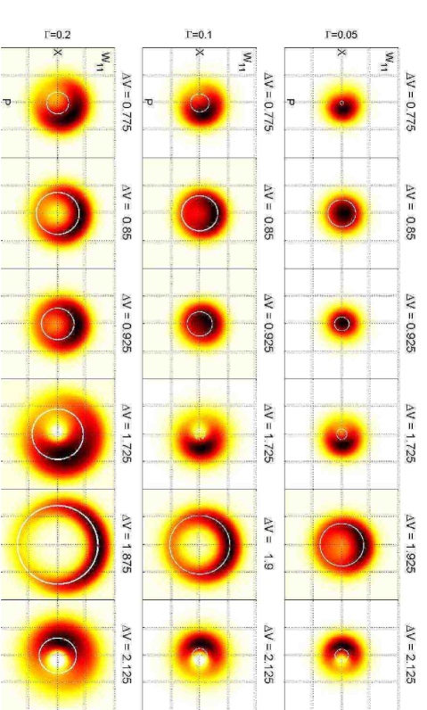
Refer to caption
Figure 7.9: Comparison between the semiclassical approximation and the full description for TDQS. The figure shows the central dot Wigner function and the respective limit cycle. The dark dot on the trajectory is in correspondence with the maximum of the semiclassical occupation σCCsubscript𝜎𝐶𝐶\sigma_{CC}. Also the phase space rotation is captured by the simplified model. The matching is best in the shuttling regime. See figure 5.4 for the details on the parameters.

7.3 Coexistence: a dichotomous process

The slowest dynamics in the coexistence regime is represented by the switching process between the shuttling and the tunneling regime. The amplitude of the dot oscillations is the relevant variable that is recording this slow dynamics. We analyze this particular operating regime of the SDQS in three steps. We first assume the slow switching mode between two different current channels and explore the consequences of this hypothesis in terms of current and current noise. We then derive the effective bistable potential for the amplitude associated with the slowest dynamics of the shuttle device in the coexistence regime. Finally we apply Kramers’ theory for escape rates to this effective potential and calculate the switching rates between the two amplitude equilibrium states corresponding to the local minima of the potential. We conclude the section comparing the (semi)analytical results of the simplified model with the numerical calculations corresponding to the full description.
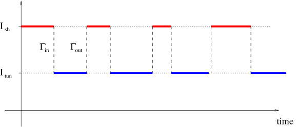
Refer to caption
Figure 7.10: Schematic representation of the time evolution of the current in the dichotomous process between current modes. The scheme refers in particular to the SDQS coexistence regime where the currents involved are the shuttling (Ishsubscript𝐼shI_{\rm sh}) and the tunneling (Itunsubscript𝐼tunI_{\rm tun}) currents and the names of switching rates ΓinsubscriptΓin\Gamma_{\rm in} and ΓoutsubscriptΓout\Gamma_{\rm out} indicate the behaviour of the dot oscillation amplitude (the relevant variable in the model) during the transition.

7.3.1 Dichotomous process between current modes

Let us consider a bistable system with two different modes ++ and - and two different currents I+subscript𝐼I_{+} and Isubscript𝐼I_{-}, respectively, associated with the modes. The system can switch between mode ++ and - randomly, but with definite rates: namely α𝛼\alpha for the process ++\to- and β𝛽\beta for the opposite +-\to+. We collect this information in the master equation:

𝐏˙=ddt(P+P)=(αβαβ)(P+P)=𝐋𝐏˙𝐏𝑑𝑑𝑡matrixsubscript𝑃subscript𝑃matrix𝛼𝛽𝛼𝛽matrixsubscript𝑃subscript𝑃𝐋𝐏\dot{\mathbf{P}}=\frac{d}{dt}\begin{pmatrix}P_{+}\\ P_{-}\\ \end{pmatrix}=\begin{pmatrix}-\alpha&\phantom{-}\beta\\ \phantom{-}\alpha&-\beta\\ \end{pmatrix}\begin{pmatrix}P_{+}\\ P_{-}\\ \end{pmatrix}=\mathbf{LP} (7.53)

where P+subscript𝑃P_{+} and Psubscript𝑃P_{-} are the probabilities to find the system in the mode “++” and “-” respectively.

The matrix notation suggests to read the equation (7.53) at a more general level and embed its classical rate dynamics into a quantum formalism.

Instead of the modes ++ and - we consider the state vectors |+ket|+\rangle and |ket|-\rangle: they define the Hilbert space of the quantum system. Density operators defined on this Hilbert space represent the state of the system. Since we are only interested in classical states we assume that the density matrix σ𝜎\sigma is always diagonal in the |+ket|+\rangle, |ket|-\rangle basis. In terms of the probabilities P𝑃P the density matrix reads obviously:

σ=(σ++σ+σ+σ)=(P+00P)𝜎matrixsubscript𝜎absentsubscript𝜎absentsubscript𝜎absentsubscript𝜎absentmatrixsubscript𝑃00subscript𝑃\sigma=\begin{pmatrix}\sigma_{++}&\sigma_{+-}\\ \sigma_{-+}&\sigma_{--}\end{pmatrix}=\begin{pmatrix}P_{+}&0\\ 0&P_{-}\end{pmatrix} (7.54)

Since each of the two states is associated to a well defined current, also the current operator is diagonal in the +,+,- basis:

I=(I+00I)𝐼matrixsubscript𝐼00subscript𝐼I=\begin{pmatrix}I_{+}&0\\ 0&I_{-}\end{pmatrix} (7.55)

The average current is the trace of the current operator multiplied by the density matrix, namely:

I(t)=Tr[σ(t)I]=P+(t)I++P(t)Idelimited-⟨⟩𝐼𝑡Trdelimited-[]𝜎𝑡𝐼subscript𝑃𝑡subscript𝐼subscript𝑃𝑡subscript𝐼\langle I(t)\rangle={\rm Tr}[\sigma(t)I]=P_{+}(t)I_{+}+P_{-}(t)I_{-} (7.56)

and it is in general time dependent since the occupation probabilities evolve in time according to the equation (7.53).

Equation (7.53) is the equation of motion for the density matrix σ𝜎\sigma. In general the Liouville space151515It is the space of the linear operators on the original Hilbert space. for a system with a Hilbert space of dimension N𝑁N has dimension N2superscript𝑁2N^{2}. In this particular case the system is simplified: the space of the diagonal linear operators has again dimension 2. The equation (7.53) is the representation of the equation:

σ˙=[σ]˙𝜎delimited-[]𝜎\dot{\sigma}=\mathcal{L}[\sigma] (7.57)

in the basis:

𝐞1=(1000),𝐞2=(0001)formulae-sequencesubscript𝐞1matrix1000subscript𝐞2matrix0001\mathbf{e}_{1}=\begin{pmatrix}1&0\\ 0&0\end{pmatrix},\quad\mathbf{e}_{2}=\begin{pmatrix}0&0\\ 0&1\end{pmatrix} (7.58)

with the identification:

σ𝐏=(P+P),𝐋=(αβαβ)formulae-sequence𝜎𝐏matrixsubscript𝑃subscript𝑃𝐋matrix𝛼𝛽𝛼𝛽\sigma\to\mathbf{P}=\begin{pmatrix}P_{+}\\ P_{-}\end{pmatrix},\quad\mathcal{L}\to\mathbf{L}=\begin{pmatrix}-\alpha&\phantom{-}\beta\\ \phantom{-}\alpha&-\beta\end{pmatrix} (7.59)

Until now we have used the Schrödinger picture in which the states evolve. For the definition of the current noise we have to introduce the analogue for open irreversible systems of the Heisenberg picture defined for closed reversible system161616For a rigorous treatment of the argument see for example H.-P. Breuer et al. [46].. The equation (7.57) has the formal solution for a time independent Liouvillean:

σ(t)=etσ(0)𝜎𝑡superscript𝑒𝑡𝜎0\sigma(t)=e^{t\mathcal{L}}\sigma(0) (7.60)

The initial condition σ(0)𝜎0\sigma(0) is evolved to the time t𝑡t by the super-operator etsuperscript𝑒𝑡e^{t\mathcal{L}}. The Heisenberg picture for the operators is designed to preserve the average:

I(t)=Tr[ISσ(t)]=Tr[ISetσ(0)]=Tr[etISσ(0)]=Tr[IH(t)σ(0)]delimited-⟨⟩𝐼𝑡Trdelimited-[]subscript𝐼𝑆𝜎𝑡Trdelimited-[]subscript𝐼𝑆superscript𝑒𝑡𝜎0Trdelimited-[]superscript𝑒𝑡superscriptsubscript𝐼𝑆𝜎0Trdelimited-[]subscript𝐼𝐻𝑡𝜎0\langle I(t)\rangle={\rm Tr}[I_{S}\sigma(t)]={\rm Tr}[I_{S}e^{t\mathcal{L}}\sigma(0)]={\rm Tr}[e^{t\mathcal{L}^{\dagger}}I_{S}\sigma(0)]={\rm Tr}[I_{H}(t)\sigma(0)] (7.61)

where the (current) operator appears first in the Schrödinger ISsubscript𝐼𝑆I_{S}, and then in the Heisenberg IH(t)subscript𝐼𝐻𝑡I_{H}(t) picture. superscript\mathcal{L}^{\dagger} is the adjoint of the superoperator \mathcal{L}. It is useful to consider the representation of the above equations in the basis (7.58):

I(t)=(𝐈S,𝐏(t))=(𝐈,et𝐋𝐏(0))=(et𝐋𝐈,𝐏(0))=(𝐈H(t),𝐏(0))delimited-⟨⟩𝐼𝑡subscript𝐈𝑆𝐏𝑡𝐈superscript𝑒𝑡𝐋𝐏0superscript𝑒𝑡superscript𝐋𝐈𝐏0subscript𝐈𝐻𝑡𝐏0\langle I(t)\rangle=(\mathbf{I}_{S},\mathbf{P}(t))=(\mathbf{I},e^{t\mathbf{L}}\mathbf{P}(0))=(e^{t\mathbf{L}^{\dagger}}\mathbf{I},\mathbf{P}(0))=(\mathbf{I}_{H}(t),\mathbf{P}(0)) (7.62)

where 𝐈S=[I+,I]Tsubscript𝐈𝑆superscriptsubscript𝐼subscript𝐼𝑇\mathbf{I}_{S}=[I_{+},I_{-}]^{T} is the vector representation of the current operator in Schrödinger picture. It is also not difficult to realize that the trace of the product of two operators is equivalent to the scalar product in the vector representation. The current-noise is the spectral density of the average current fluctuations:

S(ω)=limt+𝑑τ[I(t+τ)I(t)I(t+τ)I(t)]eiωτ𝑆𝜔subscript𝑡superscriptsubscriptdifferential-d𝜏delimited-[]delimited-⟨⟩𝐼𝑡𝜏𝐼𝑡delimited-⟨⟩𝐼𝑡𝜏delimited-⟨⟩𝐼𝑡superscript𝑒𝑖𝜔𝜏S(\omega)=\lim_{t\to\infty}\int_{-\infty}^{+\infty}\!\!\!d\tau[\langle I(t+\tau)I(t)\rangle-\langle I(t+\tau)\rangle\langle I(t)\rangle]\,e^{i\omega\tau} (7.63)

In terms of the current operators in the Heisenberg picture, the noise reads:

S(ω)=limt+dτ{Tr[IH(t+τ)IH(t)σ(0)]Tr[IH(t+τ)σ(0)]Tr[IH(t)σ(0)]}eiωτ𝑆𝜔subscript𝑡superscriptsubscript𝑑𝜏Trdelimited-[]subscript𝐼𝐻𝑡𝜏subscript𝐼𝐻𝑡𝜎0Trdelimited-[]subscript𝐼𝐻𝑡𝜏𝜎0Trdelimited-[]subscript𝐼𝐻𝑡𝜎0superscript𝑒𝑖𝜔𝜏\begin{split}S(\omega)=\lim_{t\to\infty}\int_{-\infty}^{+\infty}\!\!\!d\tau\{&{\rm Tr}[I_{H}(t+\tau)I_{H}(t)\sigma(0)]\\ -&{\rm Tr}[I_{H}(t+\tau)\sigma(0)]{\rm Tr}[I_{H}(t)\sigma(0)]\}e^{i\omega\tau}\end{split} (7.64)

The system tends for large times to the stationary state:

P+stat=βα+βPstat=αα+βsuperscriptsubscript𝑃stat𝛽𝛼𝛽superscriptsubscript𝑃stat𝛼𝛼𝛽\begin{split}P_{+}^{\rm stat}&=\frac{\beta}{\alpha+\beta}\\ P_{-}^{\rm stat}&=\frac{\alpha}{\alpha+\beta}\end{split} (7.65)

as can be verified by substitution in (7.53). The corresponding stationary current reads:

Istat=limtI(t)=I+β+Iαα+βsuperscript𝐼statsubscript𝑡delimited-⟨⟩𝐼𝑡subscript𝐼𝛽subscript𝐼𝛼𝛼𝛽I^{\rm stat}=\lim_{t\to\infty}\langle I(t)\rangle=\frac{I_{+}\beta+I_{-}\alpha}{\alpha+\beta} (7.66)

We are interested in the zero frequency noise spectrum ω0𝜔0\omega\to 0. We split the integral into two parts: over negative and positive τ𝜏\tau respectively. Using the symmetry under time reversal ττ𝜏𝜏\tau\to-\tau of the integrand we obtain:

S(0)=limω0limt2[0𝑑τ(Tr[IH(t+τ)IH(t)σ(0)]Istat2)ei(ω+iε)τ]𝑆0subscript𝜔0subscript𝑡2superscriptsubscript0differential-d𝜏Trdelimited-[]subscript𝐼𝐻𝑡𝜏subscript𝐼𝐻𝑡𝜎0superscriptsuperscript𝐼stat2superscript𝑒𝑖𝜔𝑖𝜀𝜏S(0)=\lim_{\omega\to 0}\lim_{t\to\infty}2\Re\left[\int_{0}^{\infty}\!\!\!d\tau\left({\rm Tr}[I_{H}(t+\tau)I_{H}(t)\sigma(0)]-{I^{\rm stat}}^{2}\right)e^{i(\omega+i\varepsilon)\tau}\right] (7.67)

where we have also added to the frequency the small imaginary convergence factor iε𝑖𝜀i\varepsilon. We now use the quantum regression theorem to rewrite the current-current correlator and perform the limit in t𝑡t:

S(0)=limω02[0𝑑τ(Tr[IeτIσstat]Istat2)ei(ω+iε)τ]𝑆0subscript𝜔02superscriptsubscript0differential-d𝜏Trdelimited-[]𝐼superscript𝑒𝜏𝐼superscript𝜎statsuperscriptsuperscript𝐼stat2superscript𝑒𝑖𝜔𝑖𝜀𝜏S(0)=\lim_{\omega\to 0}2\Re\left[\int_{0}^{\infty}\!\!\!d\tau\left({\rm Tr}[Ie^{\tau\mathcal{L}}I\sigma^{\rm stat}]-{I^{\rm stat}}^{2}\right)e^{i(\omega+i\varepsilon)\tau}\right] (7.68)

We then integrate in τ𝜏\tau and obtain:

S(0)=limω02[Tr[I(+iω)1Iσstat]Istat2iω]𝑆0subscript𝜔02Trdelimited-[]𝐼superscript𝑖𝜔1𝐼superscript𝜎statsuperscriptsuperscript𝐼stat2𝑖𝜔S(0)=\lim_{\omega\to 0}2\Re\left[{\rm Tr}[I(\mathcal{L}+i\omega)^{-1}I\sigma^{\rm stat}]-\frac{{I^{\rm stat}}^{2}}{i\omega}\right] (7.69)

In the limit ω0𝜔0\omega\to 0 the resolvent (+iω)1superscript𝑖𝜔1(\mathcal{L}+i\omega)^{-1} is singular since \mathcal{L} has a non-trivial null space. To handle this singularity we introduce the super-operator projectors:

𝒫[]=σstatTr[],𝒬=1𝒫formulae-sequence𝒫delimited-[]superscript𝜎statTrdelimited-[]𝒬1𝒫\mathcal{P}[\bullet]=\sigma^{\rm stat}{\rm Tr}[\bullet],\quad\mathcal{Q}=1-\mathcal{P} (7.70)

We already encountered these projectors in section 5.3.2 where we discussed their properties (5.34). In terms of these projectors the resolvent can be rewritten:

(+iω)1=𝒬(+iω)1𝒬+𝒫iωsuperscript𝑖𝜔1𝒬superscript𝑖𝜔1𝒬𝒫𝑖𝜔(\mathcal{L}+i\omega)^{-1}=\mathcal{Q}(\mathcal{L}+i\omega)^{-1}\mathcal{Q}+\frac{\mathcal{P}}{i\omega} (7.71)

The term 𝒬(+iω)1𝒬𝒬superscript𝑖𝜔1𝒬\mathcal{Q}(\mathcal{L}+i\omega)^{-1}\mathcal{Q} is well-behaved in the limit ω0𝜔0\omega\to 0 since the 𝒬𝒬\mathcal{Q} projectors are confining the inverse of the Liouvillean on the subspace orthogonal to the null space. The term 𝒫iω𝒫𝑖𝜔\frac{\mathcal{P}}{i\omega} is still singular. However, using the definition (7.70) we can calculate:

Tr[I𝒫iωIσstat]=Tr[IIstatiωσstat]=Istat2iωTrdelimited-[]𝐼𝒫𝑖𝜔𝐼superscript𝜎statTrdelimited-[]𝐼superscript𝐼stat𝑖𝜔superscript𝜎statsuperscriptsuperscript𝐼stat2𝑖𝜔{\rm Tr}\left[I\frac{\mathcal{P}}{i\omega}I\sigma^{\rm stat}\right]={\rm Tr}\left[I\frac{I^{\rm stat}}{i\omega}\sigma^{\rm stat}\right]=\frac{{I^{\rm stat}}^{2}}{i\omega} (7.72)

and notice that the two diverging contribution in the current noise exactly cancel. The zero frequency current noise reads:

S(0)=2Tr(I𝒬1𝒬Iσstat)𝑆02Tr𝐼𝒬superscript1𝒬𝐼superscript𝜎statS(0)=-2{\rm Tr}(I\mathcal{QL}^{-1}\mathcal{Q}I\sigma^{\rm stat}) (7.73)

For the evaluation of the current noise S(0)𝑆0S(0) we introduce the auxiliary quantity ΣΣ\Sigma

Σ=𝒬1𝒬IσstatΣ𝒬superscript1𝒬𝐼superscript𝜎stat\Sigma=\mathcal{QL}^{-1}\mathcal{Q}I\sigma^{\rm stat} (7.74)

so that

S(0)=2Tr(IΣ)=2(𝐈,𝚺)𝑆02Tr𝐼Σ2𝐈𝚺S(0)=-2{\rm Tr}(I\Sigma)=-2(\mathbf{I},\mathbf{\Sigma}) (7.75)

where we have used in the last equality the vector notation characteristic of the example at hand. The quantity ΣΣ\Sigma satisfies the equation:

Σ=𝒬Iσstat=(IIstat)σstatΣ𝒬𝐼superscript𝜎stat𝐼superscript𝐼statsuperscript𝜎stat\mathcal{L}\Sigma=\mathcal{Q}I\sigma^{\rm stat}=(I-I^{\rm stat})\sigma^{\rm stat} (7.76)

that in vector notation reads

(αβαβ)(Σ+Σ)=(I+I)α+β(αβ)matrix𝛼𝛽𝛼𝛽matrixsubscriptΣsubscriptΣsubscript𝐼subscript𝐼𝛼𝛽matrix𝛼𝛽\begin{pmatrix}-\alpha&\beta\\ \alpha&-\beta\end{pmatrix}\begin{pmatrix}\Sigma_{+}\\ \Sigma_{-}\end{pmatrix}=\frac{(I_{+}-I_{-})}{\alpha+\beta}\begin{pmatrix}\alpha\\ -\beta\end{pmatrix} (7.77)

The components of the vector 𝚺𝚺\mathbf{\Sigma} also satisfy the independent relation Σ++Σ=0subscriptΣsubscriptΣ0\Sigma_{+}+\Sigma_{-}=0. We solve then for 𝚺𝚺\mathbf{\Sigma} and we are able to give an analytical expression for the noise of the dichotomous process:

S(0)=2αβ(α+β)3ΔI2𝑆02𝛼𝛽superscript𝛼𝛽3Δsuperscript𝐼2S(0)=2\frac{\alpha\beta}{(\alpha+\beta)^{3}}\Delta I^{2} (7.78)

where ΔI=I+IΔ𝐼subscript𝐼subscript𝐼\Delta I=I_{+}-I_{-}. Summarizing, we give the expression for the stationary current and Fano factor for a dichotomous process between two current modes with currents I+subscript𝐼I_{+} and Isubscript𝐼I_{-} and switching rates α𝛼\alpha and β𝛽\beta:

Istat=I+β+Iαα+βF=S(0)Istat=2αβ(α+β)2(I+I)2I+β+Iαsuperscript𝐼statsubscript𝐼𝛽subscript𝐼𝛼𝛼𝛽𝐹𝑆0superscript𝐼stat2𝛼𝛽superscript𝛼𝛽2superscriptsubscript𝐼subscript𝐼2subscript𝐼𝛽subscript𝐼𝛼\begin{split}&I^{\rm stat}=\frac{I_{+}\beta+I_{-}\alpha}{\alpha+\beta}\\ &F=\frac{S(0)}{I^{\rm stat}}=2\frac{\alpha\beta}{(\alpha+\beta)^{2}}\frac{(I_{+}-I_{-})^{2}}{I_{+}\beta+I_{-}\alpha}\end{split} (7.79)

The framework of the coexistence simplified model is given by these results. The task is now to recognize in the dynamics of the shuttle device the two modes and above all calculate the switching rates. The answer are in the Kramers’ escape rates for a bistable effective potential.

7.3.2 Effective potential

The stationary total Wigner function for the SDQS evolves as a function of the mechanical damping from a fuzzy dot close to the origin of the phase space (tunneling regime) to a growing ring-shape in the small damping (shuttling) regime. At intermediate damping rates the shuttling ring and the tunneling fuzzy dot coexist. Those properties of the Wigner function can be understood in terms of an effective stationary potential in the phase space generated by the non-linear dynamics of the shuttle device. We show in figure 7.11 the three qualitatively different shapes of the potential guessed from the observation of the stationary Wigner functions associated with the three operating regimes. Fedorets et al. [9] started the analytical work for the understanding of the tunneling-shuttling transition171717Very recently they also introduced the spin degree of freedom in the oscillating dot [47]. in terms of an effective radial potential. Taking inspiration from their work we extend the analysis to the slowest dynamics in the device and use quantitatively the idea of the effective potential for the description of the coexistence regime.
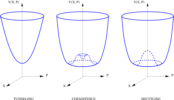
Refer to caption
Figure 7.11: Schematic representation of the effective potentials for the three operating regimes.
Elimination of the fast dynamics

The starting point are the Klein-Kramers equations for the SDQS that we rewrite symmetrized by shifting the coordinates origin to d/2𝑑2d/2:

W00t=[mω2(q+d2)ppmq+γpp+γmω(nB+12)2p2]W00+ΓRe2q/λW11ΓLe2q/λn=0(1)n(2n)!(λ)2n2nW00p2nW11t=[mω2(qd2)ppmq+γpp+γmω(nB+12)2p2]W11+ΓLe2q/λW00ΓRe2q/λn=0(1)n(2n)!(λ)2n2nW11p2nsubscript𝑊00𝑡delimited-[]𝑚superscript𝜔2𝑞𝑑2𝑝𝑝𝑚𝑞𝛾𝑝𝑝𝛾𝑚Planck-constant-over-2-pi𝜔subscript𝑛𝐵12superscript2superscript𝑝2subscript𝑊00subscriptΓ𝑅superscript𝑒2𝑞𝜆subscript𝑊11subscriptΓ𝐿superscript𝑒2𝑞𝜆superscriptsubscript𝑛0superscript1𝑛2𝑛superscriptPlanck-constant-over-2-pi𝜆2𝑛superscript2𝑛subscript𝑊00superscript𝑝2𝑛subscript𝑊11𝑡delimited-[]𝑚superscript𝜔2𝑞𝑑2𝑝𝑝𝑚𝑞𝛾𝑝𝑝𝛾𝑚Planck-constant-over-2-pi𝜔subscript𝑛𝐵12superscript2superscript𝑝2subscript𝑊11subscriptΓ𝐿superscript𝑒2𝑞𝜆subscript𝑊00subscriptΓ𝑅superscript𝑒2𝑞𝜆superscriptsubscript𝑛0superscript1𝑛2𝑛superscriptPlanck-constant-over-2-pi𝜆2𝑛superscript2𝑛subscript𝑊11superscript𝑝2𝑛\begin{split}\frac{\partial W_{00}}{\partial t}=&\left[m\omega^{2}\left(q+\frac{d}{2}\right)\frac{\partial}{\partial p}-\frac{p}{m}\frac{\partial}{\partial q}+\gamma\frac{\partial}{\partial p}p+\gamma m\hbar\omega\left(n_{B}+\frac{1}{2}\right)\frac{\partial^{2}}{\partial p^{2}}\right]W_{00}\\ &+\Gamma_{R}e^{2q/\lambda}W_{11}-\Gamma_{L}e^{-2q/\lambda}\sum_{n=0}^{\infty}\frac{(-1)^{n}}{(2n)!}\left(\frac{\hbar}{\lambda}\right)^{2n}\frac{\partial^{2n}W_{00}}{\partial p^{2n}}\\ \frac{\partial W_{11}}{\partial t}=&\left[m\omega^{2}\left(q-\frac{d}{2}\right)\frac{\partial}{\partial p}-\frac{p}{m}\frac{\partial}{\partial q}+\gamma\frac{\partial}{\partial p}p+\gamma m\hbar\omega\left(n_{B}+\frac{1}{2}\right)\frac{\partial^{2}}{\partial p^{2}}\right]W_{11}\\ &+\Gamma_{L}e^{-2q/\lambda}W_{00}-\Gamma_{R}e^{2q/\lambda}\sum_{n=0}^{\infty}\frac{(-1)^{n}}{(2n)!}\left(\frac{\hbar}{\lambda}\right)^{2n}\frac{\partial^{2n}W_{11}}{\partial p^{2n}}\end{split} (7.80)

One by one we will now get rid of the variables that due to their fast dynamics are not relevant for the description of the coexistence regime. In equations (7.80) we describe the electrical state of the dot as empty or charged. We shift to the description in terms of state ++ and state - with the definition:

W+=W00+W11,W=W00W11formulae-sequencesubscript𝑊subscript𝑊00subscript𝑊11subscript𝑊subscript𝑊00subscript𝑊11W_{+}=W_{00}+W_{11},\quad W_{-}=W_{00}-W_{11} (7.81)

In terms of these new Wigner functions the Klein-Kramers equations read:

tW+={Hosc,W+}P+1W++2WtW={Hosc,W}P+(1+Γ+)W+(2+Γ)W+subscript𝑡subscript𝑊subscriptsubscript𝐻oscsubscript𝑊𝑃subscript1subscript𝑊subscript2subscript𝑊subscript𝑡subscript𝑊subscriptsubscript𝐻oscsubscript𝑊𝑃subscript1subscriptΓsubscript𝑊subscript2subscriptΓsubscript𝑊\begin{split}\partial_{t}W_{+}&=\{H_{\rm osc},W_{+}\}_{P}+\mathcal{L}_{1}W_{+}+\mathcal{L}_{2}W_{-}\\ \partial_{t}W_{-}&=\{H_{\rm osc},W_{-}\}_{P}+(\mathcal{L}_{1}+\Gamma_{+})W_{-}+(\mathcal{L}_{2}+\Gamma_{-})W_{+}\\ \end{split} (7.82)

where

Γ+=ΓRe2q/λ+ΓLe2q/λΓ=ΓRe2q/λΓLe2q/λ1=γpp+γmω(nB+12)p2Γ+2n=112n!(iλ)2np2n2=e2p+Γ2n=112n!(iλ)2np2nsubscriptΓsubscriptΓ𝑅superscript𝑒2𝑞𝜆subscriptΓ𝐿superscript𝑒2𝑞𝜆subscriptΓsubscriptΓ𝑅superscript𝑒2𝑞𝜆subscriptΓ𝐿superscript𝑒2𝑞𝜆subscript1𝛾subscript𝑝𝑝𝛾𝑚Planck-constant-over-2-pi𝜔subscript𝑛𝐵12subscriptsuperscript2𝑝subscriptΓ2superscriptsubscript𝑛112𝑛superscriptPlanck-constant-over-2-pi𝑖𝜆2𝑛subscriptsuperscript2𝑛𝑝subscript2𝑒2𝑝subscriptΓ2superscriptsubscript𝑛112𝑛superscriptPlanck-constant-over-2-pi𝑖𝜆2𝑛superscriptsubscript𝑝2𝑛\begin{split}\Gamma_{+}&=\Gamma_{R}e^{2q/\lambda}+\Gamma_{L}e^{-2q/\lambda}\\ \Gamma_{-}&=\Gamma_{R}e^{2q/\lambda}-\Gamma_{L}e^{-2q/\lambda}\\ \mathcal{L}_{1}&=\gamma\partial_{p}p+\gamma m\hbar\omega\left(n_{B}+\frac{1}{2}\right)\partial^{2}_{p}-\frac{\Gamma_{+}}{2}\sum_{n=1}^{\infty}\frac{1}{2n!}\left(\frac{\hbar}{i\lambda}\right)^{2n}\partial^{2n}_{p}\\ \mathcal{L}_{2}&=\frac{e\mathcal{E}}{2}\frac{\partial}{\partial p}+\frac{\Gamma_{-}}{2}\sum_{n=1}^{\infty}\frac{1}{2n!}\left(\frac{\hbar}{i\lambda}\right)^{2n}\partial_{p}^{2n}\end{split} (7.83)

The symbol {,}Psubscript𝑃\{\bullet,\bullet\}_{P} represents the Poisson brackets and we have introduced for the partial derivatives the short notation xxsubscript𝑥𝑥\partial_{x}\equiv\frac{\partial}{\partial x}. It is useful for the calculation of the effective potential to treat position and momentum on equal footing. For this reason we introduce the adimensional variables:

X=qλ,P=pmλω,τ=tωformulae-sequence𝑋𝑞𝜆formulae-sequence𝑃𝑝𝑚𝜆𝜔𝜏𝑡𝜔X=\frac{q}{\lambda},\quad P=\frac{p}{m\lambda\omega},\quad\tau=t\omega (7.84)

The general structure of the equations (7.82) remains unchanged but the Liouvilleans and the ΓΓ\Gamma functions take the form:

Γ+=ΓRωe2X+ΓLωe2XΓ=ΓRωe2XΓLωe2X1=γωPP+γω(x0λ)2(nB+12)P2Γ+2n=1(1)n2n!(x0λ)4nP2n2=d2λP+Γ2n=1(1)n2n!(x0λ)4nP2nsubscriptΓsubscriptΓ𝑅𝜔superscript𝑒2𝑋subscriptΓ𝐿𝜔superscript𝑒2𝑋subscriptΓsubscriptΓ𝑅𝜔superscript𝑒2𝑋subscriptΓ𝐿𝜔superscript𝑒2𝑋subscript1𝛾𝜔subscript𝑃𝑃𝛾𝜔superscriptsubscript𝑥0𝜆2subscript𝑛𝐵12subscriptsuperscript2𝑃subscriptΓ2superscriptsubscript𝑛1superscript1𝑛2𝑛superscriptsubscript𝑥0𝜆4𝑛subscriptsuperscript2𝑛𝑃subscript2𝑑2𝜆subscript𝑃subscriptΓ2superscriptsubscript𝑛1superscript1𝑛2𝑛superscriptsubscript𝑥0𝜆4𝑛superscriptsubscript𝑃2𝑛\begin{split}\Gamma_{+}&=\frac{\Gamma_{R}}{\omega}e^{2X}+\frac{\Gamma_{L}}{\omega}e^{-2X}\\ \Gamma_{-}&=\frac{\Gamma_{R}}{\omega}e^{2X}-\frac{\Gamma_{L}}{\omega}e^{-2X}\\ \mathcal{L}_{1}&=\frac{\gamma}{\omega}\partial_{P}P+\frac{\gamma}{\omega}\left(\frac{x_{0}}{\lambda}\right)^{2}\left(n_{B}+\frac{1}{2}\right)\partial^{2}_{P}-\frac{\Gamma_{+}}{2}\sum_{n=1}^{\infty}\frac{(-1)^{n}}{2n!}\left(\frac{x_{0}}{\lambda}\right)^{4n}\partial^{2n}_{P}\\ \mathcal{L}_{2}&=\frac{d}{2\lambda}\partial_{P}+\frac{\Gamma_{-}}{2}\sum_{n=1}^{\infty}\frac{(-1)^{n}}{2n!}\left(\frac{x_{0}}{\lambda}\right)^{4n}\partial_{P}^{2n}\end{split} (7.85)

Since in the following we will assume the “classical” limit of a tunneling length much larger than the zero point uncertainty in the position, only the first term of the sums that appears in the definition of 1subscript1\mathcal{L}_{1} and 2subscript2\mathcal{L}_{2} will be kept. Following Fedorets et al. [9] we also introduce polar coordinates:

X=Asinϕ,P=Acosϕformulae-sequence𝑋𝐴italic-ϕ𝑃𝐴italic-ϕX=A\sin\phi,\quad P=A\cos\phi (7.86)

The equations (7.82) are transformed into:

τW+=(ϕ+1)W++2WτW=(ϕ+1Γ+)W+(2+Γ)W+subscript𝜏subscript𝑊subscriptitalic-ϕsubscript1subscript𝑊subscript2subscript𝑊subscript𝜏subscript𝑊subscriptitalic-ϕsubscript1subscriptΓsubscript𝑊subscript2subscriptΓsubscript𝑊\begin{split}\partial_{\tau}W_{+}&=(-\partial_{\phi}+\mathcal{L}_{1})W_{+}+\mathcal{L}_{2}W_{-}\\ \partial_{\tau}W_{-}&=(-\partial_{\phi}+\mathcal{L}_{1}-\Gamma_{+})W_{-}+(\mathcal{L}_{2}+\Gamma_{-})W_{+}\\ \end{split} (7.87)

It is interesting to note that the Poisson brackets for the harmonic oscillator reduce in the polar coordinates to ϕsubscriptitalic-ϕ-\partial_{\phi} since there is no amplitude dynamics in the phase space. The ΓΓ\Gamma functions now read:

Γ+=ΓRωe2Asinϕ+ΓLωe2AsinϕΓ=ΓRωe2AsinϕΓLωe2AsinϕsubscriptΓsubscriptΓ𝑅𝜔superscript𝑒2𝐴italic-ϕsubscriptΓ𝐿𝜔superscript𝑒2𝐴italic-ϕsubscriptΓsubscriptΓ𝑅𝜔superscript𝑒2𝐴italic-ϕsubscriptΓ𝐿𝜔superscript𝑒2𝐴italic-ϕ\begin{split}\Gamma_{+}&=\frac{\Gamma_{R}}{\omega}e^{2A\sin\phi}+\frac{\Gamma_{L}}{\omega}e^{-2A\sin\phi}\\ \Gamma_{-}&=\frac{\Gamma_{R}}{\omega}e^{2A\sin\phi}-\frac{\Gamma_{L}}{\omega}e^{-2A\sin\phi}\end{split} (7.88)

For the transformation of the Liouvilleans 1,2subscript12\mathcal{L}_{1,2} we used the polar coordinate representation of the following differential operators:

P=sinϕAϕ+cosϕA=1AcosϕAA1AϕsinϕP2=2A2cosϕsinϕϕ+sin2ϕAA+sin2ϕA2ϕ22AsinϕcosϕAϕ2+cos2ϕA2=1Acos2ϕA2A2AAϕ2sinϕcosϕ+1A2ϕ2sin2ϕ1AAsin2ϕ2A2ϕcosϕsinϕPP=1Acos2ϕAA2ϕsinϕcosϕ=1sinϕcosϕϕ+cos2ϕAAsubscript𝑃italic-ϕ𝐴subscriptitalic-ϕitalic-ϕsubscript𝐴1𝐴italic-ϕsubscript𝐴𝐴1𝐴subscriptitalic-ϕitalic-ϕsubscriptsuperscript2𝑃2superscript𝐴2italic-ϕitalic-ϕsubscriptitalic-ϕsuperscript2italic-ϕ𝐴subscript𝐴superscript2italic-ϕsuperscript𝐴2subscriptsuperscript2italic-ϕ2𝐴italic-ϕitalic-ϕsubscriptsuperscript2𝐴italic-ϕsuperscript2italic-ϕsubscriptsuperscript2𝐴1𝐴superscript2italic-ϕsubscriptsuperscript2𝐴𝐴2𝐴subscriptsuperscript2𝐴italic-ϕitalic-ϕitalic-ϕ1superscript𝐴2subscriptsuperscript2italic-ϕsuperscript2italic-ϕ1𝐴subscript𝐴superscript2italic-ϕ2superscript𝐴2subscriptitalic-ϕitalic-ϕitalic-ϕsubscript𝑃𝑃1𝐴superscript2italic-ϕsubscript𝐴superscript𝐴2subscriptitalic-ϕitalic-ϕitalic-ϕ1italic-ϕitalic-ϕsubscriptitalic-ϕsuperscript2italic-ϕ𝐴subscript𝐴\begin{split}\partial_{P}=&-\frac{\sin\phi}{A}\partial_{\phi}+\cos\phi\partial_{A}\\ =&\frac{1}{A}\cos\phi\partial_{A}A-\frac{1}{A}\partial_{\phi}\sin\phi\\ \partial^{2}_{P}=&\frac{2}{A^{2}}\cos\phi\sin\phi\partial_{\phi}+\frac{\sin^{2}\phi}{A}\partial_{A}+\frac{\sin^{2}\phi}{A^{2}}\partial^{2}_{\phi}\\ &-\frac{2}{A}\sin\phi\cos\phi\partial^{2}_{A\phi}+\cos^{2}\phi\partial^{2}_{A}\\ =&\frac{1}{A}\cos^{2}\phi\partial^{2}_{A}A-\frac{2}{A}\partial^{2}_{A\phi}\sin\phi\cos\phi+\frac{1}{A^{2}}\partial^{2}_{\phi}\sin^{2}\phi\\ &-\frac{1}{A}\partial_{A}\sin^{2}\phi-\frac{2}{A^{2}}\partial_{\phi}\cos\phi\sin\phi\\ \partial_{P}P=&\frac{1}{A}\cos^{2}\phi\partial_{A}A^{2}-\partial_{\phi}\sin\phi\cos\phi\\ =&1-\sin\phi\cos\phi\partial_{\phi}+\cos^{2}\phi A\partial_{A}\end{split} (7.89)

where Aϕ22Aϕsubscriptsuperscript2𝐴italic-ϕsuperscript2𝐴italic-ϕ\partial^{2}_{A\phi}\equiv\frac{\partial^{2}}{\partial A\partial\phi}. The two different forms (partial differential operator Asubscript𝐴\partial_{A} and/or ϕsubscriptitalic-ϕ\partial_{\phi} to the extreme left or right) that for the moment seem redundant will be very useful in the derivation of the effective potential.

We now start to make approximations on the system of equations (7.87) with the main idea of eliminating the fast irrelevant variables. We know that eventually the density operators σiisubscript𝜎𝑖𝑖\sigma_{ii} that describe the system will reach a stationary state. In absence of the harmonic oscillator the state ++ would be fixed by the trace sum rule and the state - would relax to zero on a time scale fixed by the tunneling rates. We assume that also in the presence of the mechanical degree of freedom the relaxation dynamics of the |ket|-\rangle state is much faster than the one of the |+ket|+\rangle state. We set τWsubscript𝜏subscript𝑊\partial_{\tau}W_{-} to zero in the second equation of (7.87) and formally solve the equation for Wsubscript𝑊W_{-}. We insert the result in the first equation of (7.87) and obtain a closed equation for the (total) Wigner function W+subscript𝑊W_{+}:

τW+=[ϕ+1+2(1G^01)1G^0(2+Γ)+]W+subscript𝜏subscript𝑊delimited-[]subscriptitalic-ϕsubscriptsubscript1subscript2superscript1subscript^𝐺0subscript11subscript^𝐺0subscript2subscriptΓsubscriptsubscript𝑊\begin{split}\partial_{\tau}W_{+}&=[-\partial_{\phi}+\underbrace{\mathcal{L}_{1}+\mathcal{L}_{2}(1-\hat{G}_{0}\mathcal{L}_{1})^{-1}\hat{G}_{0}(\mathcal{L}_{2}+\Gamma_{-})}_{\displaystyle\mathcal{L}_{+}}]W_{+}\\ \end{split} (7.90)

where G^0(ϕ+Γ+)1subscript^𝐺0superscriptsubscriptitalic-ϕsubscriptΓ1\hat{G}_{0}\equiv(\partial_{\phi}+\Gamma_{+})^{-1} and we also define the (super)operator +subscript\mathcal{L}_{+}. At this point the detailed information about the charge state of the oscillating dot is integrated out, but the equation (7.90) still takes the fast phase dynamics into account. Since we are interested only in the amplitude dynamics (the slowest in the coexistence regime) we introduce the projector 𝒫ϕsubscript𝒫italic-ϕ\mathcal{P}_{\phi} that averages over the phase and its orthogonal complement 𝒬ϕ=1𝒫ϕsubscript𝒬italic-ϕ1subscript𝒫italic-ϕ\mathcal{Q}_{\phi}=1-\mathcal{P}_{\phi}:

𝒫ϕ[]=12π02πdϕ\mathcal{P}_{\phi}[\bullet]=\frac{1}{2\pi}\int_{0}^{2\pi}d\phi\bullet (7.91)

Using these two operators we decompose the Wigner distribution function into:

W+=𝒫W++𝒬W+=W¯++W~+subscript𝑊𝒫subscript𝑊𝒬subscript𝑊subscript¯𝑊subscript~𝑊W_{+}=\mathcal{P}W_{+}+\mathcal{Q}W_{+}=\bar{W}_{+}+\tilde{W}_{+} (7.92)

We apply the same projectors also to the equation (7.90) and we obtain the set of coupled partial (integro-181818The operator \mathcal{L} contains the inverse of differential operators.)differential equations:

τW¯+=𝒫ϕ+W¯++𝒫ϕ+W~+τW~+=[ϕ+𝒬ϕ+]W~++𝒬ϕ+W¯+subscript𝜏subscript¯𝑊subscript𝒫italic-ϕsubscriptsubscript¯𝑊subscript𝒫italic-ϕsubscriptsubscript~𝑊subscript𝜏subscript~𝑊delimited-[]subscriptitalic-ϕsubscript𝒬italic-ϕsubscriptsubscript~𝑊subscript𝒬italic-ϕsubscriptsubscript¯𝑊\begin{split}\partial_{\tau}\bar{W}_{+}&=\mathcal{P}_{\phi}\mathcal{L}_{+}\bar{W}_{+}+\mathcal{P}_{\phi}\mathcal{L}_{+}\tilde{W}_{+}\\ \partial_{\tau}\tilde{W}_{+}&=[-\partial_{\phi}+\mathcal{Q}_{\phi}\mathcal{L}_{+}]\tilde{W}_{+}+\mathcal{Q}_{\phi}\mathcal{L}_{+}\bar{W}_{+}\end{split} (7.93)

where we have used the properties:

𝒫ϕϕ=0𝒬ϕϕ=ϕ𝒬ϕ=ϕsubscript𝒫italic-ϕsubscriptitalic-ϕ0subscript𝒬italic-ϕsubscriptitalic-ϕsubscriptitalic-ϕsubscript𝒬italic-ϕsubscriptitalic-ϕ\begin{split}&\mathcal{P}_{\phi}\partial_{\phi}=0\\ &\mathcal{Q}_{\phi}\partial_{\phi}=\partial_{\phi}\mathcal{Q}_{\phi}=\partial_{\phi}\end{split} (7.94)

which is readily demonstrated since all the distributions involved are periodic functions of ϕitalic-ϕ\phi. We now assume that the phase relaxation time that governs the dynamics of the phase-dependent distribution W~+subscript~𝑊\tilde{W}_{+} is much shorter than the amplitude relaxation time of the distribution W+subscript𝑊W_{+} 191919This assumption is based on the observation that the diffusion dynamics that governs the relaxation times is largely facilitated along the transverse direction where no potential barriers (see fig. 7.11) must be overcome. The potential barriers occur instead in the radial direction.. We then set τW~+=0subscript𝜏subscript~𝑊0\partial_{\tau}\tilde{W}_{+}=0 in the second equation of (7.93), solve it for W~+subscript~𝑊\tilde{W}_{+} and insert the result in the first equation. The result is a closed equation for the (quasi)probability distribution function W¯+subscript¯𝑊\bar{W}_{+}:

τW¯+=𝒫ϕ+[1+(1g^0𝒬ϕ+)1g^0𝒬ϕ+]W¯+subscript𝜏subscript¯𝑊subscript𝒫italic-ϕsubscriptdelimited-[]1superscript1subscript^𝑔0subscript𝒬italic-ϕsubscript1subscript^𝑔0subscript𝒬italic-ϕsubscriptsubscript¯𝑊\partial_{\tau}\bar{W}_{+}=\mathcal{P}_{\phi}\mathcal{L}_{+}[1+(1-\hat{g}_{0}\mathcal{Q}_{\phi}\mathcal{L}_{+})^{-1}\hat{g}_{0}\mathcal{Q}_{\phi}\mathcal{L}_{+}]\bar{W}_{+} (7.95)

where g^0(ϕ)1subscript^𝑔0superscriptsubscriptitalic-ϕ1\hat{g}_{0}\equiv(\partial_{\phi})^{-1}. We notice that the operator g^0subscript^𝑔0\hat{g}_{0} is in the equations always following the projector 𝒬ϕsubscript𝒬italic-ϕ\mathcal{Q}_{\phi}. This combination of operators ensures us as an output a periodic function in the variable ϕitalic-ϕ\phi.

Small parameters expansion

We believe that equation (7.95) contains the relevant dynamics of the SDQS in the coexistence regime, but, despite all the approximations already introduced the problem still looks untractable. Again following the already mentioned work by Fedorets et al. [9] we consider the perturbation expansion of (7.95) in the “small parameters”:

dλ,(x0λ)2,γω1much-less-than𝑑𝜆superscriptsubscript𝑥0𝜆2𝛾𝜔1\frac{d}{\lambda},\quad\left(\frac{x_{0}}{\lambda}\right)^{2},\quad\frac{\gamma}{\omega}\ll 1 (7.96)

These three inequalities describe a limit often encountered in this thesis and they correspond respectively to the three physical assumptions:

  1. 1.

    The external electrostatic force is a small perturbation of the harmonic oscillator restoring force in terms of the sensitivity to displacement of the tunneling rates. This ensures a quasi oscillator-independent treatment of the tunneling regime.

  2. 2.

    The tunneling length is big compared to the zero point fluctuations. Since the oscillator dynamics for the shuttling (and then partially also for the coexistence) regime happens on the scale of the tunneling length, this condition ensures a quasi-classical behaviour of the harmonic oscillator.

  3. 3.

    The coupling of the oscillator to the thermal bath is weak and the oscillator dynamics is under-damped.

We want to expand the equation (7.95) up to second order in the three small parameters (7.96). To proceed systematically we first notice that they appear at least to first order in the Liouvilleans 1subscript1\mathcal{L}_{1} and 2subscript2\mathcal{L}_{2} and thus also in the operator +subscript\mathcal{L}_{+}. We can then safely expand (7.95) up to second order in +subscript\mathcal{L}_{+} without missing any desired term:

τW¯+𝒫ϕ+[1+g^0𝒬ϕ+]W¯+subscript𝜏subscript¯𝑊subscript𝒫italic-ϕsubscriptdelimited-[]1subscript^𝑔0subscript𝒬italic-ϕsubscriptsubscript¯𝑊\partial_{\tau}\bar{W}_{+}\approx\mathcal{P}_{\phi}\mathcal{L}_{+}[1+\hat{g}_{0}\mathcal{Q}_{\phi}\mathcal{L}_{+}]\bar{W}_{+} (7.97)

Using the definition of +subscript\mathcal{L}_{+} contained in (7.90) we now expand this last equation up to second order in 1subscript1\mathcal{L}_{1} and 2subscript2\mathcal{L}_{2}:

τW¯+[𝒫ϕ1+𝒫ϕ2G^0Γ+𝒫ϕ2G^01G^0Γ+𝒫ϕ2G^02+𝒫ϕ1g^0𝒬ϕ1+𝒫ϕ2G^0Γg^0𝒬ϕ2G^0Γ+𝒫ϕ1g^0𝒬ϕ2G^0Γ+𝒫ϕ2G^0Γg^0𝒬ϕ1]W¯+subscript𝜏subscript¯𝑊delimited-[]subscript𝒫italic-ϕsubscript1subscript𝒫italic-ϕsubscript2subscript^𝐺0subscriptΓsubscript𝒫italic-ϕsubscript2subscript^𝐺0subscript1subscript^𝐺0subscriptΓsubscript𝒫italic-ϕsubscript2subscript^𝐺0subscript2subscript𝒫italic-ϕsubscript1subscript^𝑔0subscript𝒬italic-ϕsubscript1subscript𝒫italic-ϕsubscript2subscript^𝐺0subscriptΓsubscript^𝑔0subscript𝒬italic-ϕsubscript2subscript^𝐺0subscriptΓsubscript𝒫italic-ϕsubscript1subscript^𝑔0subscript𝒬italic-ϕsubscript2subscript^𝐺0subscriptΓsubscript𝒫italic-ϕsubscript2subscript^𝐺0subscriptΓsubscript^𝑔0subscript𝒬italic-ϕsubscript1subscript¯𝑊\begin{split}\partial_{\tau}\bar{W}_{+}\approx[&\mathcal{P}_{\phi}\mathcal{L}_{1}+\mathcal{P}_{\phi}\mathcal{L}_{2}\hat{G}_{0}\Gamma_{-}\\ +&\mathcal{P}_{\phi}\mathcal{L}_{2}\hat{G}_{0}\mathcal{L}_{1}\hat{G}_{0}\Gamma_{-}+\mathcal{P}_{\phi}\mathcal{L}_{2}\hat{G}_{0}\mathcal{L}_{2}\\ +&\mathcal{P}_{\phi}\mathcal{L}_{1}\hat{g}_{0}\mathcal{Q}_{\phi}\mathcal{L}_{1}+\mathcal{P}_{\phi}\mathcal{L}_{2}\hat{G}_{0}\Gamma_{-}\hat{g}_{0}\mathcal{Q}_{\phi}\mathcal{L}_{2}\hat{G}_{0}\Gamma_{-}\\ +&\mathcal{P}_{\phi}\mathcal{L}_{1}\hat{g}_{0}\mathcal{Q}_{\phi}\mathcal{L}_{2}\hat{G}_{0}\Gamma_{-}+\mathcal{P}_{\phi}\mathcal{L}_{2}\hat{G}_{0}\Gamma_{-}\hat{g}_{0}\mathcal{Q}_{\phi}\mathcal{L}_{1}]\bar{W}_{+}\end{split} (7.98)

The last step is to consider within the equation (7.98) only the contributions up to second order in the expansion parameters (7.96). In the definition of the Liouvilleans in the adimensional form (7.85) we note that each of the small parameters (7.96) is associated with a differential operator Psubscript𝑃\partial_{P}. We then average out the phase variable from the equations. We thus expect the second order expansion in the small parameters (7.96) to be of second order in the differential operator Asubscript𝐴\partial_{A}. More precisely the expansion takes the form:

τW¯+(A,τ)=1AAA[V(A)+D(A)A]W¯+(A,τ)subscript𝜏subscript¯𝑊𝐴𝜏1𝐴subscript𝐴𝐴delimited-[]superscript𝑉𝐴𝐷𝐴subscript𝐴subscript¯𝑊𝐴𝜏\partial_{\tau}\bar{W}_{+}(A,\tau)=\frac{1}{A}\partial_{A}A[V^{\prime}(A)+D(A)\partial_{A}]\bar{W}_{+}(A,\tau) (7.99)

where V(A)=ddAV(A)superscript𝑉𝐴𝑑𝑑𝐴𝑉𝐴V^{\prime}(A)=\frac{d}{dA}V(A) and D(A)𝐷𝐴D(A) are given functions of A. Before calculating explicitly all the different contributions that compose the functions Vsuperscript𝑉V^{\prime} and D𝐷D we want to explore the consequences of the formulation of the Klein-Kramers equations (7.80) in the form (7.99). The stationary solution of the equation (7.99) reads:

W¯+stat(A)=1𝒵exp(0A𝑑AV(A)D(A))superscriptsubscript¯𝑊stat𝐴1𝒵superscriptsubscript0𝐴differential-dsuperscript𝐴superscript𝑉superscript𝐴𝐷superscript𝐴\bar{W}_{+}^{\rm stat}(A)=\frac{1}{\mathcal{Z}}\exp\left(-\int_{0}^{A}dA^{\prime}\frac{V^{\prime}(A^{\prime})}{D(A^{\prime})}\right) (7.100)

where 𝒵𝒵\mathcal{Z} is the normalization that ensures the integral of the phase-space distribution to be unity: 0𝑑A2πAW¯+stat(A)=1superscriptsubscript0differential-dsuperscript𝐴2𝜋superscript𝐴superscriptsubscript¯𝑊statsuperscript𝐴1\int_{0}^{\infty}dA^{\prime}2\pi A^{\prime}\bar{W}_{+}^{\rm stat}(A^{\prime})=1. The equation (7.99) is identical to the Fokker-Planck equation for a particle in the bidimensional rotationally invariant potential V𝑉V (see figure 7.11) with stochastic forces described by the (position dependent) diffusion coefficient D𝐷D.

All the differential operators acting on W¯+subscript¯𝑊\bar{W}_{+} in (7.98) are at maximum of second order in Asubscript𝐴\partial_{A}. In order to obtain Eq. (7.99) we substitute into (7.98) the definition of 1subscript1\mathcal{L}_{1} and 2subscript2\mathcal{L}_{2} and we “push” the differential operator Asubscript𝐴\partial_{A} all the way towards the left or the right in the sequence of operators acting on W¯+subscript¯𝑊\bar{W}_{+}. All the components in which we are left with only one Asubscript𝐴\partial_{A} operator on the right define the effective potential V𝑉V. All the others have the second Asubscript𝐴\partial_{A} on the extreme right and define D(A)𝐷𝐴D(A). All contributions to the effective potential V𝑉V and diffusion coefficient D𝐷D can be grouped according to the power of the small parameters that they contain.

V(A)=γωA2+d2λα0(A)+(x0λ)4α1(A)+(d2λ)2α2(A)+γωd2λα3(A)D(A)=γω(x0λ)212(nB+12)+(x0λ)4β1(A)+(d2λ)2β2(A)+γωd2λβ3(A)superscript𝑉𝐴𝛾𝜔𝐴2𝑑2𝜆subscript𝛼0𝐴superscriptsubscript𝑥0𝜆4subscript𝛼1𝐴superscript𝑑2𝜆2subscript𝛼2𝐴𝛾𝜔𝑑2𝜆subscript𝛼3𝐴𝐷𝐴𝛾𝜔superscriptsubscript𝑥0𝜆212subscript𝑛𝐵12superscriptsubscript𝑥0𝜆4subscript𝛽1𝐴superscript𝑑2𝜆2subscript𝛽2𝐴𝛾𝜔𝑑2𝜆subscript𝛽3𝐴\begin{split}V^{\prime}(A)&=\frac{\gamma}{\omega}\frac{A}{2}+\frac{d}{2\lambda}\alpha_{0}(A)+\left(\frac{x_{0}}{\lambda}\right)^{4}\alpha_{1}(A)+\left(\frac{d}{2\lambda}\right)^{2}\alpha_{2}(A)+\frac{\gamma}{\omega}\frac{d}{2\lambda}\alpha_{3}(A)\\ D(A)&=\frac{\gamma}{\omega}\left(\frac{x_{0}}{\lambda}\right)^{2}\frac{1}{2}\left(n_{B}+\frac{1}{2}\right)+\left(\frac{x_{0}}{\lambda}\right)^{4}\beta_{1}(A)+\left(\frac{d}{2\lambda}\right)^{2}\beta_{2}(A)+\frac{\gamma}{\omega}\frac{d}{2\lambda}\beta_{3}(A)\end{split} (7.101)

where the α𝛼\alpha functions read:

α0=𝒫ϕcosϕG^0Γα1=14𝒫ϕcosϕΓP(G^0Γ)α2=𝒫ϕcosϕG^0Γg^0𝒬ϕP(G^0Γ)α3=𝒫ϕcosϕ[G^02Γ+AG^0P(G^0Γ)A2sinϕP(G^0Γ)]subscript𝛼0subscript𝒫italic-ϕitalic-ϕsubscript^𝐺0subscriptΓsubscript𝛼114subscript𝒫italic-ϕitalic-ϕsubscriptΓsubscript𝑃subscript^𝐺0subscriptΓsubscript𝛼2subscript𝒫italic-ϕitalic-ϕsubscript^𝐺0subscriptΓsubscript^𝑔0subscript𝒬italic-ϕsubscript𝑃subscript^𝐺0subscriptΓsubscript𝛼3subscript𝒫italic-ϕitalic-ϕdelimited-[]superscriptsubscript^𝐺02subscriptΓ𝐴subscript^𝐺0subscript𝑃subscript^𝐺0subscriptΓ𝐴2italic-ϕsubscript𝑃subscript^𝐺0subscriptΓ\begin{split}\alpha_{0}=&\mathcal{P}_{\phi}\cos\phi\hat{G}_{0}\Gamma_{-}\\ \alpha_{1}=&-\frac{1}{4}\mathcal{P}_{\phi}\cos\phi\Gamma_{-}\partial_{P}(\hat{G}_{0}\Gamma_{-})\\ \alpha_{2}=&\mathcal{P}_{\phi}\cos\phi\hat{G}_{0}\Gamma_{-}\hat{g}_{0}\mathcal{Q}_{\phi}\partial_{P}(\hat{G}_{0}\Gamma_{-})\\ \alpha_{3}=&\mathcal{P}_{\phi}\cos\phi\Big{[}\hat{G}_{0}^{2}\Gamma_{-}+A\hat{G}_{0}\partial_{P}(\hat{G}_{0}\Gamma_{-})-\frac{A}{2}\sin\phi\partial_{P}(\hat{G}_{0}\Gamma_{-})\Big{]}\end{split} (7.102)

and the β𝛽\beta’s can be written as:

β1=14𝒫ϕcos2ϕ[Γ+ΓG^0Γ]β2=𝒫ϕcosϕ[G^0cosϕ+G^0Γg^0𝒬ϕcosϕG^0Γ]β3=A𝒫ϕcosϕ[G^0cos2ϕG^0Γ+14G^0Γsin2ϕ14sin2ϕG^0Γ]subscript𝛽114subscript𝒫italic-ϕsuperscript2italic-ϕdelimited-[]subscriptΓsubscriptΓsubscript^𝐺0subscriptΓsubscript𝛽2subscript𝒫italic-ϕitalic-ϕdelimited-[]subscript^𝐺0italic-ϕsubscript^𝐺0subscriptΓsubscript^𝑔0subscript𝒬italic-ϕitalic-ϕsubscript^𝐺0subscriptΓsubscript𝛽3𝐴subscript𝒫italic-ϕitalic-ϕdelimited-[]subscript^𝐺0superscript2italic-ϕsubscript^𝐺0subscriptΓ14subscript^𝐺0subscriptΓ2italic-ϕ142italic-ϕsubscript^𝐺0subscriptΓ\begin{split}\beta_{1}=&\frac{1}{4}\mathcal{P}_{\phi}\cos^{2}\phi\Big{[}\Gamma_{+}-\Gamma_{-}\hat{G}_{0}\Gamma_{-}\Big{]}\\ \beta_{2}=&\mathcal{P}_{\phi}\cos\phi\Big{[}\hat{G}_{0}\cos\phi+\hat{G}_{0}\Gamma_{-}\hat{g}_{0}\mathcal{Q}_{\phi}\cos\phi\hat{G}_{0}\Gamma_{-}\Big{]}\\ \beta_{3}=&A\mathcal{P}_{\phi}\cos\phi\Big{[}\hat{G}_{0}\cos^{2}\phi\hat{G}_{0}\Gamma_{-}+\frac{1}{4}\hat{G}_{0}\Gamma_{-}\sin 2\phi-\frac{1}{4}\sin 2\phi\hat{G}_{0}\Gamma_{-}\Big{]}\\ \end{split} (7.103)

In the expression above the ϕitalic-ϕ\phi variable disappears on the RHS when we apply the projector 𝒫ϕsubscript𝒫italic-ϕ\mathcal{P}_{\phi}. We have kept the somehow mixed notation with the differential operator Psubscript𝑃\partial_{P} to keep the notation lighter. In general the operators are acting on all what is on their right. Otherwise parentheses are limiting their range of action (see for example Psubscript𝑃\partial_{P} and in α1subscript𝛼1\alpha_{1}). As examples of the arguments that appear in the calculation of the α𝛼\alpha and β𝛽\beta functions we give first the derivation of a “missing” contribution, then we explicitly derive α3subscript𝛼3\alpha_{3} and β3subscript𝛽3\beta_{3}.

Some second order contributions in the parameters (7.96) simply do not appear in the final expansions202020It is the case of the contributions in (x0λ)2superscriptsubscript𝑥0𝜆2\left(\frac{x_{0}}{\lambda}\right)^{2} and d2λ(x0λ)2𝑑2𝜆superscriptsubscript𝑥0𝜆2\frac{d}{2\lambda}\left(\frac{x_{0}}{\lambda}\right)^{2}. because the small parameter combinations which they represent is not present. The contribution in (γω)2superscript𝛾𝜔2\left(\frac{\gamma}{\omega}\right)^{2} instead is formally there but vanishes identically. From the expansion in terms of the operators 1subscript1\mathcal{L}_{1} and 2subscript2\mathcal{L}_{2} this contribution reads:

γγ𝒫ϕPPg^0𝒬ϕPPsubscript𝛾𝛾subscript𝒫italic-ϕsubscript𝑃𝑃subscript^𝑔0subscript𝒬italic-ϕsubscript𝑃𝑃\mathcal{L}_{\gamma\gamma}\equiv\mathcal{P}_{\phi}\partial_{P}P\hat{g}_{0}\mathcal{Q}_{\phi}\partial_{P}P (7.104)

We insert the polar coordinate expressions for the differential operators PPsubscript𝑃𝑃\partial_{P}P (see Eq. 7.89) choosing the left operator form for the first and the right form for the second and we obtain:

γγ=1AAA2𝒫ϕcos2ϕg^0𝒬(1+cos2ϕAA)subscript𝛾𝛾1𝐴subscript𝐴superscript𝐴2subscript𝒫italic-ϕsuperscript2italic-ϕsubscript^𝑔0𝒬1superscript2italic-ϕ𝐴subscript𝐴\mathcal{L}_{\gamma\gamma}=\frac{1}{A}\partial_{A}A^{2}\mathcal{P}_{\phi}\cos^{2}\phi\hat{g}_{0}\mathcal{Q}(1+\cos^{2}\phi A\partial_{A}) (7.105)

where we have used also the fact that the operator is applied to W¯+subscript¯𝑊\bar{W}_{+} which does not depend on ϕitalic-ϕ\phi. Remembering that 𝒬ϕ=1𝒫ϕsubscript𝒬italic-ϕ1subscript𝒫italic-ϕ\mathcal{Q}_{\phi}=1-\mathcal{P}_{\phi} and g^0subscript^𝑔0\hat{g}_{0} is the indefinite integral in the variable ϕitalic-ϕ\phi we conclude the calculation:

γγ=1AAA2𝒫ϕcos2ϕg^0(cos2ϕ12)AA=12AAA2𝒫ϕcos3ϕsinϕAA=0subscript𝛾𝛾1𝐴subscript𝐴superscript𝐴2subscript𝒫italic-ϕsuperscript2italic-ϕsubscript^𝑔0superscript2italic-ϕ12𝐴subscript𝐴12𝐴subscript𝐴superscript𝐴2subscript𝒫italic-ϕsuperscript3italic-ϕitalic-ϕ𝐴subscript𝐴0\begin{split}\mathcal{L}_{\gamma\gamma}&=\frac{1}{A}\partial_{A}A^{2}\mathcal{P}_{\phi}\cos^{2}\phi\hat{g}_{0}\left(\cos^{2}\phi-\frac{1}{2}\right)A\partial_{A}\\ &=\frac{1}{2A}\partial_{A}A^{2}\mathcal{P}_{\phi}\cos^{3}\phi\sin\phi A\partial_{A}=0\end{split} (7.106)

The functions α3subscript𝛼3\alpha_{3} and β3subscript𝛽3\beta_{3} are both derived from the contribution γωd2λ𝛾𝜔𝑑2𝜆\frac{\gamma}{\omega}\frac{d}{2\lambda} of the small parameter expansion (7.98). The corresponding Liouvillean reads:

γd=𝒫ϕPG^0PPG^0Γ+𝒫ϕPPg^0𝒬ϕPG^0Γ+𝒫ϕPG^0Γg^0𝒬ϕPPsubscript𝛾𝑑subscript𝒫italic-ϕsubscript𝑃subscript^𝐺0subscript𝑃𝑃subscript^𝐺0subscriptΓsubscript𝒫italic-ϕsubscript𝑃𝑃subscript^𝑔0subscript𝒬italic-ϕsubscript𝑃subscript^𝐺0subscriptΓsubscript𝒫italic-ϕsubscript𝑃subscript^𝐺0subscriptΓsubscript^𝑔0subscript𝒬italic-ϕsubscript𝑃𝑃\begin{split}\mathcal{L}_{\gamma d}=&\mathcal{P}_{\phi}\partial_{P}\hat{G}_{0}\partial_{P}P\hat{G}_{0}\Gamma_{-}+\\ &\mathcal{P}_{\phi}\partial_{P}P\hat{g}_{0}\mathcal{Q}_{\phi}\partial_{P}\hat{G}_{0}\Gamma_{-}+\\ &\mathcal{P}_{\phi}\partial_{P}\hat{G}_{0}\Gamma_{-}\hat{g}_{0}\mathcal{Q}_{\phi}\partial_{P}P\end{split} (7.107)

We now use polar coordinates and take into account that the Liouvillean is applied to a function W¯+subscript¯𝑊\bar{W}_{+} independent of the variable ϕitalic-ϕ\phi. We obtain:

γd=1AAA𝒫ϕcosϕ[G^02Γ+G^0AcosϕP(G^0Γ)+G^0Acos2ϕG^0ΓA+Acosϕg^0𝒬ϕP(G^0Γ)+Acosϕg^0𝒬ϕcosϕG^0ΓA+G^0Γg^0𝒬ϕAcos2ϕA]subscript𝛾𝑑1𝐴subscript𝐴𝐴subscript𝒫italic-ϕitalic-ϕdelimited-[]superscriptsubscript^𝐺02subscriptΓsubscript^𝐺0𝐴italic-ϕsubscript𝑃subscript^𝐺0subscriptΓsubscript^𝐺0𝐴superscript2italic-ϕsubscript^𝐺0subscriptΓsubscript𝐴𝐴italic-ϕsubscript^𝑔0subscript𝒬italic-ϕsubscript𝑃subscript^𝐺0subscriptΓ𝐴italic-ϕsubscript^𝑔0subscript𝒬italic-ϕitalic-ϕsubscript^𝐺0subscriptΓsubscript𝐴subscript^𝐺0subscriptΓsubscript^𝑔0subscript𝒬italic-ϕ𝐴superscript2italic-ϕsubscript𝐴\begin{split}\mathcal{L}_{\gamma d}=\frac{1}{A}\partial_{A}A&\mathcal{P}_{\phi}\cos\phi\\ \Big{[}&\hat{G}_{0}^{2}\Gamma_{-}+\hat{G}_{0}A\cos\phi\partial_{P}(\hat{G}_{0}\Gamma_{-})+\hat{G}_{0}A\cos^{2}\phi\hat{G}_{0}\Gamma_{-}\partial_{A}+\\ &A\cos\phi\hat{g}_{0}\mathcal{Q}_{\phi}\partial_{P}(\hat{G}_{0}\Gamma_{-})+A\cos\phi\hat{g}_{0}\mathcal{Q}_{\phi}\cos\phi\hat{G}_{0}\Gamma_{-}\partial_{A}+\\ &\hat{G}_{0}\Gamma_{-}\hat{g}_{0}\mathcal{Q}_{\phi}A\cos^{2}\phi\partial_{A}\Big{]}\end{split} (7.108)

The α3subscript𝛼3\alpha_{3} and β3subscript𝛽3\beta_{3} contributions can be split to obtain212121In this passage we have also used the projector 𝒫ϕsubscript𝒫italic-ϕ\mathcal{P}_{\phi} to define a scalar product 𝒫ϕf(ϕ)g(ϕ)(f,g)subscript𝒫italic-ϕ𝑓italic-ϕ𝑔italic-ϕ𝑓𝑔\mathcal{P}_{\phi}f(\phi)g(\phi)\equiv(f,g) and the adjoint relation: (f,O^g)=(O^f,g)𝑓^𝑂𝑔superscript^𝑂𝑓𝑔(f,\hat{O}g)=(\hat{O}^{\dagger}f,g).:

γd=1AAA{𝒫ϕcosϕ[G^02Γ+AG^0P(G^0Γ)A2sinϕP(G^0Γ)]}+1AAA{𝒫ϕcosϕ[G^0cos2ϕG^0Γ+14G^0Γsin2ϕ14sin2ϕG^0Γ]}Asubscript𝛾𝑑1𝐴subscript𝐴𝐴subscript𝒫italic-ϕitalic-ϕdelimited-[]superscriptsubscript^𝐺02subscriptΓ𝐴subscript^𝐺0subscript𝑃subscript^𝐺0subscriptΓ𝐴2italic-ϕsubscript𝑃subscript^𝐺0subscriptΓ1𝐴subscript𝐴𝐴subscript𝒫italic-ϕitalic-ϕdelimited-[]subscript^𝐺0superscript2italic-ϕsubscript^𝐺0subscriptΓ14subscript^𝐺0subscriptΓ2italic-ϕ142italic-ϕsubscript^𝐺0subscriptΓsubscript𝐴\begin{split}\mathcal{L}_{\gamma d}=&\frac{1}{A}\partial_{A}A\left\{\mathcal{P}_{\phi}\cos\phi\Big{[}\hat{G}_{0}^{2}\Gamma_{-}+A\hat{G}_{0}\partial_{P}(\hat{G}_{0}\Gamma_{-})-\frac{A}{2}\sin\phi\partial_{P}(\hat{G}_{0}\Gamma_{-})\Big{]}\right\}+\\ &\frac{1}{A}\partial_{A}A\left\{\mathcal{P}_{\phi}\cos\phi\Big{[}\hat{G}_{0}\cos^{2}\phi\hat{G}_{0}\Gamma_{-}+\frac{1}{4}\hat{G}_{0}\Gamma_{-}\sin 2\phi-\frac{1}{4}\sin 2\phi\hat{G}_{0}\Gamma_{-}\Big{]}\right\}\partial_{A}\end{split} (7.109)

Since we have projected out the phase ϕitalic-ϕ\phi we are effectively working in a one-dimensional phase space given by the amplitude A𝐴A. Equation (7.99) though is not as it is a Kramers equation for a single variable. This is related to the fact that also the distribution W¯+subscript¯𝑊\bar{W}_{+} is not the amplitude distribution function, but, so to speak, a cut at fixed phase of a two dimensional rotationally invariant distribution. The difference is a geometrical factor A𝐴A that it turns out is also simplifying the equation. We define the amplitude probability distribution 𝒲(A,τ)=AW¯+(A,τ)𝒲𝐴𝜏𝐴subscript¯𝑊𝐴𝜏\mathcal{W}(A,\tau)=A\bar{W}_{+}(A,\tau) and insert this definition in equation (7.99). We obtain:

τ𝒲(A,τ)=AA[V(A)+D(A)A]1A𝒲(A,τ)=A[𝒱(A)+D(A)A]𝒲(A,τ)subscript𝜏𝒲𝐴𝜏subscript𝐴𝐴delimited-[]superscript𝑉𝐴𝐷𝐴subscript𝐴1𝐴𝒲𝐴𝜏subscript𝐴delimited-[]superscript𝒱𝐴𝐷𝐴subscript𝐴𝒲𝐴𝜏\begin{split}\partial_{\tau}\mathcal{W}(A,\tau)&=\partial_{A}A[V^{\prime}(A)+D(A)\partial_{A}]\frac{1}{A}\mathcal{W}(A,\tau)\\ &=\partial_{A}[\mathcal{V}^{\prime}(A)+D(A)\partial_{A}]\mathcal{W}(A,\tau)\end{split} (7.110)

where we have defined the geometrically corrected potential

𝒱(A)=V(A)A0AD(A)A𝑑A𝒱𝐴𝑉𝐴superscriptsubscriptsubscript𝐴0𝐴𝐷superscript𝐴superscript𝐴differential-dsuperscript𝐴\mathcal{V}(A)=V(A)-\int_{A_{0}}^{A}\!\!\frac{D(A^{\prime})}{A^{\prime}}dA^{\prime} (7.111)

which for an amplitude independent diffusion coefficient gives a corrected potential logarithmically divergent in the origin. The integration extremal is arbitrary and reflects the arbitrary constant in the definition of the potential. The equation (7.110) is the one-dimensional Kramers equation that constitutes the starting point for the calculation of the switching rates that characterize the coexistence regime.
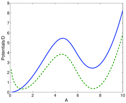
Refer to caption
Figure 7.12: Example of the potential V𝑉V (full) and the geometrically corrected potential 𝒱𝒱\mathcal{V} (dashed) for the SDQS in the coexistence regime. Notice for the corrected potential the logarithmic divergence in the origin.
Evaluation of the αisubscript𝛼𝑖\alpha_{i} and βisubscript𝛽𝑖\beta_{i} functions

We evaluate the αisubscript𝛼𝑖\alpha_{i} and βisubscript𝛽𝑖\beta_{i} functions numerically. Fortunately there is a rather natural discretization of the operators that compose the α𝛼\alpha and β𝛽\beta. This discretization is given by the operator 𝒫ϕcosϕsubscript𝒫italic-ϕitalic-ϕ\mathcal{P}_{\phi}\cos\phi that opens the operator string of all the components and that can be considered as a sort of Fourier transform of the function that follows. We specify better the concept and the method by reducing explicitly to the “numerical form” the contributions α0subscript𝛼0\alpha_{0} and α2subscript𝛼2\alpha_{2}:

α0=𝒫ϕcosϕG^0Γα2=𝒫ϕcosϕG^0Γg^0𝒬ϕP(G^0Γ)subscript𝛼0subscript𝒫italic-ϕitalic-ϕsubscript^𝐺0subscriptΓsubscript𝛼2subscript𝒫italic-ϕitalic-ϕsubscript^𝐺0subscriptΓsubscript^𝑔0subscript𝒬italic-ϕsubscript𝑃subscript^𝐺0subscriptΓ\begin{split}\alpha_{0}=&\mathcal{P}_{\phi}\cos\phi\hat{G}_{0}\Gamma_{-}\\ \alpha_{2}=&\mathcal{P}_{\phi}\cos\phi\hat{G}_{0}\Gamma_{-}\hat{g}_{0}\mathcal{Q}_{\phi}\partial_{P}(\hat{G}_{0}\Gamma_{-})\\ \end{split} (7.112)

where we remind G^0=(ϕ+Γ+)1subscript^𝐺0superscriptsubscriptitalic-ϕsubscriptΓ1\hat{G}_{0}=(\partial_{\phi}+\Gamma_{+})^{-1}. We define the function G(A,ϕ)G^0Γ(A,ϕ)𝐺𝐴italic-ϕsubscript^𝐺0subscriptΓ𝐴italic-ϕG(A,\phi)\equiv\hat{G}_{0}\Gamma_{-}(A,\phi). If G~n(A)subscript~𝐺𝑛𝐴\tilde{G}_{n}(A) is the discrete Fourier transform of G𝐺G (periodic function of ϕitalic-ϕ\phi)

G~n(A)=12π02πG(A,ϕ)einϕsubscript~𝐺𝑛𝐴12𝜋superscriptsubscript02𝜋𝐺𝐴italic-ϕsuperscript𝑒𝑖𝑛italic-ϕ\tilde{G}_{n}(A)=\frac{1}{2\pi}\int_{0}^{2\pi}G(A,\phi)e^{in\phi} (7.113)

with n𝑛n\in\mathbb{Z}, then we can easily recognize the Fourier transform in the definition of α0subscript𝛼0\alpha_{0} and write:

α0(A)=12(G~1+G~1)subscript𝛼0𝐴12subscript~𝐺1subscript~𝐺1\alpha_{0}(A)=\frac{1}{2}(\tilde{G}_{1}+\tilde{G}_{-1}) (7.114)

We still need to identify the structure of the functions G~n(A)subscript~𝐺𝑛𝐴\tilde{G}_{n}(A). It is useful for this purpose to calculate the Fourier transform of the functions Γ+subscriptΓ\Gamma_{+} and ΓsubscriptΓ\Gamma_{-} and define the vectors Γ¯~+subscript~¯Γ\tilde{\bar{\Gamma}}_{+} and Γ¯~subscript~¯Γ\tilde{\bar{\Gamma}}_{-} whose components are:

(Γ¯~+)n=Γω[Jn(2iA)+Jn(2iA)](Γ¯~)n=Γω[Jn(2iA)Jn(2iA)]subscriptsubscript~¯Γ𝑛Γ𝜔delimited-[]subscript𝐽𝑛2𝑖𝐴subscript𝐽𝑛2𝑖𝐴subscriptsubscript~¯Γ𝑛Γ𝜔delimited-[]subscript𝐽𝑛2𝑖𝐴subscript𝐽𝑛2𝑖𝐴\begin{split}(\tilde{\bar{\Gamma}}_{+})_{n}=\frac{\Gamma}{\omega}[J_{n}(-2iA)+J_{n}(2iA)]\\ (\tilde{\bar{\Gamma}}_{-})_{n}=\frac{\Gamma}{\omega}[J_{n}(-2iA)-J_{n}(2iA)]\end{split} (7.115)

where we have assumed for simplicity that ΓL=ΓR=ΓsubscriptΓ𝐿subscriptΓ𝑅Γ\Gamma_{L}=\Gamma_{R}=\Gamma and the Bessel function Jn(z)subscript𝐽𝑛𝑧J_{n}(z) is defined by:

Jn(z)=12π02πeinϕ+izsinϕ𝑑ϕsubscript𝐽𝑛𝑧12𝜋superscriptsubscript02𝜋superscript𝑒𝑖𝑛italic-ϕ𝑖𝑧italic-ϕdifferential-ditalic-ϕJ_{n}(z)=\frac{1}{2\pi}\int_{0}^{2\pi}e^{in\phi+iz\sin\phi}d\phi (7.116)

At the operator level we can write:

Γ(A,ϕ)=[ϕ+Γ+(A,ϕ)]G(A,ϕ)subscriptΓ𝐴italic-ϕdelimited-[]subscriptitalic-ϕsubscriptΓ𝐴italic-ϕ𝐺𝐴italic-ϕ\Gamma_{-}(A,\phi)=[\partial_{\phi}+\Gamma_{+}(A,\phi)]G(A,\phi) (7.117)

We take the Fourier transform in ϕitalic-ϕ\phi on both sides and we obtain:

(Γ¯~)n=m=[inδmn+(Γ¯¯~+)nmMnm]G~msubscriptsubscript~¯Γ𝑛superscriptsubscript𝑚delimited-[]subscript𝑖𝑛subscript𝛿𝑚𝑛subscriptsubscript~¯¯Γ𝑛𝑚subscript𝑀𝑛𝑚subscript~𝐺𝑚(\tilde{\bar{\Gamma}}_{-})_{n}=\sum_{m=-\infty}^{\infty}[\underbrace{in\delta_{mn}+(\tilde{\bar{\bar{\Gamma}}}_{+})_{nm}}_{\displaystyle M_{nm}}]\tilde{G}_{m} (7.118)

where we have defined the matrix (Γ¯¯~+)nm(Γ¯~+)nmsubscriptsubscript~¯¯Γ𝑛𝑚subscriptsubscript~¯Γ𝑛𝑚(\tilde{\bar{\bar{\Gamma}}}_{+})_{nm}\equiv(\tilde{\bar{\Gamma}}_{+})_{n-m} and the matrix M𝑀M. Finally we also define the Fourier transform of the cosine C¯=[,12,0,12,]T¯𝐶superscript12012𝑇\bar{C}=[\ldots,\frac{1}{2},0,\frac{1}{2},\ldots]^{T} with the 1/2121/2 in position ±1plus-or-minus1\pm 1 and we write the α0subscript𝛼0\alpha_{0} function in the compact numerical form:

α0=(C¯,M1Γ¯~)subscript𝛼0¯𝐶superscript𝑀1subscript~¯Γ\alpha_{0}=(\bar{C},M^{-1}\tilde{\bar{\Gamma}}_{-}) (7.119)

where the symbol (,)(\bullet,\bullet) indicates the scalar product between the two vectors. All the vectors must be truncated in the numerical evaluation, but fortunately the Bessel functions Jnsubscript𝐽𝑛J_{n} decay fast with n𝑛n and typically we verified numerical convergence taking only 40 terms around the zero position of the discrete Fourier transform “momentum space”.

If the derivation of the numerical form for α0subscript𝛼0\alpha_{0} is revealing the spirit of the calculation, the α2subscript𝛼2\alpha_{2} case contains instead some of the typical “tricks”. We start from the definition (7.112) and express the differential operator Psubscript𝑃\partial_{P} in polar coordinates. We obtain:

α2=𝒫ϕcosϕG^0Γg^0𝒬ϕ(sinϕAϕ+cosϕA)G^0Γsubscript𝛼2subscript𝒫italic-ϕitalic-ϕsubscript^𝐺0subscriptΓsubscript^𝑔0subscript𝒬italic-ϕitalic-ϕ𝐴subscriptitalic-ϕitalic-ϕsubscript𝐴subscript^𝐺0subscriptΓ\alpha_{2}=\mathcal{P}_{\phi}\cos\phi\hat{G}_{0}\Gamma_{-}\hat{g}_{0}\mathcal{Q}_{\phi}\left(-\frac{\sin\phi}{A}\partial_{\phi}+\cos\phi\partial_{A}\right)\hat{G}_{0}\Gamma_{-} (7.120)

We absorb the partial derivative ϕsubscriptitalic-ϕ\partial_{\phi} with the identification:

ϕ=G^01Γ+subscriptitalic-ϕsuperscriptsubscript^𝐺01subscriptΓ\partial_{\phi}=\hat{G}_{0}^{-1}-\Gamma_{+} (7.121)

Another important element is the combination g^0𝒬ϕsubscript^𝑔0subscript𝒬italic-ϕ\hat{g}_{0}\mathcal{Q}_{\phi}. It is important to study the Fourier transform of such an operator. Since g^0=(ϕ)1subscript^𝑔0superscriptsubscriptitalic-ϕ1\hat{g}_{0}=(\partial_{\phi})^{-1} we obtain:

(g^0)mn=inδnmsubscriptsubscript^𝑔0𝑚𝑛𝑖𝑛subscript𝛿𝑛𝑚(\hat{g}_{0})_{mn}=-\frac{i}{n}\delta_{nm} (7.122)

The singularity for n=0𝑛0n=0 is cured by the projector 𝒬ϕsubscript𝒬italic-ϕ\mathcal{Q}_{\phi} that removes the 0thsuperscript0th0^{\rm th} component in the Fourier transform of the vector on which it is acting. We call for this reason the combination g^0𝒬ϕsubscript^𝑔0subscript𝒬italic-ϕ\hat{g}_{0}\mathcal{Q}_{\phi} the pseudoinverse222222From the arguments above is clear that g^0𝒬ϕ𝒬ϕg^0𝒬ϕsubscript^𝑔0subscript𝒬italic-ϕsubscript𝒬italic-ϕsubscript^𝑔0subscript𝒬italic-ϕ\hat{g}_{0}\mathcal{Q}_{\phi}\equiv\mathcal{Q}_{\phi}\hat{g}_{0}\mathcal{Q}_{\phi}. of the differential operator ϕsubscriptitalic-ϕ\partial_{\phi} and we use the symbol (ϕ1)PSsubscriptsuperscriptsubscriptitalic-ϕ1𝑃𝑆(\partial_{\phi}^{-1})_{PS}.

The last problem that must be faced is the differential operator Asubscript𝐴\partial_{A} that we always encounter in the expression AGsubscript𝐴𝐺\partial_{A}G. Using the definition of G𝐺G and the results obtained in the evaluation of α0subscript𝛼0\alpha_{0} we can write:

AG~=M1AΓ¯~M1A(M)M1Γ¯~subscript𝐴~𝐺superscript𝑀1subscript𝐴subscript~¯Γsuperscript𝑀1subscript𝐴𝑀superscript𝑀1subscript~¯Γ\partial_{A}\tilde{G}=M^{-1}\partial_{A}\tilde{\bar{\Gamma}}_{-}-M^{-1}\partial_{A}(M)M^{-1}\tilde{\bar{\Gamma}}_{-} (7.123)

For the matrix M𝑀M and the vector Γ¯~subscript~¯Γ\tilde{\bar{\Gamma}}_{-} we have the explicit formulation in terms of the Bessel functions. Using the recursive relation between the functions J𝐽J and their derivatives

zJn(z)=12[Jn1(z)Jn+1(z)]subscript𝑧subscript𝐽𝑛𝑧12delimited-[]subscript𝐽𝑛1𝑧subscript𝐽𝑛1𝑧\partial_{z}J_{n}(z)=\frac{1}{2}[J_{n-1}(z)-J_{n+1}(z)] (7.124)

we obtain:

(AM)mn=iΓω[Jnm+1(2iA)Jnm1(2iA)Jnm+1(+2iA)+Jnm1(+2iA)](AΓ¯~)n=iΓω[Jn+1(2iA)Jn1(2iA)+Jn+1(+2iA)Jn1(+2iA)]=(AΓ¯¯~)n0subscriptsubscript𝐴𝑀𝑚𝑛𝑖Γ𝜔delimited-[]subscript𝐽𝑛𝑚12𝑖𝐴subscript𝐽𝑛𝑚12𝑖𝐴subscript𝐽𝑛𝑚12𝑖𝐴subscript𝐽𝑛𝑚12𝑖𝐴subscriptsubscript𝐴subscript~¯Γ𝑛𝑖Γ𝜔delimited-[]subscript𝐽𝑛12𝑖𝐴subscript𝐽𝑛12𝑖𝐴subscript𝐽𝑛12𝑖𝐴subscript𝐽𝑛12𝑖𝐴subscriptsubscript𝐴subscript~¯¯Γ𝑛0\begin{split}(\partial_{A}M)_{mn}=\frac{i\Gamma}{\omega}[&J_{n-m+1}(-2iA)-J_{n-m-1}(-2iA)\\ -&J_{n-m+1}(+2iA)+J_{n-m-1}(+2iA)]\\ (\partial_{A}\tilde{\bar{\Gamma}}_{-})_{n}=\frac{i\Gamma}{\omega}[&J_{n+1}(-2iA)-J_{n-1}(-2iA)\\ +&J_{n+1}(+2iA)-J_{n-1}(+2iA)]=(\partial_{A}\tilde{\bar{\bar{\Gamma}}}_{-})_{n0}\end{split} (7.125)

The “numerical form” of the function α2subscript𝛼2\alpha_{2} reads:

α2=1A(C¯,M1Γ¯¯~(ϕ)PS1(S¯¯Γ¯~S¯¯Γ¯¯~+G~AC¯¯M1(AΓ¯~A(M)G~)))subscript𝛼21𝐴¯𝐶superscript𝑀1subscript~¯¯Γsubscriptsuperscriptsubscriptitalic-ϕ1𝑃𝑆¯¯𝑆subscript~¯Γ¯¯𝑆subscript~¯¯Γ~𝐺𝐴¯¯𝐶superscript𝑀1subscript𝐴subscript~¯Γsubscript𝐴𝑀~𝐺\begin{split}\alpha_{2}=-\frac{1}{A}\Big{(}\bar{C},\,&M^{-1}\tilde{\bar{\bar{\Gamma}}}_{-}(\partial_{\phi})^{-1}_{PS}\big{(}\bar{\bar{S}}\tilde{\bar{\Gamma}}_{-}-\bar{\bar{S}}\tilde{\bar{\bar{\Gamma}}}_{+}\tilde{G}\\ &-A\bar{\bar{C}}M^{-1}(\partial_{A}\tilde{\bar{\Gamma}}_{-}-\partial_{A}(M)\tilde{G})\big{)}\Big{)}\end{split} (7.126)

where we have also introduced the sin\sin and cos\cos Fourier matrices:

S¯¯=12i(010101010),C¯¯=12(010101010)formulae-sequence¯¯𝑆12𝑖matrix010101010¯¯𝐶12matrix010101010\bar{\bar{S}}=\frac{1}{2i}\begin{pmatrix}\phantom{-}0&\phantom{-}1&0&\cdots\\ -1&\phantom{-}0&1&\cdots\\ \phantom{-}0&-1&0&\ddots\\ \phantom{-}\vdots&\phantom{-}\vdots&\ddots&\ddots\\ \end{pmatrix},\quad\bar{\bar{C}}=\frac{1}{2}\begin{pmatrix}0&1&0&\cdots\\ 1&0&1&\cdots\\ 0&1&0&\ddots\\ \vdots&\vdots&\ddots&\ddots\\ \end{pmatrix} (7.127)

The other α𝛼\alpha and β𝛽\beta functions are evaluated in a similar way and the calculations involved do not present any further complication.

7.3.3 Switching Rates

We have proven in section 7.3.2 that the SDQS dynamics in the coexistence regime can be described by a Kramers equation for the amplitude probability distribution 𝒲𝒲\mathcal{W} with a given potential 𝒱(𝒜)𝒱𝒜\mathcal{V(A)} and diffusion “constant” D(A)𝐷𝐴D(A). We then dedicated the last section to describe an affordable and reliable numerical evaluation of the α𝛼\alpha and β𝛽\beta functions that appear in the definition of the potential and diffusion constant. We are now able to identify completely the SDQS operating in the coexistence regime as a particular realization of the model for a dichotomous process between current modes presented in section 7.3.1. The shuttling and tunneling regimes with their characteristic currents are the two modes. Within the framework of the Kramers escape time theory we can now calculate the switching rates between these two modes.

The effective potential 𝒱𝒱\mathcal{V} that we obtained has for parameters that correspond to the coexistence regime, a typical double well bistable shape (Fig. 7.12). We assume for a while the diffusion constant to be independent of the amplitude A𝐴A. In this approximation the stationary solution of the equation (7.110) reads:

𝒲stat(A)=1𝒵exp(𝒱(A)D)superscript𝒲stat𝐴1𝒵𝒱𝐴𝐷\mathcal{W}^{\rm stat}(A)=\frac{1}{\mathcal{Z}}\exp\left(-\frac{\mathcal{V}(A)}{D}\right) (7.128)

where 𝒵𝒵\mathcal{Z} is the normalization 𝒵=0𝒲stat(A)𝑑A𝒵superscriptsubscript0superscript𝒲stat𝐴differential-d𝐴\mathcal{Z}=\int_{0}^{\infty}\mathcal{W}^{\rm stat}(A)dA. The probability distribution is concentrated around the minima of the potential and has a minimum in correspondence of the potential barrier. If this potential barrier is high enough (i.e. 𝒱max𝒱minDmuch-greater-thansubscript𝒱maxsubscript𝒱min𝐷\mathcal{V}_{\rm max}-\mathcal{V}_{\rm min}\gg D) we clearly identify two distinct states with definite average amplitude: the lower amplitude state corresponding to the tunneling regime and the higher to the shuttling (see fig. 7.13).
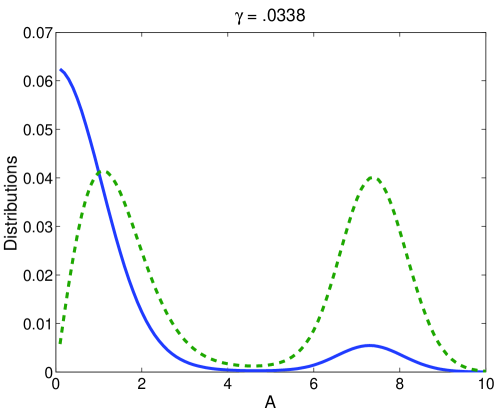
Refer to caption
Figure 7.13: Example of the stationary distribution W¯+statsuperscriptsubscript¯𝑊stat\bar{W}_{+}^{\rm stat} (full) and the amplitude distribution 𝒲statsuperscript𝒲stat\mathcal{W}^{\rm stat} (dashed) for the SDQS in the coexistence regime. The tunneling and shuttling states are in both cases well separated.

The Kramers equation (7.110) describes the coexistence regime of a SDQS by mapping it into a classical model for a particle moving in a bistable potential 𝒱𝒱\mathcal{V} with random forces described by the diffusion constant D𝐷D. It is this random force that allows the particle to overcome the barrier and jump between the two minima with definite rates. These rates are in the model for the SDQS the switching rates between the tunneling and shuttling mode ΓinsubscriptΓin\Gamma_{\rm in} and ΓoutsubscriptΓout\Gamma_{\rm out} that we introduced in section 6.3. The bistable potential model and the problem of calculating the average escape time (i.e. the average time necessary to leave one potential well) has been object of intense study because, despite its simplicity, it finds application, in different local variations, in many branches of science232323For a review on this problem– also called the exit problem or the escape time problem– see for example [48] or [49].. The first result on this problem, published in 1899 is the Arrhenius law for the chemical reaction rate κ𝜅\kappa (which Arrhenius attributed to van’t Hoff)

κ=ΩeEC/kBT𝜅Ωsuperscript𝑒subscript𝐸𝐶subscript𝑘𝐵𝑇\kappa=\Omega e^{-E_{C}/k_{B}T} (7.129)

where ECsubscript𝐸𝐶E_{C} is the activation energy, kBsubscript𝑘𝐵k_{B} the Boltzmann constant, T𝑇T is the absolute temperature and ΩΩ\Omega the attempt frequency or stearic factor. We base our derivation of the escape rates ΓinsubscriptΓin\Gamma_{\rm in} and ΓoutsubscriptΓout\Gamma_{\rm out} on the general treatment given in the book “The Fokker-Planck Equation Methods of Solution and Applications” by H. Risken [50].

Mean First Passage Time (MFPT) for a random variable

Given a stochastic variable ξ(t)𝜉𝑡\xi(t) (in our case the amplitude A(t)𝐴𝑡A(t)) we can ask the question when this variable first leaves a certain domain (e.g. one of the potential wells). This time is called first-passage time. For definiteness we choose the initial condition for the amplitude A𝐴A to be in the tunneling (lower amplitude) well and we ask when the amplitude is leaving for the first time the tunneling well to pass into the shuttling well. Since A𝐴A is a random variable, also the first-passage time is a random variable since it depends on the specific walk of the amplitude. We want to calculate the distribution function for the first-passage times and in particular its first moment, the mean-first passage time. This time would constitute in our specific case the inverse of the tunneling to shuttling switching rate ΓoutsubscriptΓout\Gamma_{\rm out}. We set the upper border Aoutsubscript𝐴outA_{\rm out} between the saddle point amplitude ASsubscript𝐴𝑆A_{S} and the shuttling amplitude Ashutsubscript𝐴shutA_{\rm shut}. We also set an arbitrary lower reflecting border in Aminsubscript𝐴minA_{\rm min}. 242424The exact position of the borders is not relevant as far as they are far from the minimum or the maximum of the potential.(see Fig. 7.14).
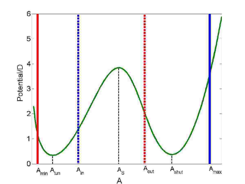
Refer to caption
Figure 7.14: Bistable effective potential for the SDQS coexistence regime. The important amplitudes for the calculation of the rates are indicated. The reflecting (full) and absorbing (dashed) borders for the calculation of the escape rates.

We define the probability density P(x,t|Atun,0)𝑃𝑥conditional𝑡subscript𝐴tun0P(x,t|A_{\rm tun},0) for the stochastic variable A(t)𝐴𝑡A(t) starting at t=0𝑡0t=0 with A(0)=Atun𝐴0subscript𝐴tunA(0)=A_{\rm tun} to be in x𝑥x at time t𝑡t without reaching the upper border Aoutsubscript𝐴outA_{\rm out}. It is possible to demonstrate [50] that the probability P𝑃P must obey the Kramers equation (7.110) if Amin<x<Aoutsubscript𝐴min𝑥subscript𝐴outA_{\rm min}<x<A_{\rm out}, is identically zero for xAout𝑥subscript𝐴outx\geq A_{\rm out} since the walks that touch the upper border are not taken into account and satisfy reflecting boundary conditions at the lower border, namely:

Pt=KP;P(x,0|Atun,0)=δ(xAtun)forAmin<x<AoutP(x,t|Atun,0)=0forx=Aoutxe𝒱(x)DP(x,t|Atun,0)|x=Amin=0\begin{split}&\frac{\partial P}{\partial t}=\mathcal{L}_{K}P;\quad P(x,0|A_{\rm tun},0)=\delta(x-A_{\rm tun})\quad\textrm{for}\quad A_{\rm min}<x<A_{\rm out}\\ &P(x,t|A_{\rm tun},0)=0\quad\textrm{for}\quad x=A_{\rm out}\\ &\partial_{x}e^{\frac{\mathcal{V}(x)}{D}}P(x,t|A_{\rm tun},0)|_{x=A_{\rm min}}=0\end{split} (7.130)

where Ksubscript𝐾\mathcal{L}_{K} is the Kramers’ Liouvillean of equation (7.110). The probability W(Atun,t)𝑊subscript𝐴tun𝑡W(A_{\rm tun},t) of realizations which have started at Atunsubscript𝐴tunA_{\rm tun} and which have not yet reached the upper boundary up to the time t𝑡t is given by:

W(Atun,t)=AminAoutP(x,t|Atun,0)𝑑x𝑊subscript𝐴tun𝑡superscriptsubscriptsubscript𝐴minsubscript𝐴out𝑃𝑥conditional𝑡subscript𝐴tun0differential-d𝑥W(A_{\rm tun},t)=\int_{A_{\rm min}}^{A_{\rm out}}P(x,t|A_{\rm tun},0)dx (7.131)

The probability dW𝑑𝑊-dW of those realizations which reach the upper boundary in the time interval (t,t+dt)𝑡𝑡𝑑𝑡(t,t+dt) thus reads

dW(Atun,t)=AminAoutP˙(x,t|Atun,0)𝑑x𝑑t𝑑𝑊subscript𝐴tun𝑡superscriptsubscriptsubscript𝐴minsubscript𝐴out˙𝑃𝑥conditional𝑡subscript𝐴tun0differential-d𝑥differential-d𝑡-dW(A_{\rm tun},t)=-\int_{A_{\rm min}}^{A_{\rm out}}\dot{P}(x,t|A_{\rm tun},0)dxdt (7.132)

The distribution w(T)𝑤𝑇w(T) function for the first passage time T is therefore given by

w(Atun,T)=dW(Atun,T)dT=AminAoutP˙(x,T|Atun,0)𝑑x𝑤subscript𝐴tun𝑇𝑑𝑊subscript𝐴tun𝑇𝑑𝑇superscriptsubscriptsubscript𝐴minsubscript𝐴out˙𝑃𝑥conditional𝑇subscript𝐴tun0differential-d𝑥w(A_{\rm tun},T)=-\frac{dW(A_{\rm tun},T)}{dT}=-\int_{A_{\rm min}}^{A_{\rm out}}\dot{P}(x,T|A_{\rm tun},0)dx (7.133)

The moments of the first-passage time distribution are

Tn(Atun)=0Tnw(Atun,T)𝑑T=AminAoutpn(x,Atun)𝑑xsubscript𝑇𝑛subscript𝐴tunsuperscriptsubscript0superscript𝑇𝑛𝑤subscript𝐴tun𝑇differential-d𝑇superscriptsubscriptsubscript𝐴minsubscript𝐴outsubscript𝑝𝑛𝑥subscript𝐴tundifferential-d𝑥T_{n}(A_{\rm tun})=\int_{0}^{\infty}T^{n}w(A_{\rm tun},T)dT=\int_{A_{\rm min}}^{A_{\rm out}}p_{n}(x,A_{\rm tun})dx (7.134)

where pn(x,Atun)subscript𝑝𝑛𝑥subscript𝐴tunp_{n}(x,A_{\rm tun}) is defined by

pn(x,Atun)=0TnP˙(x,T|Atun,0)𝑑Tsubscript𝑝𝑛𝑥subscript𝐴tunsuperscriptsubscript0superscript𝑇𝑛˙𝑃𝑥conditional𝑇subscript𝐴tun0differential-d𝑇p_{n}(x,A_{\rm tun})=-\int_{0}^{\infty}T^{n}\dot{P}(x,T|A_{\rm tun},0)dT (7.135)

We obviously have

p0(x,Atun)=0P˙(x,T|Atun,0)𝑑T=P(x,0|Atun,0)=δ(xAtun)subscript𝑝0𝑥subscript𝐴tunsuperscriptsubscript0˙𝑃𝑥conditional𝑇subscript𝐴tun0differential-d𝑇𝑃𝑥conditional0subscript𝐴tun0𝛿𝑥subscript𝐴tunp_{0}(x,A_{\rm tun})=-\int_{0}^{\infty}\dot{P}(x,T|A_{\rm tun},0)dT=P(x,0|A_{\rm tun},0)=\delta(x-A_{\rm tun}) (7.136)

Performing a partial integration gives the relation

pn(x,Atun)=n0Tn1P(x,T|Atun,0)𝑑Tsubscript𝑝𝑛𝑥subscript𝐴tun𝑛superscriptsubscript0superscript𝑇𝑛1𝑃𝑥conditional𝑇subscript𝐴tun0differential-d𝑇p_{n}(x,A_{\rm tun})=n\int_{0}^{\infty}T^{n-1}P(x,T|A_{\rm tun},0)dT (7.137)

Applying the Kramers’ Liouvillean Ksubscript𝐾\mathcal{L}_{K} to equation (7.137) we obtain the recursive relation:

K[pn(x,Atun)]=npn1(x,Atun)subscript𝐾delimited-[]subscript𝑝𝑛𝑥subscript𝐴tun𝑛subscript𝑝𝑛1𝑥subscript𝐴tun\mathcal{L}_{K}[p_{n}(x,A_{\rm tun})]=-np_{n-1}(x,A_{\rm tun}) (7.138)

and in particular

K[p1(x,Atun)]=δ(xAtun)subscript𝐾delimited-[]subscript𝑝1𝑥subscript𝐴tun𝛿𝑥subscript𝐴tun\mathcal{L}_{K}[p_{1}(x,A_{\rm tun})]=-\delta(x-A_{\rm tun}) (7.139)

In other words the function p1(x,Atun)subscript𝑝1𝑥subscript𝐴tunp_{1}(x,A_{\rm tun}) that enters the definition of the average first-passage time is the Green’s function of the Kramers’ Liouvillean Ksubscript𝐾\mathcal{L}_{K}. The Kramers’ Liouvillean can be written in the form:

K=DAe𝒱(A)DAe+𝒱(A)Dsubscript𝐾𝐷subscript𝐴superscript𝑒𝒱𝐴𝐷subscript𝐴superscript𝑒𝒱𝐴𝐷\mathcal{L}_{K}=D\partial_{A}e^{-\frac{\mathcal{V}(A)}{D}}\partial_{A}e^{+\frac{\mathcal{V}(A)}{D}} (7.140)

as can be easily proven by acting with the last partial derivative on the exponential. It is also possible252525Basically it is a double integration of equation (7.139). to give an analytic expression for the Green’s function p1(x,Atun)subscript𝑝1𝑥subscript𝐴tunp_{1}(x,A_{\rm tun}) of the Kramers’ Liouvillean Ksubscript𝐾\mathcal{L}_{K}:

p1(A,Atun)=1De𝒱(A)DAAoute𝒱(B)D[AAoutδ(CAtun)𝑑C]𝑑Bsubscript𝑝1𝐴subscript𝐴tun1𝐷superscript𝑒𝒱𝐴𝐷superscriptsubscript𝐴subscript𝐴outsuperscript𝑒𝒱𝐵𝐷delimited-[]superscriptsubscript𝐴subscript𝐴out𝛿𝐶subscript𝐴tundifferential-d𝐶differential-d𝐵p_{1}(A,A_{\rm tun})=\frac{1}{D}e^{-\frac{\mathcal{V}(A)}{D}}\int_{A}^{A_{\rm out}}e^{\frac{\mathcal{V}(B)}{D}}\left[\int_{A}^{A_{\rm out}}\delta(C-A_{\rm tun})dC\right]dB (7.141)

The mean-escape time from the tunneling well reads:

T1(Atun)=1DAminAout{e𝒱(A)DAAoute𝒱(B)D[AminBδ(CAtun)𝑑C]𝑑B}𝑑Asubscript𝑇1subscript𝐴tun1𝐷superscriptsubscriptsubscript𝐴minsubscript𝐴outsuperscript𝑒𝒱𝐴𝐷superscriptsubscript𝐴subscript𝐴outsuperscript𝑒𝒱𝐵𝐷delimited-[]superscriptsubscriptsubscript𝐴min𝐵𝛿𝐶subscript𝐴tundifferential-d𝐶differential-d𝐵differential-d𝐴T_{1}(A_{\rm tun})=\frac{1}{D}\int_{A_{\rm min}}^{A_{\rm out}}\left\{e^{-\frac{\mathcal{V}(A)}{D}}\int_{A}^{A_{\rm out}}e^{\frac{\mathcal{V}(B)}{D}}\left[\int_{A_{\rm min}}^{B}\delta(C-A_{\rm tun})dC\right]dB\right\}dA (7.142)

The escape time from the shuttling well can be calculated exactly in the same way using Ashutsubscript𝐴shutA_{\rm shut} as starting point for the random process and Ainsubscript𝐴inA_{\rm in} and Amaxsubscript𝐴maxA_{\rm max} as boundaries (see Fig. 7.14). The calculation of the integrals in (7.142) can be simplified considering that the integrand has a sharp maximum in the region (A,B)(Atun,AS)𝐴𝐵subscript𝐴tunsubscript𝐴S(A,B)\approx(A_{\rm tun},A_{\rm S}) due to the behaviour of the effective potential 𝒱𝒱\mathcal{V} around those two points. The escape time from the shuttling well can be calculated in a similar way. We obtain in the end the switching rates:

Γout=D(AtunAout𝑑Be𝒱(B)DAminB𝑑Ae𝒱(A)D)1Γin=D(AinAshut𝑑Be𝒱(B)DBAmax𝑑Ae𝒱(A)D)1subscriptΓout𝐷superscriptsuperscriptsubscriptsubscript𝐴tunsubscript𝐴outdifferential-d𝐵superscript𝑒𝒱𝐵𝐷superscriptsubscriptsubscript𝐴min𝐵differential-d𝐴superscript𝑒𝒱𝐴𝐷1subscriptΓin𝐷superscriptsuperscriptsubscriptsubscript𝐴insubscript𝐴shutdifferential-d𝐵superscript𝑒𝒱𝐵𝐷superscriptsubscript𝐵subscript𝐴maxdifferential-d𝐴superscript𝑒𝒱𝐴𝐷1\begin{split}\Gamma_{\rm out}&=D\left(\int_{A_{\rm tun}}^{A_{\rm out}}dB\,e^{\frac{{\mathcal{V}}(B)}{D}}\int_{A_{\rm min}}^{B}dA\,e^{-\frac{{\mathcal{V}}(A)}{D}}\right)^{-1}\\ \Gamma_{\rm in}&=D\left(\int_{A_{\rm in}}^{A_{\rm shut}}dB\,e^{\frac{{\mathcal{V}}(B)}{D}}\int_{B}^{A_{\rm max}}dA\,e^{-\frac{{\mathcal{V}}(A)}{D}}\right)^{-1}\\ \end{split} (7.143)

We recall here the equation for the current and the Fano factor for a dichotomous process inserting now the particular currents and switching rates characteristic of the SDQS coexistence regime:

Istat=IshΓout+ItunΓinΓin+ΓoutF=S(0)Istat=2(IshItun)2IshΓout+ItunΓinΓinΓout(Γin+Γout)2superscript𝐼statsubscript𝐼shsubscriptΓoutsubscript𝐼tunsubscriptΓinsubscriptΓinsubscriptΓout𝐹𝑆0superscript𝐼stat2superscriptsubscript𝐼shsubscript𝐼tun2subscript𝐼shsubscriptΓoutsubscript𝐼tunsubscriptΓinsubscriptΓinsubscriptΓoutsuperscriptsubscriptΓinsubscriptΓout2\begin{split}I^{\rm stat}&=\frac{I_{\rm sh}\Gamma_{\rm out}+I_{\rm tun}\Gamma_{\rm in}}{\Gamma_{\rm in}+\Gamma_{\rm out}}\\ F&=\frac{S(0)}{I^{\rm stat}}=2\frac{(I_{\rm sh}-I_{\rm tun})^{2}}{I_{\rm sh}\Gamma_{\rm out}+I_{\rm tun}\Gamma_{\rm in}}\frac{\Gamma_{\rm in}\Gamma_{\rm out}}{(\Gamma_{\rm in}+\Gamma_{\rm out})^{2}}\end{split} (7.144)

They represent, together with the stationary distribution

𝒲stat(A)=1𝒵exp(𝒱(A)D)superscript𝒲stat𝐴1𝒵𝒱𝐴𝐷\mathcal{W^{\rm stat}}(A)=\frac{1}{\mathcal{Z}}\exp\left(-\frac{\mathcal{V}(A)}{D}\right) (7.145)

the starting point for a quantitative comparison between the simplified model and the full description.

7.3.4 Comparison

The classical (but “noisy”) limit

The comparison between the dichotomous process model and the full description for the coexistence regime is based, as for the other regimes, on the three investigation tools: phase-space distribution, current and current-noise.

The phase space distribution is the most sensitive method to compare the model and the full description. One of the basic procedures adopted in the derivation of the Kramers equation (7.110) is the expansion to second order in the small parameters (7.96). In order to test the reliability of the model we simplify as much as possible the description reducing the model to a classical description: namely taking the zero limit for the parameter (x0λ)subscript𝑥0𝜆\left(\frac{x_{0}}{\lambda}\right). We realize physically this condition assuming a large temperature and a tunneling length λ𝜆\lambda of the order of the thermal length λth=kBTmω2subscript𝜆thsubscript𝑘𝐵𝑇𝑚superscript𝜔2\lambda_{\rm th}=\sqrt{\frac{k_{B}T}{m\omega^{2}}}. We partially discussed this limit in the previous chapters. Also the full description is slightly changed, but not qualitatively: the three regimes are still clearly present with their characteristics. The numerical calculation is though based on a totally different approach262626The continued fraction method was applied. See for example [50] for the application of this method to the solution of Fokker-Planck equations. The code was developed by Dr. T. Novotný..
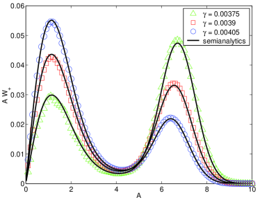
Refer to caption
Figure 7.15: Stationary amplitude probability distribution 𝒲𝒲\mathcal{W} for the SDQS in the coexistence regime. We compare the results obtained from the simplified model (full line) and from the full description (circles, triangles and squares). These results are obtained in the classical high temperature regime kBTωmuch-greater-thansubscript𝑘𝐵𝑇Planck-constant-over-2-pi𝜔k_{B}T\gg\hbar\omega. The amplitude is measured in units of λth=kBTmω2subscript𝜆thsubscript𝑘𝐵𝑇𝑚superscript𝜔2\lambda_{\rm th}=\sqrt{\frac{k_{B}T}{m\omega^{2}}}. The mechanical damping γ𝛾\gamma in units of the mechanical frequency ω𝜔\omega. The other parameter values are d=0.05λth𝑑0.05subscript𝜆thd=0.05\lambda_{\rm th} and Γ=0.015ωΓ0.015𝜔\Gamma=0.015\omega, λ=2λth𝜆2subscript𝜆th\lambda=2\lambda_{\rm th}.

In figures 7.15, 7.16 and 7.17 we present respectively the results for the stationary Wigner function, the current and the Fano factor in the semiclassical approximation and full description.
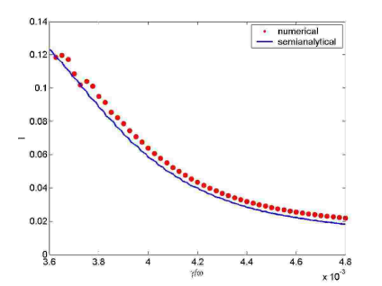
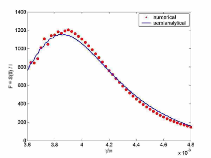
Refer to caption
Figure 7.16: Current in the coexistence regime of SDQS. Comparison between semianalytical and full numerical description. For the parameter values see Fig. 7.15.
Refer to caption
Figure 7.17: Fano factor in the coexistence regime of SDQS. Comparison between semianalytical and full numerical description. For the parameter values see Fig. 7.15.
The quantum limit

The coexistence regime in the parameters corner typically presented in this thesis (e.g. Fig. 5.5) is not captured by the model we introduced. The concept of elimination of the fast dynamics is still correct, but the small parameters expansion fails. The effective potential calculated from a second order expansion still gives the position of the ring structure with reasonable accuracy but the overall stationary Wigner function is not reproduced due to a non convergent diffusion function D(A)𝐷𝐴D(A). It is clear that we need to consider higher order terms in the parameter (x0/λ)2superscriptsubscript𝑥0𝜆2(x_{0}/\lambda)^{2}. This represents nevertheless a fundamental problem since it would produce terms with higher order derivatives with respect to the amplitude A𝐴A in the Fokker-Planck equation and consequently, to our knowledge, the break down of the escape time theory.

It has nevertheless been demonstrated with the help of the higher cumulants of the current that the dichotomous process description of the coexistence regime is valid also more in the quantum regime (λ=1.5x0𝜆1.5subscript𝑥0\lambda=1.5x_{0}), the only necessary condition being a separation of the ring and dot structures in the stationary Wigner function distribution [51].

Motivated by the fact that the effective potential was able to give the correct position of the shuttling ring we used the diffusion constant as a fitting parameter. The current and the Fano factor are very nicely reproduced in terms of a fitted diffusion constant approximately doubled with respect to the one calculated at zero temperature with no (x0λ)4superscriptsubscript𝑥0𝜆4\left(\frac{x_{0}}{\lambda}\right)^{4} corrections272727Even if at this level it could appear premature we wonder if this correction can be attributed to an effective temperature felt by the oscillator in contact with the electrical system lead-dot-lead far from equilibrium. A. Armour et al. support this hypothesis in similar devices [40] even if in slightly different regimes. (Figs. 7.18 and 7.19).
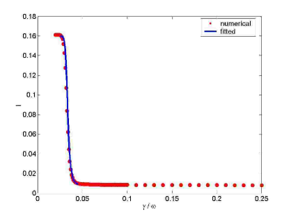
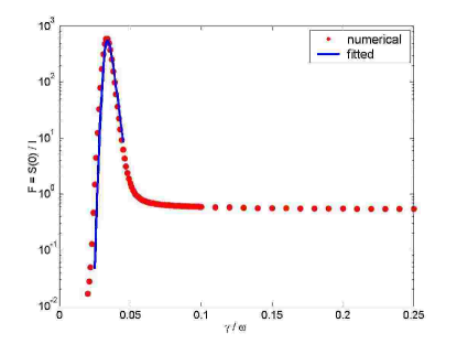
Refer to caption
Figure 7.18: Current in the coexistence regime of SDQS. Comparison between semianalytical description with an effective fitted diffusion constant (see the text for explanation) and full numerical description. The parameter values are Γ=0.01ωΓ0.01𝜔\Gamma=0.01\omega, λ=2x0𝜆2subscript𝑥0\lambda=2x_{0}, d=0.5x0𝑑0.5subscript𝑥0d=0.5x_{0}, T=0𝑇0T=0.
Refer to caption
Figure 7.19: Fano factor in the coexistence regime of SDQS. Comparison between semianalytical description with an effective fitted diffusion constant (see the text for explanation) and full numerical description. The parameter values are Γ=0.01ωΓ0.01𝜔\Gamma=0.01\omega, λ=2x0𝜆2subscript𝑥0\lambda=2x_{0}, d=0.5x0𝑑0.5subscript𝑥0d=0.5x_{0}, T=0𝑇0T=0.

The full numerical description presented in this thesis is relatively fragile with respect to the modification of the tunneling length282828We refer to changes of the tunneling length of one order of magnitude. at least for two reasons: the enlargement of the shuttling amplitude enlarges the number of oscillator states relevant for the dynamics to untractable numbers; the preconditioning loses effectiveness and the problem is not convergent. For this reason we are (still) lacking a numerical benchmark for the intermediate range of values of the tunneling length λ>x0𝜆subscript𝑥0\lambda>x_{0} but which is still non-classical where a second order expansion in the small parameter (x0λ)2superscriptsubscript𝑥0𝜆2\left(\frac{x_{0}}{\lambda}\right)^{2} is probably a good approximation.

Chapter 8 Conclusions

We summarize in this chapter the main results presented in the thesis. The richness of the shuttle model still leaves many points open in the description and understanding of the device dynamics. We close the chapter listing some of the open questions that could encourage a continuation of the present work.

8.1 Summary

We analyzed in this thesis the dynamics of two different shuttle devices: the single- and the triple-dot quantum shuttles. Shuttle devices are nanoelectromechanical systems (NEMS) in which an oscillating quantum dot can transfer electrons one per cycle from source to drain lead. The dynamics of such devices is the result of a strong interplay between their mechanical and electrical degrees of freedom.

The electrical dynamics is permeated of quantum effects: electrons can go from the source to the quantum dot and finally to the drain lead only via tunneling events; the small capacitance of the oscillating dot and the corresponding large charging energy reveals the discrete nature of the electrical charge; finally the presence of three coupled quantum dots is also a source of coherent electrical dynamics in the TDQS. The small size of the device makes quantum effects important also for the mechanical degree of freedom. The resonance frequency in such small (and relatively stiff) devices can be in the order of GHz. Consequently the quantum of energy of the harmonic oscillator is comparable with other energies in the device.

For these reasons for the SDQS we developed quantum models: we extended for the SDQS the classical model proposed by Gorelik et al. [1] and we adopted for the TDQS the one already existing invented by A. Armour and A. MacKinnon [7].

Among the different approaches for the description of the dynamics of a quantum system we chose the Generalized Master Equation (GME). GME’s are particularly well-suited to study small open quantum systems (i.e. systems with a small number of degrees of freedom in contact with resevoirs but still conserving some coherent dynamics) since they neglect the many (irrelevant) degrees of freedom of the resevoirs still keeping track of the residual quantum coherencies of the small system.

The shuttle devices are small quantum systems in contact with two kinds of resevoirs: the leads and the thermal bath. The strength of the coupling is very different and calls for a different treatment. The weak coupling between the thermal bath and the mechanical degree of freedom of the device justifies the perturbation theory and the quantum-optical derivation of a GME in Born-Markov approximation. The tunneling coupling of the shuttling devices to their electrical baths (the leads) is not weak. It sets, on the contrary, the time scale of the electrical dynamics that in the shuttling regime is comparable with the period of the mechanical oscillations in the system. This strong coupling condition is realized by a tunneling amplitude modulated by the displacement of the quantum dot from the equilibrium position in the SDQS while is directly set by a model parameter in the TDQS. In order to handle the strong coupling we adopted the Gurvitz method for the derivation of the GME and extended the original formulation to take into account the mechanical degree of freedom.

The shuttle dynamics has, especially in the single dot device, an appealing simple classical interpretation and one can say that the name itself of “shuttle” suggests the idea of sequential and periodical loading, mechanical transport and unloading of electrons between a source and a drain lead. For this reason, while preserving the complete quantum treatment that we achieved with the GME, we wanted to keep as much as possible the intuitive classical picture and the possibility to handle the quantum-classical correspondence. The Wigner function distribution seemed to us a good answer to all these requirements. It allows a clear visualization of the numerical results obtained within the framework of the GME and it shows in its equation of motion (the Klein-Kramers equation) an explicit quantum-classical correspondence (expansion in powers of Planck-constant-over-2-pi\hbar) [34].

Having the methods for the analysis of the shuttle device dynamics we looked for investigation tools. We first realized that a clear finger-print of the shuttling regime that distinguishes it from other kinds of phonon assisted tunneling is the charge-position(momentum) correlation. The Wigner distribution function on the device phase space (i.e. also charge resolved to take into account the two electrical states of the quantum dot) is a perfect tool to visualize this property. The only problem with the Wigner distribution functions is that it seems very difficult (if not impossible) to access experimentally these functions. For this reason, with the guidance of the distribution function description, we investigated the electronic transport properties in the shuttle devices (more realistically measurable): first the stationary current and then the current-noise111There is already a work that, in the semiclassical regime, addresses the aspect of full counting statistics for these devices [5]. Results for the quantum case will soon appear [51].. A special rôle in the calculation of the current-noise for the SDQS was played by a specific characteristic of the GME obtained in the Gurvitz approach. In this method the information on the state of the leads in not completely traced out and the number n𝑛n of electrons that passed through the device after a specific time appears in the equation of motion for the so-called n𝑛n-resolved reduced density matrix.

With these tools we investigated the properties of the quantum shuttle devices. The sharp tunneling-shuttling transition found by Gorelik et al. for the semiclassical model turned into a smooth crossover. We also could recognize the onset of the shuttling regime triggered by quantum mechanical noise with no external electric field acting on the oscillating quantum dot. The shuttle regime also revealed the characteristic current quantization (in our set-up a saturation due to Coulomb blockade to one electron per cycle in the cleanest shuttling regime) and the extremely low noise typical of a quasi-deterministic transport regime. With all the three investigation tools we adopted we could recognize three operating regimes for the shuttle device: tunneling, shuttling and coexistence regime. They represent for the SDQS the whole scenario of possible dynamics. Part of the complexity of the TDQS is also captured in this scheme222For a further insight into this particular model see [7, 10, 12, 33]..

The specific separation of time scales in the different regimes allowed us to identify the relevant variables and describe each regime by a specific simplified model. In the tunneling (high damping) regime the mechanical degree of freedom is almost frozen and all the features revealed by the Wigner distribution, the current and the current noise can be reproduced with a resonant tunneling model with tunneling rates renormalized due to the movable quantum dot. Most of the features of the shuttling regime (self-sustained oscillations, charge-position correlation and current quantization) are captured by a simple model derived as the zero-noise limit of the full description. Finally for the coexistence regime we proposed a dynamical picture in terms of slow dichotomous switching between the tunneling and shuttling modes. This interpretation was mostly suggested by the presence in the stationary Wigner function distributions of both the characteristic features of the tunneling and shuttling dynamics and by a corresponding gigantic peak in the Fano factor. We based the derivation of the simplified model on the fast variables elimination from the Klein-Kramers equations for the Wigner function333The analytical derivation of the effective potential is an extension of the work done by Fedorets et al. [9]. and a consequent derivation of an effective bistable potential for the amplitude of the dot oscillation (the relevant slow variable in this regime).

8.2 Some open questions

During the developing of the present work many questions arose about possible phenomena to investigate in different shuttle devices or other possible regimes that the systems we investigate could exhibit in some other parameter corner that we did not reach. This questions could be of interest for example in understanding or proposing future experiments. We list them here as a spur for possible continuation of the present work sure that some of the theoretical tools presented in this thesis are definitely useful for those tasks.

  • The mechanical bath introduces decoherence in the mechanical degree of freedom, the leads in the electrical. Correlations are left (in the SDQS) only in the off-diagonal elements of the charge resolved density matrices. Can we imagine an electromechanical system that instead exhibits quantum coherence in the mechanical degree of freedom? Could we use the electromechanical interaction to “pump” continuously coherence in the device?

  • The stationary solution for the GME is incoherent. Is there any possibility to reduce the GME to an effective Master equation? We imagine that especially in the coexistence regime this could help to avoid the Wigner function small parameter expansion for the calculation of the effective bistable potential and lead directly to the calculation of the rates for the slow switching process. This would make the calculation of the parameters for the dichotomous process description much more general.

  • Taking into account the spin degrees of freedom and the Coulomb blockade the incoming bare rate should be considered as double with respect to the out going rate. This fact does not change qualitatively the picture since the switching is, in first approximation a non-dissipative process and the electrostatic force is a small perturbation of the oscillator restoring force. The mechanical trajectories are not significantly changed (maybe slightly decreased in radius) and only the symmetry between the two charged resolved Wigner functions is modified in favour of W11subscript𝑊11W_{11}: the dot is charged for a longer time. But what happens if we consider a spin dynamics on the dot due for example to a coupling to an external magnetic field444A partial answer to this questions is contained in the very recent paper by Fedorets et al. [47].?

  • At high bare injection rates (Γωmuch-greater-thanΓ𝜔\Gamma\gg\omega) the shuttle device is more stable and hardly leaves the tunneling regime. The mechanical motion cannot in fact follow the fast electrical forcing and the effect is generally uncorrelated resonant tunneling. Nevertheless at extremely low damping the shuttling regime arises. The transition is very different from the small injection rate shuttling instability: it is very smooth and the ring structure gradually emerges from the central fuzzy spot typical for the tunneling regime. The general question is: can we draw a phase diagram for shuttling devices as a function of their parameters?

  • A big issue regards the treatment of the bias in the quantum description. All our equations were derived in the limit of high external bias. We did not have access to this parameter and we used for this reason the mechanical damping as a control parameter. Is it possible to derive a GME at low bias and for strong couplings to the leads? Probably the dynamics will get non-Markovian and all kinds of coherent transport effects will also enter the game. We know from the semiclassical treatment that the shuttling instability should be present. Can we understand something new from the quantum treatment?

Bibliography

  • [1] L. Y. Gorelik, A. Isacsson, M. V. Voinova, B. Kasemo, R. I. Shekhter, and M. Jonson, Shuttle Mechanism for Charge Transfer in Coulomb Blockade Nanostructures, Phys. Rev. Lett. 80(20), 4526 (May 1998).
  • [2] A. Isacsson, L. Y. Gorelik, M. V. Voinova, B. Kasemo, R. I. Shekhter, and M. Jonson, Shuttle instability in self-assembled Coulomb blockade nanostructures, Physica B 255, 150–163 (December 1998).
  • [3] C. Weiss and W. Zwerger, Accuracy of a mechanical single-electron shuttle, Europhys. Lett. 47(1), 97–103 (July 1999).
  • [4] N. Nishiguchi, Gate voltage dependence of a single-electron transistor using the shuttle mechanism, Phys. Rev. B 65(3), 035403 (December 2001).
  • [5] F. Pistolesi, Full counting statistics of a charge shuttle, Phys. Rev. B 69(24), 245409 (June 2004).
  • [6] T. Nord and A. Isacsson, Impact of van der Waals forces on the classical shuttle instability, Phys. Rev. B 69(3), 35309 (January 2004).
  • [7] A. D. Armour and A. MacKinnon, Transport via a quantum shuttle, Phys. Rev. B 66(3), 035333 (July 2002).
  • [8] T. Novotný, A. Donarini, and A.-P. Jauho, Quantum Shuttle in Phase Space, Phys. Rev. Lett. 90(25), 256801 (June 2003).
  • [9] D. Fedorets, L. Y. Gorelik, R. I. Shekhter, and M. Jonson, Quantum Shuttle Phenomena in a Nanoelectromechanical Single-Electron Transistor, Phys. Rev. Lett. 92(16), 166801 (April 2004).
  • [10] A. Donarini and A.-P. Jauho, Shuttle instabilities: semiclassical phase analysis, Physica E 22(1–3), 721 (April 2004).
  • [11] A. Donarini, T. Novotný, and A.-P. Jauho, Quantum theory of shuttling instability in a movable quantum dot array, Semicond. Sci. Technol. 19(4), S430 (April 2004).
  • [12] C. Flindt, Current Noise in a 3-Dot Quantum Shuttle, Master’s thesis, MIC, Technical University of Denmark, March 2004.
  • [13] A. Romito, F. Plastina, and R. Fazio, Decoherence in a Cooper pair shuttle, Phys. Rev. B 68(14), 140502 (October 2003).
  • [14] A. Romito and Y. V. Nazarov, Full Counting Statistics of Cooper Pair Shuttling, cond-mat/0402412, February 2004.
  • [15] L. Y. Gorelik, A. Isacsson, Y. M. Galperin, R. I. Shekhter, and M. Jonson, Coherent transfer of Cooper pairs by a movable grain, Nature 411, 454 (May 2001).
  • [16] L. Y. Gorelik, R. I. Shekhter, M. Jonson, S. I. Kulinich, and V. M. Vinokur, Spin-Dependent Transport of Electrons in a Shuttle Structure, cond-mat/0402284, February 2004.
  • [17] A. Erbe, C. Weiss, W. Zwerger, and R. H. Blick, Nanomechanical Resonator Shuttling Single Electrons at Radio Frequencies, Phys. Rev. Lett. 87(9), 096106 (August 2001).
  • [18] H. Park, J. Park, A. K. L. Lim, E. H. Anderson, A. P. Alivisatos, and P. L. McEuen, Nanomechanical oscillations in a single-C60 transistor, Nature 407, 57 (September 2000).
  • [19] D. Fedorets, L. Y. Gorelik, R. I. Shekhter, and M. Jonson, Vibrational instability due to coherent tunneling of electrons, Europhys. Lett. 58(1), 99–104 (April 2002).
  • [20] D. Boese and H. Schoeller, Influence of nanomechanical properties on single-electron tunneling: A vibrating single-electron transistor, Europhys. Lett. 54(5), 668–674 (June 2001).
  • [21] K. D. McCarthy, N. Prokof’ev, and M. T. Tuominen, Incoherent dynamics of vibrating single-molecule transistors, Phys. Rev. B 67(24), 245415 (June 2003).
  • [22] T. Brandes and N. Lambert, Steering of a bosonic mode with a double quantum dot, Phys. Rev. B 67(12), 125323 (March 2003).
  • [23] T. Novotný, A. Donarini, C. Flindt, and A.-P. Jauho, Shot Noise of a Quantum Shuttle, Phys. Rev. Lett. 92(24), 248302 (June 2004).
  • [24] D. V. Scheible and R. Blick, Silicon nanopillars for mechanical single-electron transport, Appl. Phys. Lett. 84(23), 4632 (June 2004).
  • [25] E. Onofri and C. Destri, Istituzioni di Fisica Teorica, Carocci, first edition, 1998.
  • [26] K. Huang, Statistical Mechanics, John Wiley & Sons, second edition, 1987.
  • [27] C. W. Gardiner and P. Zoller, Quantum Noise, Springer, second edition, 2000.
  • [28] S. A. Gurvitz and Y. S. Prager, Microscopic derivation of rate equations for quantum transport, Phys. Rev. B 53(23), 15932–15942 (June 1996).
  • [29] M. R. Wegewijs and Y. V. Nazarov, Resonant tunneling through linear arrays of quantum dots, Phys. Rev. B 60(20), 14318 (November 1999).
  • [30] D. Kohen, C. C. Marston, and D. J. Tannor, Phase space approach to theories of quantum dissipation, J. Chem. Phys. 107(13), 5236 (October 1997).
  • [31] T. Eirola and O. Nevanlinna, Numerical linear algebra; iterative methods, Lecture notes, Helsinki University of Technology, 2003.
  • [32] G. H. Golub and C. F. V. Loan, Matrix Computations, The John Hopkins University Press, third edition, 1996.
  • [33] C. Flindt, T. Novotný, and A.-P. Jauho, Current noise in a vibrating quantum dot array, cond-mat/0405512, May 2004, accepted to PRB.
  • [34] M. Hillery, R. F. O’Connell, M. O. Scully, and E. P. Wigner, Distribution functions in physics: fundamentals, Phys. Rep. 106(3), 121 (1984).
  • [35] R. F. O’Connell and E. P. Wigner, Quantum-mechanical distribution functions: conditions for uniqueness, Phys. Lett. A 83A(4), 145 (1981).
  • [36] S. Braig and K. Flensberg, Vibrational sidebands and dissipative tunneling in molecular transistors, Phys. Rev. B 68(20), 205324 (November 2003).
  • [37] Y. M. Blanter and M. Büttiker, Shot noise in mesoscopic conductors, Physics Reports 336(1–2), 1–166 (September 2000).
  • [38] C. Beenakker and C. Schönenberger, Quantum Shot Noise, Physics Today 56(5), 37 (May 2003).
  • [39] A. Mitra, I. Aleiner, and A. J. Millis, Phonon effects in molecular transistors: Quantual and classical treatment, Phys. Rev. B 69(24), 245302 (June 2004).
  • [40] A. D. Armour, M. P. Blencowe, and Y. Zhang, Classical dynamics of a nano-mechanical resonator coupled to a single-electron transistor, Phys. Rev. B 69, 125313 (March 2004).
  • [41] N. M. Chtchelkatchev, W. Belzig, and C. Bruder, Charge transport through a SET with a mechanically oscillating island, cond-mat/0401486, January 2004.
  • [42] A. Isacsson and T. Nord, Low-frequency current noise of the single-electron shuttle, Europhys. Lett. 66(5), 708 (June 2004).
  • [43] B. Elattari and S. A. Gurvitz, Shot noise in coupled dots and the “fractional charges”, Phys. Lett. A 292, 289 (January 2002).
  • [44] H. Bruus and K. Flensberg, Many-Body Quantum Theory in Condensed Matter Physics, Oxford University Press, Oxford, 2003.
  • [45] J. H. Davies, P. Hyldgaard, S. Hershfield, and J. W. Wilkins, Classical theory of shot noise in resonant tunneling, Phys. Rev. B 46(15), 9620 (October 1992).
  • [46] H.-P. Breuer and F. Petruccione, The Theory of Open Quantum Systems, Oxford University Press, first edition, 2002.
  • [47] D. Fedorets, L. Y. Gorelik, R. I. Shekhter, and M. Jonson, Spintronics of a Nanoelectromechanical Shuttle, cond-mat/0408591, August 2004.
  • [48] T. Naeh, M. M. Klosek, B. J. Matkowsky, and Z. Schuss, A direct approach to the exit problem, SIAM J. Appl. Math. 50(2), 595 (April 1990).
  • [49] D. Ludwig, Persistence of dynamical systems under random perturbations, SIAM Review 17(4), 605 (October 1975).
  • [50] H. Risken, The Fokker-Planck Equation, Springer, Berlin, 1996.
  • [51] C. Flindt, T. Novotný, and A.-P. Jauho, Full counting statistics of nano-electromechanical systems, cond-mat/0410322, October 2004.