On-lattice coalescence and annihilation of immobile reactants in loopless lattices and beyond

Abstract

We study the behavior of the chemical reactions $A+A\to A+S$ and $A+A\to S+S$ (where the reactive species $A$ and the inert species $S$ are both assumed to be immobile) embedded on Bethe lattices of arbitrary coordination number $z$ and on a two-dimensional ($2D$) square lattice. For the Bethe lattice case, exact solutions for the coverage in the $A$ species in terms of the initial condition are obtained. In particular, our results hold for the important case of an infinite one-dimensional ($1D$) lattice ($z=2$). The method is based on an expansion in terms of conditional probabilities which exploits a Markovian property of these systems. Along the same lines, an approximate solution for the case of a $2D$ square lattice is developed. The effect of dilution in a random initial condition is discussed in detail, both for the lattice coverage and for the spatial distribution of reactants.

I Introduction

A rigorous description of the dynamics of the relevant macrovariables in reaction-diffusion systems requires a probabilistic multilevel approach retaining the essential features of the underlying many-body problem vkamp ; gard ; nicpr . In this coarse-grained picture, typical macrovariables such as concentrations are no longer deterministic, but rather stochastic quantities. In a number of typical situations, the equations governing the dynamics of the mean concentrations turn out to be identical with the classical law of mass action. In the absence of external asymmetries or of symmetry-breaking instabilities, the latter can be regarded as a mean-field (MF) law, in the sense that each part of the system is assumed to interact with the whole bulk at all times by means of an effective field which does not account for spatial effects.

The above classical approach can be regarded as a good approximation as long as the characteristic time associated with the mean free path is short compared to the mean reaction time within the typical interaction radius. This is only the case if the system is well mixed at all times, either through external stirring or through fast internal diffusion. The opposite situation corresponds to the diffusion-controlled limit, where each reactant typically explores a significant portion of space before undergoing a reactive collision, and the way in which reactants are distributed on a microscopic scale starts to become important for the determination of macrovariables such as global concentrations or, in the case of a lattice systems, the coverage in the different species. In such cases, classical MF approaches fail to describe the onset of inhomogeneous fluctuations induced by the intrinsic chemical noise of the system. Such fluctuations are nowadays directly observable at nanometric scales with the help of STM and FIM microscopy techniques such0 ; such1 and can be enhanced by specific geometric constraints and/or in low dimensions (e.g. catalytic surfaces), where external stirring is difficult and diffusion inefficient; eventually, they may give rise to non-classical effects such as memory of the initial condition, self-ordering phenomena, etc. havlin . Elucidating the role of geometry in this context is of great theoretical and practical interest in view of the recent progress in the development of nanoscale supports.

Fluctuation-induced effects become even stronger in systems with immobile reactants, the object of the present paper. The particular systems we shall investigate here are the on-lattice reactions $A+A\rightarrow A+S$ and $A+A\rightarrow S+S$ with nearest neighbor interactions, where $A$ and $S$ denote, respectively, a site occupied by the reactive species (“occupied site”) and the inert species (“empty site”), both assumed to be immobile. Popularly, these reactions are termed coalescence (CR) and annihilation reaction (AR) respectively. Various workers have intensively investigated the CR avrabursch ; Spou ; abad2 and the AR Spou ; Torn ; Lus ; Schut ; Gryn ; Fam2 in the diffusion-controlled limit. Besides a series of applications for nucleation and aggregation systems Leyv ; prov2 , the diffusion-controlled CR has also been recently used as a model for exciton fusion in polymers and molecular crystals kop0 ; kop1 ; privb , while the AR model provides a basic description for recombination processes and exciton annihilation Racz ; privb . In the immobile reactant limit, the AR model has been e.g. used to study free radical recombination on surfaces Jack , cyclization reactions in polymers cohen and colloid deposition problems Bart among other applications. Note the formal similarity of this model and models for dimer random sequential absorption (DRSA) Evans ; Dick . In such DRSA models, the deposition of a dimer on two empty sites is dual to the removal of two neighboring particles from the lattice upon reactions in the AR model, i.e. empty sites play the role of occupied sites and vice versa. There exists also a (less obvious) mapping between the CR model and a particular case of random monomer filling with nearest neighbor cooperativity kell ; mity ; fan . However, most studies concerning the above RSA models were performed for a fixed initial condition. Typically, the latter corresponds to a situation where all lattice sites are vacant, which in the dual picture of our model is equivalent to a fully covered lattice. In contrast, we shall consider here the general case in which the lattice is partially filled initially and study how this affects the subsequent dynamics and steady state of the system.

Previous studies have shown that in the immobile reactant limit the one-dimensional CR and AR models with nearest neighbor interactions are characterized by an exponential decay of the mean coverage $\theta(t)$ in the reactive species to a nonergodic set of invariant states, as opposed to the empty state predicted by the MF equation baras ; abad1 . In the present work, we extend these results to the case of a partially filled Bethe lattice with arbitrary coordination number. In such loopless lattices, the relevant hierarchy of probabilities can be truncated exactly using a shielding (Markovian) property of the conditional probabilities for the state of a given site. This method is used to generalize previous results by Evans Evans3 and by Majumdar and Privman Priv . Next, we treat the case of a $2D$ square lattice by performing an expansion based on the shortest unshielded path approximation developed by Nord and Evans for a series of RSA models Nord . The results for the asymptotic coverage are then compared with Monte Carlo (MC) simulations. The effect of the initial condition on the spatial ordering induced by the reaction is also discussed by studying the dynamical behavior of the conditional probabilities and the associated fluctuation correlations. In the last section, we summarize the main conclusions and outline possible extensions of our work.

II The CR and the AR model in Bethe lattices: exact solution via shielding property

As a starting point, we consider an ensemble of Bethe lattices with coordination number $z$ (the case $z=2$ corresponds to an infinite $1D$ lattice). In each lattice, sites are initially occupied at random with probability $p$ (equal to the initial lattice coverage $\theta(0)$). We then let the particles interact according to the CR (AR) scheme with nearest neighbor interactions specified above. By construction, the resulting statistical system will be translationally invariant at all times. Let us absorb the reaction rate $R$ into the time scale by introducing the dimensionless time variable $\tau\equiv R\,t$. Let us denote by $P_{k}(\tau)$ the probability that $k$ randomly chosen nearest neighbor sites in a given lattice are all simultaneously occupied ($k$-site cluster). The evolution equations for the ensemble probabilities $P_{k}$ read Priv

$$\frac{dP_{k}}{d\tau}=-(k-1)P_{k}-\frac{\nu}{2}(zk-2k+2)\,P_{k+1},\quad k=1,2,\ldots$$ (1)

where $\nu=1,2$ for the CR and the AR model, respectively.

The first term on the right hand side represents the destruction of a $k$-site cluster by interaction between two particles inside the cluster and is proportional to the number of internal bonds ($=k-1$ bonds). The second term represents the destruction of a $k$-site cluster due to the disappearance of a particle inside the cluster upon interaction with a neighboring particle just outside the cluster. Such an event is only possible if a $k+1$-site cluster preexists, implying that this term is proportional to $P_{k+1}$. Its coefficient is proportional to the number of bonds between the $k$ cluster sites and external neighboring sites (=$zk-2k+2$). The different value of $\nu$ stems from the fact that the $k$-site cluster is only destroyed if the particle vanishes upon interaction with a filled neighbor outside the cluster. In the CR case, this only happens one time out of two, since in a single event the particle inside the cluster has the same probability of vanishing as the neighbor particle outside the cluster.

We now seek a special solution of the hierarchy (1) corresponding to our initial condition. One easily check that in our case $P_{k}(0)=p^{k}$. As it turns out, the hierarchy can be exactly truncated after the first two equations

$$\frac{dP_{1}}{d\tau} = -\frac{\nu}{2}\,zP_{2},$$ (2a)

$$\frac{dP_{2}}{d\tau} = -P_{2}-\nu\,(z-1)P_{3}.$$ (2b)

Exact truncation is possible because of the existence of a special property for the quantity $Q_{\begin{picture}(25.0,20.0)\put(2.0,14.0){\circle*{4.0}}\put(8.0,14.0){\circle*{4.0}} \put(7.0,10.0){\line(1,4){2.5}} \put(12.0,14.0){\circle*{1.0}}\put(15.0,14.0){\circle*{1.0}}\put(18.0,14.0){\circle*{1.0}} \put(22.0,14.0){\circle*{4.0}} \put(21.0,10.0){\line(1,4){2.5}} \put(14.5,11.0){\makebox(0.0,0.0)[t]{$\underbrace{}$}} \put(16.0,-2.0){\makebox(0.0,0.0)[b]{\tiny k-times}} \end{picture}}(\tau)=P_{k+1}/P_{k}$, i.e. the conditional probability that a site is occupied given that its $k$ nearest neighbors along any irreversible path starting from the site are occupied. Here “” denotes an occupied site, while “” denotes a conditioning occupied site. Rewriting Eqs. (2) in terms of these probabilities, one has

$$\frac{d}{d\tau}\ln Q_{\begin{picture}(10.0,8.0)\put(4.0,2.0){\circle*{4.0}} \end{picture}} = -\,\nu\,\frac{z}{2}\,Q_{\begin{picture}(10.0,10.0)\put(2.0,4.0){\circle*{4.0}} \put(8.0,4.0){\circle*{4.0}} \put(7.0,0.0){\line(1,4){2.5}} \end{picture}},$$ (3a)

$$\frac{d}{d\tau}\ln Q_{\begin{picture}(10.0,10.0)\put(2.0,4.0){\circle*{4.0}} \put(8.0,4.0){\circle*{4.0}} \put(7.0,0.0){\line(1,4){2.5}} \end{picture}} = -1+\frac{\nu z}{2}Q_{\begin{picture}(10.0,10.0)\put(2.0,4.0){\circle*{4.0}} \put(8.0,4.0){\circle*{4.0}} \put(7.0,0.0){\line(1,4){2.5}} \end{picture}}-\nu\,(z-1)Q_{\begin{picture}(15.0,10.0)\put(2.0,4.0){\circle*{4.0}}\put(8.0,4.0){\circle*{4.0}}\put(14.0,4.0){\circle*{4.0}} \put(7.0,0.0){\line(1,4){2.5}}\put(13.0,0.0){\line(1,4){2.5}} \end{picture}},$$ (3b)

where the notation $Q_{\begin{picture}(10.0,8.0)\put(4.0,2.0){\circle*{4.0}} \end{picture}}\equiv P_{1}$ has been used. Now, in a Bethe lattice a conditioning site specified as occupied “shields”, i.e. clusters belonging to disjoint irreversible paths starting from the occupied site evolve independently of each other . As a consequence, one has Vette ; mity ; Evans3

$$Q_{\begin{picture}(10.0,10.0)\put(2.0,4.0){\circle*{4.0}} \put(8.0,4.0){\circle*{4.0}} \put(7.0,0.0){\line(1,4){2.5}} \end{picture}}=Q_{\begin{picture}(15.0,10.0)\put(2.0,4.0){\circle*{4.0}}\put(8.0,4.0){\circle*{4.0}}\put(14.0,4.0){\circle*{4.0}} \put(7.0,0.0){\line(1,4){2.5}}\put(13.0,0.0){\line(1,4){2.5}} \end{picture}}=Q_{\begin{picture}(22.0,10.0)\put(2.0,4.0){\circle*{4.0}}\put(8.0,4.0){\circle*{4.0}}\put(14.0,4.0){\circle*{4.0}}\put(20.0,4.0){\circle*{4.0}} \put(7.0,0.0){\line(1,4){2.5}}\put(13.0,0.0){\line(1,4){2.5}}\put(19.0,0.0){\line(1,4){2.5}} \end{picture}}\cdots,\quad\mbox{etc.}$$ (4)

i.e. the memory of the system is limited to the nearest neighbor site. In this sense, the subset of occupied sites can be said to display (first-order) spatial markovianity Malek .

Using the shielding property (4), Eqs. (3) become a closed two-variable system. Since the system is translationally invariant, the local probability $Q_{\begin{picture}(10.0,8.0)\put(4.0,2.0){\circle*{4.0}} \end{picture}}$ is identical with the global coverage $\theta$. The solution of Eqs. (3) reads

$$Q_{\begin{picture}(10.0,8.0)\put(4.0,2.0){\circle*{4.0}} \end{picture}}(\tau) = \theta(\tau)=p\,\left[1+\frac{(z-2)}{2}\,\nu\,p(1-e^{-\tau})\right]^{-z/(z-2)},$$ (5a)

$$Q_{\begin{picture}(10.0,10.0)\put(2.0,4.0){\circle*{4.0}} \put(8.0,4.0){\circle*{4.0}} \put(7.0,0.0){\line(1,4){2.5}} \end{picture}}(\tau) = \frac{p\,e^{-\tau}}{1+\frac{\textstyle(z-2)}{\textstyle 2}\,\nu\,p\,(1-e^{-\tau})}.$$ (5b)

Thus, the global coverage attains the asymptotic value

$$\theta_{S}=\theta(\infty)=p\,\left[1+\frac{z-2}{2}\,\nu\,p\right]^{-z/(z-2)}.$$ (6)

Regardless of the value of $z$, $\theta_{S}$ increases monotonically with increasing $p$ for the CR model, while in the AR model it follows a non-monotonic behavior with a universal maximum at $p=\frac{1}{2}$. This may be related to the fact that the mean asymptotic number of particles yielded by islands (=disconnected clusters) created by the ongoing reactions does not grow monotonically with the island size, as opposed to the CR case prov3 ; thes . Thus, larger islands characteristic of high values of the initial coverage $p$ may eventually yield a lower number of particles than smaller ones. In particular two-particle islands are known to disappear from the system, while one-particle islands survive forever.

As expected, $\theta_{S}$ decreases strongly as a function of $z$, approaching a zero value when $z\to\infty$. This is in agreement with our intuitive expectation that the system must approach the classical MF prediction with increasing connectivity.

Eq. (5a) generalizes previous results by Evans for the DRSA problem equivalent to the $p=1$ case Evans3 and Majumdar and Privman for the $\nu=2$ case Priv . The special case of a $1D$ lattice is obtained when $z\to 2^{+}$. In this limit, Eqs. (5) become

$$\theta(\tau) = p\,\exp{(\,\nu\,p\,[e^{-\tau}-1]\,)},$$ (7a)

$$Q_{\begin{picture}(10.0,10.0)\put(2.0,4.0){\circle*{4.0}} \put(8.0,4.0){\circle*{4.0}} \put(7.0,0.0){\line(1,4){2.5}} \end{picture}}(\tau) = p\,e^{-\tau}.$$ (7b)

The conditional probability $Q_{\begin{picture}(10.0,10.0)\put(2.0,4.0){\circle*{4.0}} \put(8.0,4.0){\circle*{4.0}} \put(7.0,0.0){\line(1,4){2.5}} \end{picture}}$ is the same for both reaction schemes, as opposed to the $\nu$-dependent lattice coverage. The latter approaches the nonvanishing asymptotic value

$$\theta_{S}\equiv\theta(\infty)=p\,e^{-\nu p}.$$ (8)

in contrast to the prediction of the MF solution $\theta_{MF}(\tau)=p/(1+\nu\,p\,\tau)$. Note that for $\nu=2$ and $p=1$ the asymptotic coverage predicted by this equation is compatible with Flory’s famous $e^{-2}$ prediction for the isomorphic dimer filling problem Flo2 ; Ken .

III Approximate expansion vs. “exact“ Monte Carlo results on a $2D$ square lattice

We now turn to the task of finding a suitable approximation scheme for the AR and the CR in lattices containing loops. The complex topology of particle clusters does not allow for an exact solution in this case. One must therefore resort to truncated expansions in terms of conditional probabilities and to MC simulations.

As in the $1D$ case abad1 , an Ursell expansion of the cluster probabilities using fluctuation correlation functions does not yield good results here either, since multisite fluctuation correlations do not decay monotonically with increasing number of sites and are therefore non-negligible (see subsection III.2). On the other hand, neglecting the cluster probabilities beyond a certain order may provide good agreement with simulations in the low-$p$ regime, but the agreement is much worse when $p\approx 1$. In order to obtain a reasonable agreement in the whole range of $p$ values, we must refine the truncation procedure inspired by a (spatial) Markovian property of the system analogous to the one observed for the $1D$ system: while in $1D$ a single occupied site disconnects the reactive dynamics in the left and right half lines, in $2D$ an infinite line of sites specified as occupied decomposes the lattice into two independently evolving sublattices. More generally, it can be shown that for two-site processes such as the CR and the AR model in regular lattices of arbitrary Euclidean dimensionality “hyperwalls” of thickness equal to one lattice site shield one side of the lattice from the other Evans .

Recently, Nord and Evans used this generalization of the Markovian property as a starting point to devise an expansion scheme in terms of conditional multisite probabilities for a DRSA model on a square lattice Nord . The main idea is to neglect the influence of conditioning occupied sites beyond a certain cut-off distance $d_{c}$ (measured in lattice spacings). However, the calculation of $d_{c}$ should be tailored so as to reflect the shielding property of occupied sites. The effective distance between an occupied site and a site should be defined as the shortest “unshielded” path which is not blocked by other sites. For instance, in the particular case to be studied here (an infinite $2D$ square lattice), the distance $d_{c}$ between the site and the righmost site associated with the (translationally invariant) probabilities $Q_{\begin{picture}(10.0,10.0)\put(2.0,4.0){\circle*{4.0}} \put(8.0,4.0){\circle*{4.0}} \put(7.0,0.0){\line(1,4){2.5}} \end{picture}},Q_{\begin{picture}(15.0,10.0)\put(2.0,4.0){\circle*{4.0}}\put(8.0,4.0){\circle*{4.0}}\put(14.0,4.0){\circle*{4.0}} \put(7.0,0.0){\line(1,4){2.5}}\put(13.0,0.0){\line(1,4){2.5}} \end{picture}}$ and $Q_{\begin{picture}(15.0,15.0)\put(2.0,9.0){\circle*{4.0}}\put(8.0,9.0){\circle*{4.0}} \put(7.0,5.0){\line(1,4){2.5}} \put(8.0,1.0){\circle*{4.0}}\put(14.0,1.0){\circle*{4.0}} \put(7.0,-3.0){\line(1,4){2.5}}\put(13.0,-3.0){\line(1,4){2.5}} \end{picture}}$ is respectively 1, 4 and 5 lattice spacings.

The case studied by Nord and Evans corresponds to the AR model with an initially full lattice. We shall now extend their calculations to the AR and the CR models with an arbitrary initial lattice coverage $p$. The starting point to perform the expansion are again the evolution equations for clusters of occupied sites. The first few equations for the evolution of low-order clusters are

$$\frac{dP_{\begin{picture}(10.0,8.0)\put(4.0,2.0){\circle*{4.0}} \end{picture}}}{d\tau} = -2\,\nu\,P_{\begin{picture}(10.0,10.0)\put(2.0,4.0){\circle*{4.0}}\put(8.0,4.0){\circle*{4.0}} \end{picture}},$$ (9a)

$$\frac{dP_{\begin{picture}(10.0,10.0)\put(2.0,4.0){\circle*{4.0}}\put(8.0,4.0){\circle*{4.0}} \end{picture}}}{d\tau} = -P_{\begin{picture}(10.0,10.0)\put(2.0,4.0){\circle*{4.0}}\put(8.0,4.0){\circle*{4.0}} \end{picture}}-\nu\,P_{\begin{picture}(15.0,10.0)\put(2.0,4.0){\circle*{4.0}}\put(8.0,4.0){\circle*{4.0}}\put(14.0,4.0){\circle*{4.0}} \end{picture}}-2\nu\,P_{\begin{picture}(10.0,15.0)\put(2.0,9.0){\circle*{4.0}}\put(8.0,9.0){\circle*{4.0}} \put(8.0,1.0){\circle*{4.0}} \end{picture}},$$ (9b)

$$\frac{dP_{\begin{picture}(15.0,15.0)\put(2.0,9.0){\circle*{4.0}} \put(8.0,1.0){\circle*{4.0}} \end{picture}}}{d\tau} = -2\nu\,P_{\begin{picture}(10.0,15.0)\put(2.0,9.0){\circle*{4.0}}\put(8.0,9.0){\circle*{4.0}} \put(8.0,1.0){\circle*{4.0}} \end{picture}}-2\nu\,P_{\begin{picture}(15.0,15.0)\put(2.0,9.0){\circle*{4.0}}\put(8.0,9.0){\circle*{4.0}} \put(14.0,1.0){\circle*{4.0}} \end{picture}},$$ (9c)

$$\frac{dP_{\begin{picture}(10.0,15.0)\put(2.0,9.0){\circle*{4.0}}\put(8.0,9.0){\circle*{4.0}} \put(8.0,1.0){\circle*{4.0}} \end{picture}}}{d\tau} = -2P_{\begin{picture}(10.0,15.0)\put(2.0,9.0){\circle*{4.0}}\put(8.0,9.0){\circle*{4.0}} \put(8.0,1.0){\circle*{4.0}} \end{picture}}-\nu\,P_{\begin{picture}(15.0,15.0)\put(2.0,9.0){\circle*{4.0}}\put(8.0,9.0){\circle*{4.0}}\put(14.0,9.0){\circle*{4.0}} \put(14.0,1.0){\circle*{4.0}} \end{picture}}-\nu\,P_{\begin{picture}(15.0,15.0)\put(2.0,9.0){\circle*{4.0}}\put(8.0,9.0){\circle*{4.0}}\put(14.0,9.0){\circle*{4.0}} \put(8.0,1.0){\circle*{4.0}} \end{picture}}-\nu\,P_{\begin{picture}(15.0,15.0)\put(2.0,9.0){\circle*{4.0}}\put(8.0,9.0){\circle*{4.0}} \put(8.0,1.0){\circle*{4.0}}\put(14.0,1.0){\circle*{4.0}} \end{picture}}-\nu\,P_{\begin{picture}(10.0,15.0)\put(2.0,9.0){\circle*{4.0}}\put(8.0,9.0){\circle*{4.0}} \put(2.0,1.0){\circle*{4.0}}\put(8.0,1.0){\circle*{4.0}} \end{picture}},$$ (9d)

etc.

Rewriting the first four equations of this hierarchy in terms of the $Q$’s, we obtain

$$\frac{d}{d\tau}\ln Q_{\begin{picture}(10.0,8.0)\put(4.0,2.0){\circle*{4.0}} \end{picture}} = -2\,\nu\,Q_{\begin{picture}(10.0,10.0)\put(2.0,4.0){\circle*{4.0}} \put(8.0,4.0){\circle*{4.0}} \put(7.0,0.0){\line(1,4){2.5}} \end{picture}},$$ (10a)

$$\frac{d}{d\tau}\ln Q_{\begin{picture}(10.0,10.0)\put(2.0,4.0){\circle*{4.0}} \put(8.0,4.0){\circle*{4.0}} \put(7.0,0.0){\line(1,4){2.5}} \end{picture}} = -1-\nu\,Q_{\begin{picture}(15.0,10.0)\put(2.0,4.0){\circle*{4.0}}\put(8.0,4.0){\circle*{4.0}}\put(14.0,4.0){\circle*{4.0}} \put(7.0,0.0){\line(1,4){2.5}}\put(13.0,0.0){\line(1,4){2.5}} \end{picture}}-2\nu\,Q_{\begin{picture}(10.0,15.0)\put(2.0,9.0){\circle*{4.0}}\put(8.0,9.0){\circle*{4.0}} \put(7.0,5.0){\line(1,4){2.5}} \put(8.0,1.0){\circle*{4.0}} \put(7.0,-3.0){\line(1,4){2.5}} \end{picture}}+2\nu\,Q_{\begin{picture}(10.0,10.0)\put(2.0,4.0){\circle*{4.0}} \put(8.0,4.0){\circle*{4.0}} \put(7.0,0.0){\line(1,4){2.5}} \end{picture}},$$ (10b)

$$\frac{d}{d\tau}\ln Q_{\begin{picture}(10.0,15.0)\put(2.0,9.0){\circle*{4.0}}\put(8.0,9.0){\circle*{4.0}} \put(7.0,5.0){\line(1,4){2.5}} \put(8.0,1.0){\circle*{4.0}} \put(7.0,-3.0){\line(1,4){2.5}} \end{picture}} = -1+\nu\,Q_{\begin{picture}(15.0,10.0)\put(2.0,4.0){\circle*{4.0}}\put(8.0,4.0){\circle*{4.0}}\put(14.0,4.0){\circle*{4.0}} \put(7.0,0.0){\line(1,4){2.5}}\put(13.0,0.0){\line(1,4){2.5}} \end{picture}}+2\nu\,Q_{\begin{picture}(10.0,15.0)\put(2.0,9.0){\circle*{4.0}}\put(8.0,9.0){\circle*{4.0}} \put(7.0,5.0){\line(1,4){2.5}} \put(8.0,1.0){\circle*{4.0}} \put(7.0,-3.0){\line(1,4){2.5}} \end{picture}}$$ (10c)

$$-\nu\,Q_{\begin{picture}(15.0,15.0)\put(2.0,9.0){\circle*{4.0}}\put(8.0,9.0){\circle*{4.0}}\put(14.0,9.0){\circle*{4.0}} \put(7.0,5.0){\line(1,4){2.5}}\put(13.0,5.0){\line(1,4){2.5}} \put(14.0,1.0){\circle*{4.0}} \put(13.0,-3.0){\line(1,4){2.5}} \end{picture}}-\nu\,Q_{\begin{picture}(15.0,15.0)\put(2.0,9.0){\circle*{4.0}}\put(8.0,9.0){\circle*{4.0}}\put(14.0,9.0){\circle*{4.0}} \put(7.0,5.0){\line(1,4){2.5}}\put(13.0,5.0){\line(1,4){2.5}} \put(8.0,1.0){\circle*{4.0}} \put(7.0,-3.0){\line(1,4){2.5}} \end{picture}}-\nu\,Q_{\begin{picture}(15.0,15.0)\put(2.0,9.0){\circle*{4.0}}\put(8.0,9.0){\circle*{4.0}} \put(7.0,5.0){\line(1,4){2.5}} \put(8.0,1.0){\circle*{4.0}}\put(14.0,1.0){\circle*{4.0}} \put(7.0,-3.0){\line(1,4){2.5}}\put(13.0,-3.0){\line(1,4){2.5}} \end{picture}}-\nu\,Q_{\begin{picture}(10.0,15.0)\put(2.0,9.0){\circle*{4.0}}\put(8.0,9.0){\circle*{4.0}} \put(7.0,5.0){\line(1,4){2.5}} \put(2.0,1.0){\circle*{4.0}}\put(8.0,1.0){\circle*{4.0}} \put(1.0,-3.0){\line(1,4){2.5}}\put(7.0,-3.0){\line(1,4){2.5}} \end{picture}},$$

$$\frac{d}{d\tau}\ln Q_{\begin{picture}(15.0,15.0)\put(2.0,9.0){\circle*{4.0}}\put(8.0,9.0){\circle*{4.0}} \put(7.0,5.0){\line(1,4){2.5}} \put(2.0,1.0){\circle*{4.0}} \put(1.0,-3.0){\line(1,4){2.5}} \end{picture}} = -2+2\nu\,Q_{\begin{picture}(15.0,15.0)\put(2.0,9.0){\circle*{4.0}}\put(8.0,9.0){\circle*{4.0}} \put(7.0,5.0){\line(1,4){2.5}} \put(2.0,1.0){\circle*{4.0}} \put(1.0,-3.0){\line(1,4){2.5}} \end{picture}}+2\nu\,Q_{\begin{picture}(15.0,15.0)\put(2.0,9.0){\circle*{4.0}}\put(8.0,9.0){\circle*{4.0}} \put(7.0,5.0){\line(1,4){2.5}} \put(14.0,1.0){\circle*{4.0}} \put(13.0,-3.0){\line(1,4){2.5}} \end{picture}}$$

$$-\nu\,Q_{\begin{picture}(15.0,15.0)\put(2.0,9.0){\circle*{4.0}}\put(8.0,9.0){\circle*{4.0}}\put(14.0,9.0){\circle*{4.0}} \put(7.0,5.0){\line(1,4){2.5}}\put(13.0,5.0){\line(1,4){2.5}} \put(14.0,1.0){\circle*{4.0}} \put(13.0,-3.0){\line(1,4){2.5}} \end{picture}}-\nu\,Q_{\begin{picture}(15.0,15.0)\put(2.0,9.0){\circle*{4.0}}\put(8.0,9.0){\circle*{4.0}}\put(14.0,9.0){\circle*{4.0}} \put(7.0,5.0){\line(1,4){2.5}}\put(13.0,5.0){\line(1,4){2.5}} \put(8.0,1.0){\circle*{4.0}} \put(7.0,-3.0){\line(1,4){2.5}} \end{picture}}-\nu\,Q_{\begin{picture}(15.0,15.0)\put(2.0,9.0){\circle*{4.0}}\put(8.0,9.0){\circle*{4.0}} \put(7.0,5.0){\line(1,4){2.5}} \put(8.0,1.0){\circle*{4.0}}\put(14.0,1.0){\circle*{4.0}} \put(7.0,-3.0){\line(1,4){2.5}}\put(13.0,-3.0){\line(1,4){2.5}} \end{picture}}-\nu\,Q_{\begin{picture}(10.0,15.0)\put(2.0,9.0){\circle*{4.0}}\put(8.0,9.0){\circle*{4.0}} \put(7.0,5.0){\line(1,4){2.5}} \put(2.0,1.0){\circle*{4.0}}\put(8.0,1.0){\circle*{4.0}} \put(1.0,-3.0){\line(1,4){2.5}}\put(7.0,-3.0){\line(1,4){2.5}} \end{picture}}.$$ (10d)

III.1 First-order approximation

Let us first consider the first-order approximation, i.e., we neglect those sites beyond a distance further than one lattice spacing. We then have $Q_{\begin{picture}(15.0,10.0)\put(2.0,4.0){\circle*{4.0}}\put(8.0,4.0){\circle*{4.0}}\put(14.0,4.0){\circle*{4.0}} \put(7.0,0.0){\line(1,4){2.5}}\put(13.0,0.0){\line(1,4){2.5}} \end{picture}}\rightarrow Q_{\begin{picture}(10.0,10.0)\put(2.0,4.0){\circle*{4.0}} \put(8.0,4.0){\circle*{4.0}} \put(7.0,0.0){\line(1,4){2.5}} \end{picture}},Q_{\begin{picture}(10.0,15.0)\put(2.0,9.0){\circle*{4.0}}\put(8.0,9.0){\circle*{4.0}} \put(7.0,5.0){\line(1,4){2.5}} \put(8.0,1.0){\circle*{4.0}} \put(7.0,-3.0){\line(1,4){2.5}} \end{picture}}\rightarrow Q_{\begin{picture}(10.0,10.0)\put(2.0,4.0){\circle*{4.0}} \put(8.0,4.0){\circle*{4.0}} \put(7.0,0.0){\line(1,4){2.5}} \end{picture}}$, and Eqs. (10) lead to the closed set of equations

$$\frac{d}{d\tau}\ln Q_{\begin{picture}(10.0,8.0)\put(4.0,2.0){\circle*{4.0}} \end{picture}} = -2\,\nu\,Q_{\begin{picture}(10.0,10.0)\put(2.0,4.0){\circle*{4.0}} \put(8.0,4.0){\circle*{4.0}} \put(7.0,0.0){\line(1,4){2.5}} \end{picture}},$$ (11a)

$$\frac{d}{d\tau}\ln Q_{\begin{picture}(10.0,10.0)\put(2.0,4.0){\circle*{4.0}} \put(8.0,4.0){\circle*{4.0}} \put(7.0,0.0){\line(1,4){2.5}} \end{picture}} = -1-\nu\,Q_{\begin{picture}(10.0,10.0)\put(2.0,4.0){\circle*{4.0}} \put(8.0,4.0){\circle*{4.0}} \put(7.0,0.0){\line(1,4){2.5}} \end{picture}}.$$ (11b)

Taking into account the initial condition $Q_{\begin{picture}(10.0,8.0)\put(4.0,2.0){\circle*{4.0}} \end{picture}}(0)=Q_{\begin{picture}(10.0,10.0)\put(2.0,4.0){\circle*{4.0}} \put(8.0,4.0){\circle*{4.0}} \put(7.0,0.0){\line(1,4){2.5}} \end{picture}}(0)=p$, these equations are readily integrated to obtain

$$Q_{\begin{picture}(10.0,8.0)\put(4.0,2.0){\circle*{4.0}} \end{picture}}(\tau)=P_{\begin{picture}(10.0,8.0)\put(4.0,2.0){\circle*{4.0}} \end{picture}}(\tau)=\frac{p}{(1+\nu\,p\,(1-e^{-\tau}))^{2}},$$ (12a)

$$Q_{\begin{picture}(10.0,10.0)\put(2.0,4.0){\circle*{4.0}} \put(8.0,4.0){\circle*{4.0}} \put(7.0,0.0){\line(1,4){2.5}} \end{picture}}(\tau)=\frac{p\,e^{-\tau}}{1+\nu\,p\,(1-e^{-\tau})}.$$ (12b)

Notice that this result for the lattice coverage $P_{\begin{picture}(10.0,8.0)\put(4.0,2.0){\circle*{4.0}} \end{picture}}$ and the conditional probability $Q_{\begin{picture}(10.0,10.0)\put(2.0,4.0){\circle*{4.0}} \put(8.0,4.0){\circle*{4.0}} \put(7.0,0.0){\line(1,4){2.5}} \end{picture}}$ is identical with the exact result in a Bethe lattice with $z=4$ (cf. Eq. (5)).

The asymptotic result

$$\theta_{S}=P_{\begin{picture}(10.0,8.0)\put(4.0,2.0){\circle*{4.0}} \end{picture}}(\infty)=\frac{p}{(1+\nu\,p)^{2}}$$ (13)

can be expanded in powers of $p$ to obtain

$$\theta_{S}=p-2\nu\,p^{2}+3\nu^{2}p^{3}+{\cal O}(p^{4}).$$ (14)

The different terms in the right hand side are recovered by a somewhat rougher truncation scheme neglecting all cluster probabilities involving more than a given number of sites $k_{max}$ in equations (9). Note that the term in $p^{2}$ in the right hand side of the formula (14) for the dilute case contains an additional factor $2$ with respect to the expansion of the $1D$ result (8) for small $p$. This suggest that, in a hypercubic lattice with coordination number $z$, the prefactor of this term might have the form $\nu z/2$, as is the case in the corresponding expansion of Eq. (5a) for a Bethe lattice.

Let us now compare the asymptotic values of the coverage $\theta_{S}$ obtained from the first-order truncation of the cluster hierarchy with “exact” results from MC simulations. The MC algorithm for the AR and the CR model is performed as follows. At the beginning of each statistical realization the sites of a $N\times N$ periodic square lattice (torus) are randomly filled with particles until a predetermined global coverage $p$ is attained. The elementary time step $\delta t$ is chosen in such a a way that each lattice site is visited once on average after one time unit $\Delta t$, i.e. $\delta t\equiv\Delta t/N^{2}$. At each time step, a site $i$ and one of its four nearest neighbor sites $i^{\prime}$ are chosen at random. If both are occupied, the reaction step takes place with probability $p_{R}=R\,\delta t=\delta\tau$ (where $\delta\tau=\Delta\tau/N^{2}$), i.e. the particle at site $i$ is removed from the lattice in the CR case, while in the AR model both sites $i$ and $i^{\prime}$ are vacated. Fortunately, the convergence is rather fast with increasing linear size $N$ and number of statistical realizations $n_{real}$. The limiting values $\theta_{S}$ given in the tables 1 and 2 correspond to $N=200$ and $n_{real}=5000$ and its accuracy is at least equal to $10^{-5}$.

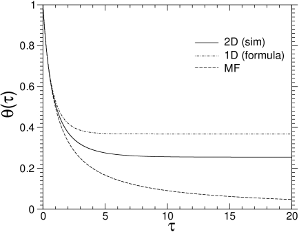
Figure 1: Comparative plot displaying the analytical $1D$ solution for the coverage, the $2D$ simulation result on a square lattice and the MF solution for the CR model.

Fig. 1 shows the coverage $\theta$ as a function of the dimensionless time for the CR model. For an initially full lattice, a comparative plot between the $1D$ solution, the MC result on the $2D$ square lattice and the simple MF approach is displayed. In the square lattice case, the mean coverage does not significantly change for times $\tau\approx 10$ and above, and its limiting value is found to be $0.2549$, about $30.7\%$ smaller than the $1D$ result $e^{-1}\approx 0.3679$. As expected, the higher connectivity of the $2D$ lattice ($z=4$, in contrast to $z=2$ for the $1D$ case) leads to an increased number of reactive events per occupied site, and the system gets closer to the empty state. As in the $1D$ case, the long-time decay to the final state appears to be well fitted by an exponential.

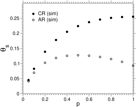
Figure 2: Comparative plot showing the $p$-dependence of the asymtotic coverage for the CR and the AR models on a $2D$ square lattice.

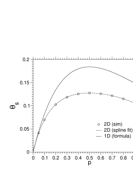
Figure 3: Nonmonotonic behavior of the final coverage as a function of the initial coverage $p$ in the AR case. The continuous line displays the $1D$ analytic result, while the dots correspond to simulation results on the $2D$ square lattice. The dot-dashed curve represents a spline fit of the MC results.

In the AR case, the simulation yields the exact value $\theta_{S}=0.0932$ for an initially full lattice, off by about $31.1\%$ from the exact value in $1D$. Fig. 2 shows the stationary coverage $\theta_{S}$ as a function of $p$ for both the CR and the AR. The dependence is monotonic for the CR, whereas a maximum at $p=0.5$ is observed in the AR case. As in the case of a Bethe lattice, this generic dependence on the initial coverage is likely to be robust in hypercubic lattices with arbitrary coordination number (cf. Fig. 3 for the AR case).

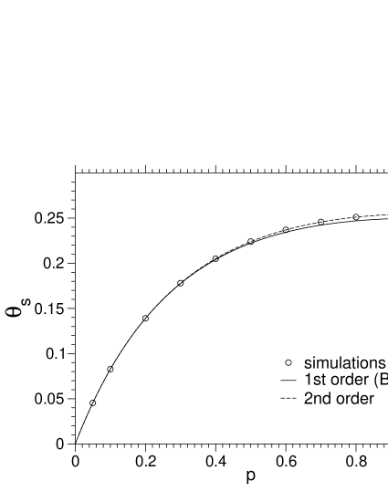
Figure 4: Exact simulation results for the CR vs. the first two orders of the shortest unshielded path approximation (the first order corresponds to a Bethe lattice). Note the good agreement of the second order results with the simulation over the whole $p$ range.

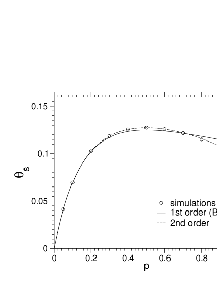
Figure 5: Exact simulation results for the AR vs. the first two orders of the shortest unshielded path approximation (the first order corresponds to a Bethe lattice). Note that the agreement of the approximate results with the simulation in the saturation region $p\approx 1$ is worse than in the CR case.

For $p=1$ and the CR ($\nu=1$), we get $\theta_{S}=1/4=0.25$ from Eq. (13), which is smaller than the simulation value by $19.2\%$ (cf. Fig. 4 and Table 1), whereas for $\nu=2$, the formula (13) yields $\theta_{S}=1/9=0.1111$, which is larger than the exact numerical value by $16.1\%$ (cf. Fig. 5 and Table 2). Thus, for a sufficiently large $p$, the first-order truncation (Bethe lattice solution) underestimates the asymptotic coverage in the CR case and overestimates it in the AR case.

On the other hand, for sufficiently low values of $p$ the approximation gets better in both cases. Thus, for $p=0.5$ the simulation value is larger than the approximated one by just $0.8\%$ for the CR (cf. Table 1). The fact that, for a given order of truncation, the accuracy increases monotonically with $p$ in the parametric region $p\ll 1$ corresponding to a dilute system is by no means surprising: in the dilute limit the $z=4$ Bethe lattice becomes a good approximation for the $2D$ square lattice, since “lattice animals” containing loops become rare.

III.2 Second-order approximation

For the second-order approximation, we take the whole set (10) as a starting point and make the approximations

$$Q_{\begin{picture}(15.0,10.0)\put(2.0,4.0){\circle*{4.0}}\put(8.0,4.0){\circle*{4.0}}\put(14.0,4.0){\circle*{4.0}} \put(7.0,0.0){\line(1,4){2.5}}\put(13.0,0.0){\line(1,4){2.5}} \end{picture}},Q_{\begin{picture}(15.0,15.0)\put(2.0,9.0){\circle*{4.0}}\put(8.0,9.0){\circle*{4.0}}\put(14.0,9.0){\circle*{4.0}} \put(7.0,5.0){\line(1,4){2.5}}\put(13.0,5.0){\line(1,4){2.5}} \put(14.0,1.0){\circle*{4.0}} \put(13.0,-3.0){\line(1,4){2.5}} \end{picture}},Q_{\begin{picture}(15.0,15.0)\put(2.0,9.0){\circle*{4.0}}\put(8.0,9.0){\circle*{4.0}} \put(7.0,5.0){\line(1,4){2.5}} \put(14.0,1.0){\circle*{4.0}} \put(13.0,-3.0){\line(1,4){2.5}} \end{picture}}\rightarrow Q_{\begin{picture}(10.0,10.0)\put(2.0,4.0){\circle*{4.0}} \put(8.0,4.0){\circle*{4.0}} \put(7.0,0.0){\line(1,4){2.5}} \end{picture}};\quad Q_{\begin{picture}(15.0,15.0)\put(2.0,9.0){\circle*{4.0}}\put(8.0,9.0){\circle*{4.0}}\put(14.0,9.0){\circle*{4.0}} \put(7.0,5.0){\line(1,4){2.5}}\put(13.0,5.0){\line(1,4){2.5}} \put(8.0,1.0){\circle*{4.0}} \put(7.0,-3.0){\line(1,4){2.5}} \end{picture}},Q_{\begin{picture}(15.0,15.0)\put(2.0,9.0){\circle*{4.0}}\put(8.0,9.0){\circle*{4.0}} \put(7.0,5.0){\line(1,4){2.5}} \put(8.0,1.0){\circle*{4.0}}\put(14.0,1.0){\circle*{4.0}} \put(7.0,-3.0){\line(1,4){2.5}}\put(13.0,-3.0){\line(1,4){2.5}} \end{picture}}\rightarrow Q_{\begin{picture}(10.0,15.0)\put(2.0,9.0){\circle*{4.0}}\put(8.0,9.0){\circle*{4.0}} \put(7.0,5.0){\line(1,4){2.5}} \put(8.0,1.0){\circle*{4.0}} \put(7.0,-3.0){\line(1,4){2.5}} \end{picture}};\quad Q_{\begin{picture}(10.0,15.0)\put(2.0,9.0){\circle*{4.0}}\put(8.0,9.0){\circle*{4.0}} \put(7.0,5.0){\line(1,4){2.5}} \put(2.0,1.0){\circle*{4.0}}\put(8.0,1.0){\circle*{4.0}} \put(1.0,-3.0){\line(1,4){2.5}}\put(7.0,-3.0){\line(1,4){2.5}} \end{picture}}\rightarrow Q_{\begin{picture}(15.0,15.0)\put(2.0,9.0){\circle*{4.0}}\put(8.0,9.0){\circle*{4.0}} \put(7.0,5.0){\line(1,4){2.5}} \put(2.0,1.0){\circle*{4.0}} \put(1.0,-3.0){\line(1,4){2.5}} \end{picture}},$$

thereby retaining all unshielded paths with lengths smaller than or equal to two lattice spacings. With this approximation we get from Eqs. (10)

$$\frac{d}{d\tau}\ln Q_{\begin{picture}(10.0,8.0)\put(4.0,2.0){\circle*{4.0}} \end{picture}} = -2\,\nu\,Q_{\begin{picture}(10.0,10.0)\put(2.0,4.0){\circle*{4.0}} \put(8.0,4.0){\circle*{4.0}} \put(7.0,0.0){\line(1,4){2.5}} \end{picture}},$$ (15a)

$$\frac{d}{d\tau}\ln Q_{\begin{picture}(10.0,10.0)\put(2.0,4.0){\circle*{4.0}} \put(8.0,4.0){\circle*{4.0}} \put(7.0,0.0){\line(1,4){2.5}} \end{picture}} = -1+\nu\,Q_{\begin{picture}(10.0,10.0)\put(2.0,4.0){\circle*{4.0}} \put(8.0,4.0){\circle*{4.0}} \put(7.0,0.0){\line(1,4){2.5}} \end{picture}}-2\nu\,Q_{\begin{picture}(10.0,15.0)\put(2.0,9.0){\circle*{4.0}}\put(8.0,9.0){\circle*{4.0}} \put(7.0,5.0){\line(1,4){2.5}} \put(8.0,1.0){\circle*{4.0}} \put(7.0,-3.0){\line(1,4){2.5}} \end{picture}},$$ (15b)

$$\frac{d}{d\tau}\ln Q_{\begin{picture}(10.0,15.0)\put(2.0,9.0){\circle*{4.0}}\put(8.0,9.0){\circle*{4.0}} \put(7.0,5.0){\line(1,4){2.5}} \put(8.0,1.0){\circle*{4.0}} \put(7.0,-3.0){\line(1,4){2.5}} \end{picture}} = -1-\nu\,Q_{\begin{picture}(15.0,15.0)\put(2.0,9.0){\circle*{4.0}}\put(8.0,9.0){\circle*{4.0}} \put(7.0,5.0){\line(1,4){2.5}} \put(2.0,1.0){\circle*{4.0}} \put(1.0,-3.0){\line(1,4){2.5}} \end{picture}},$$ (15c)

$$\frac{d}{d\tau}\ln Q_{\begin{picture}(15.0,15.0)\put(2.0,9.0){\circle*{4.0}}\put(8.0,9.0){\circle*{4.0}} \put(7.0,5.0){\line(1,4){2.5}} \put(2.0,1.0){\circle*{4.0}} \put(1.0,-3.0){\line(1,4){2.5}} \end{picture}} = -2+\nu\,Q_{\begin{picture}(10.0,10.0)\put(2.0,4.0){\circle*{4.0}} \put(8.0,4.0){\circle*{4.0}} \put(7.0,0.0){\line(1,4){2.5}} \end{picture}}-2\nu\,Q_{\begin{picture}(10.0,15.0)\put(2.0,9.0){\circle*{4.0}}\put(8.0,9.0){\circle*{4.0}} \put(7.0,5.0){\line(1,4){2.5}} \put(8.0,1.0){\circle*{4.0}} \put(7.0,-3.0){\line(1,4){2.5}} \end{picture}}+\nu\,Q_{\begin{picture}(15.0,15.0)\put(2.0,9.0){\circle*{4.0}}\put(8.0,9.0){\circle*{4.0}} \put(7.0,5.0){\line(1,4){2.5}} \put(2.0,1.0){\circle*{4.0}} \put(1.0,-3.0){\line(1,4){2.5}} \end{picture}}.$$ (15d)

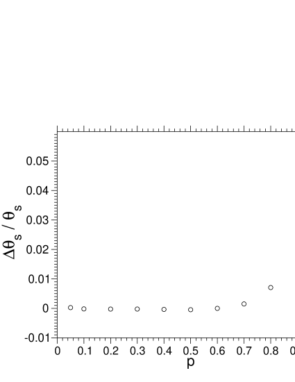
Figure 6: Relative error of $\theta_{S}$ as a function of $p$ in the second order approximation for the AR case.

An analytical solution for these equations does not seem possible, but they can be integrated numerically. The results for the stationary coverage are given in Tables 1 and 2. They are significantly better for the CR case; the deviation from the numerical result is maximal for $p=1$ and is about $-0.4\%$; its absolute value $|\Delta\theta_{S}/\theta_{S}|$ diminishes monotonically with decreasing $p$. In contrast, the maximal deviation for $p=1$ in the AR case makes about $5.3\%$ (cf. Fig. 6).

Better approximations can be obtained at higher orders, but the number of conditional probabilities to be taken into account grows dramatically. It then becomes necessary to automate the generation of the hierarchical equations. For instance, to third order one has 24 different probabilities and to fourth order, 766 Nord .

Nevertheless, the approximate conditional probabilities obtained from the second-order hierarchy (15) are already in good agreement with exact simulation results, both at the level of the stationary coverage and at the level of the time evolution (data not shown). Interestingly, the dynamics turns out to be qualitatively different depending on the value of $\nu$. In the CR case the inequality $Q_{\begin{picture}(10.0,8.0)\put(4.0,2.0){\circle*{4.0}} \end{picture}}>Q_{\begin{picture}(10.0,10.0)\put(2.0,4.0){\circle*{4.0}} \put(8.0,4.0){\circle*{4.0}} \put(7.0,0.0){\line(1,4){2.5}} \end{picture}}$ holds for all times, while in the AR case this is only true provided that the initial coverage is sufficiently low, i.e. for $p<1/2$. This behavior is observed in Fig. 7, which also displays the time evolution of the other conditional probabilities (for typographical reasons, the symbols $Q_{1},Q_{2},Q_{3}$ and ${Q_{3}}^{{}^{\prime}}$ used in the legend represent respectively the quantities $Q_{\begin{picture}(10.0,8.0)\put(4.0,2.0){\circle*{4.0}} \end{picture}},Q_{\begin{picture}(10.0,10.0)\put(2.0,4.0){\circle*{4.0}} \put(8.0,4.0){\circle*{4.0}} \put(7.0,0.0){\line(1,4){2.5}} \end{picture}},Q_{\begin{picture}(10.0,15.0)\put(2.0,9.0){\circle*{4.0}}\put(8.0,9.0){\circle*{4.0}} \put(7.0,5.0){\line(1,4){2.5}} \put(8.0,1.0){\circle*{4.0}} \put(7.0,-3.0){\line(1,4){2.5}} \end{picture}}$ and $Q_{\begin{picture}(15.0,15.0)\put(2.0,9.0){\circle*{4.0}}\put(8.0,9.0){\circle*{4.0}} \put(7.0,5.0){\line(1,4){2.5}} \put(2.0,1.0){\circle*{4.0}} \put(1.0,-3.0){\line(1,4){2.5}} \end{picture}}$).

In contrast, above $p=1/2$ the AR system displays a crossover between a short time regime for which $Q_{\begin{picture}(10.0,8.0)\put(4.0,2.0){\circle*{4.0}} \end{picture}}<Q_{\begin{picture}(10.0,10.0)\put(2.0,4.0){\circle*{4.0}} \put(8.0,4.0){\circle*{4.0}} \put(7.0,0.0){\line(1,4){2.5}} \end{picture}}$ and a long time regime with $Q_{\begin{picture}(10.0,8.0)\put(4.0,2.0){\circle*{4.0}} \end{picture}}>Q_{\begin{picture}(10.0,10.0)\put(2.0,4.0){\circle*{4.0}} \put(8.0,4.0){\circle*{4.0}} \put(7.0,0.0){\line(1,4){2.5}} \end{picture}}$ beyond a $p$-dependent crossover time (see Fig. 8 ). I.e., for short times the probability to find a site occupied given that its neighbor is occupied is larger than for a randomly chosen site with no previous information on the state of the neighbor site, whereas for long times the opposite is true. Remarkably enough, the qualitative behavior of both reaction schemes appears to be universal, in the sense that it remains the same in Bethe lattices of arbitrary coordination number (cf. Eqs. 5).

As far as higher order conditional probabilities are concerned, the inequality $Q_{\begin{picture}(10.0,8.0)\put(4.0,2.0){\circle*{4.0}} \end{picture}}>Q_{\begin{picture}(10.0,10.0)\put(2.0,4.0){\circle*{4.0}} \put(8.0,4.0){\circle*{4.0}} \put(7.0,0.0){\line(1,4){2.5}} \end{picture}}>Q_{\begin{picture}(10.0,15.0)\put(2.0,9.0){\circle*{4.0}}\put(8.0,9.0){\circle*{4.0}} \put(7.0,5.0){\line(1,4){2.5}} \put(8.0,1.0){\circle*{4.0}} \put(7.0,-3.0){\line(1,4){2.5}} \end{picture}}>Q_{\begin{picture}(15.0,15.0)\put(2.0,9.0){\circle*{4.0}}\put(8.0,9.0){\circle*{4.0}} \put(7.0,5.0){\line(1,4){2.5}} \put(2.0,1.0){\circle*{4.0}} \put(1.0,-3.0){\line(1,4){2.5}} \end{picture}}$ holds at all times both in the CR case and in the dilute AR case with $p<1/2$ (cf. Fig. 7 ). However, for sufficiently short times we again observe a departure from this behavior at higher $p$ in the AR case. In fact, all three conditional probabilities $Q_{\begin{picture}(10.0,8.0)\put(4.0,2.0){\circle*{4.0}} \end{picture}},Q_{\begin{picture}(10.0,10.0)\put(2.0,4.0){\circle*{4.0}} \put(8.0,4.0){\circle*{4.0}} \put(7.0,0.0){\line(1,4){2.5}} \end{picture}},Q_{\begin{picture}(10.0,15.0)\put(2.0,9.0){\circle*{4.0}}\put(8.0,9.0){\circle*{4.0}} \put(7.0,5.0){\line(1,4){2.5}} \put(8.0,1.0){\circle*{4.0}} \put(7.0,-3.0){\line(1,4){2.5}} \end{picture}}$ become larger than $Q_{\begin{picture}(10.0,8.0)\put(4.0,2.0){\circle*{4.0}} \end{picture}}$ for a sufficiently large $p$ (cf. Fig. 8 ). In this regime, the detailed behavior of the above $Q$ probabilities with respect to each other is rather complex and shall not be further discussed here.

In order to interpret some of the above results, let us first characterize the occupation of a given site $i$ by an occupation number $n_{i}$ (equal to one if the site is occupied and zero otherwise). The fluctuation $\delta n_{i}$ is defined as the deviation from the average occupation in a given statistical realization, i.e. $\delta n_{i}=n_{i}-\langle n_{i}\rangle$. A special kind of two-site fluctuation correlation is then $f_{m}\equiv\langle\,\delta n_{i}\,\delta n_{i+m}\rangle$, where $i$ and $i+m$ are two sites separated by $m$ bonds along a $1D$ path. By definition, $f_{m}$ is translationally invariant and depends only on the distance $m$.

The behavior of the conditional probabilities in our hierarchy is given by the cluster probabilities $P$. In turn, the latter are related to the fluctuation correlations, which measure the reaction-induced ordering in the system. E.g., the sign of the difference $Q_{\begin{picture}(10.0,8.0)\put(4.0,2.0){\circle*{4.0}} \end{picture}}-Q_{\begin{picture}(10.0,10.0)\put(2.0,4.0){\circle*{4.0}} \put(8.0,4.0){\circle*{4.0}} \put(7.0,0.0){\line(1,4){2.5}} \end{picture}}$ is the same as the sign of the nearest neighbour two-site fluctuation correlation $f_{1}=P_{\begin{picture}(10.0,10.0)\put(2.0,4.0){\circle*{4.0}}\put(8.0,4.0){\circle*{4.0}} \end{picture}}-P_{\begin{picture}(10.0,8.0)\put(4.0,2.0){\circle*{4.0}} \end{picture}}^{\,\,2}=(Q_{\begin{picture}(10.0,10.0)\put(2.0,4.0){\circle*{4.0}} \put(8.0,4.0){\circle*{4.0}} \put(7.0,0.0){\line(1,4){2.5}} \end{picture}}-Q_{\begin{picture}(10.0,8.0)\put(4.0,2.0){\circle*{4.0}} \end{picture}})\,Q_{\begin{picture}(10.0,8.0)\put(4.0,2.0){\circle*{4.0}} \end{picture}}$. In all cases $f_{1}<0$ as $\tau\to\infty$, since two-particle clusters disappear. In Fig. 9 MC computations for the dynamical behavior of the two-site correlations $f_{1},f_{2},f_{3}$ and the three site correlation $h=\langle\delta n_{i}\,\delta n_{i+1}\,\delta n_{i+2}\rangle$ in the dilute AR case ($p<\frac{1}{2}$) are shown. As in the CR case, one has $f_{1}<0$ for all times, i.e $P_{\begin{picture}(10.0,10.0)\put(2.0,4.0){\circle*{4.0}}\put(8.0,4.0){\circle*{4.0}} \end{picture}}>P_{\begin{picture}(10.0,8.0)\put(4.0,2.0){\circle*{4.0}} \end{picture}}^{\,\,2}$. However, as soon as $p>1/2$, one has $f_{1}>0$ for sufficiently short times (see Fig 10). In other words, the probability to find a pair of neighboring sites simultaneously occupied is higher than if both sites are chosen at random. Most probably, the reason is that for short times the typical size of particle islands is still relatively large, and so is the value of $P_{\begin{picture}(10.0,10.0)\put(2.0,4.0){\circle*{4.0}}\put(8.0,4.0){\circle*{4.0}} \end{picture}}$ ; however, the reaction-induced growth of empty site clusters takes place at a higher rate than in the CR case. Thus, the probability that one finds an empty site beyond a certain correlation length from a given particle is comparatively high, thereby decreasing the value of $P_{\begin{picture}(10.0,8.0)\put(4.0,2.0){\circle*{4.0}} \end{picture}}^{\,\,2}$.

As for the behavior of $f_{2}$,$f_{3}$ and $h$, both schemes again display very similar qualitative features in the low-$p$ regime. The numerical plots in Fig. 9 suggest that $f_{2}>0$ and $f_{3}<0$ for all times (for very short times, however, our precision does not allow to determine the sign of the correlation functions). In any case, this holds for the stationary values of these quantities as $\tau\to\infty$. In terms of conditional probabilities, this means that $Q_{\begin{picture}(15.0,10.0)\put(2.0,4.0){\circle*{4.0}}\put(14.0,4.0){\circle*{4.0}} \put(6.0,2.0){-} \put(13.0,0.0){\line(1,4){2.5}} \end{picture}}>Q_{\begin{picture}(10.0,8.0)\put(4.0,2.0){\circle*{4.0}} \end{picture}}$ and $Q_{\begin{picture}(22.0,10.0)\put(2.0,4.0){\circle*{4.0}}\put(20.0,4.0){\circle*{4.0}} \put(6.0,2.0){- -} \put(19.0,0.0){\line(1,4){2.5}} \end{picture}}<Q_{\begin{picture}(10.0,8.0)\put(4.0,2.0){\circle*{4.0}} \end{picture}}$, where “-” denotes a site in an unspecified state. Notice also that the absolute value of the three-site correlation $|h|$ becomes significantly larger than $|f_{3}|$. Moreover, for yet smaller values of the initial coverage $|h|$ may get larger than $|f_{2}|$. This suggests that any expansion of the cluster probabilities retaining only two-site correlation functions fails to describe the behavior, since long-range correlations propagate throughout the system in the course of reaction. As a matter of fact, in the $1D$ case such an expansion leads to a zero stationary coverage to any order of the distance between sites thes .

At higher values of $p$, the behavior is again modified in the AR case. The functions $f_{2}$ and $f_{3}$ change sign, and the above inequalities for the conditional probabilities change their direction. In contrast, $h$ keeps its positive sign but decreases strongly.

The analysis presented in this subsection suggests that the nature of the spatial self-ordering as a function of the initial condition is rather complex (specially in the AR case) and remains to be fully characterized.

IV Conclusions and outlook

Using the analogy with RSA problems, we have used the method of conditional probabilities to compute estimates for the lattice coverage in the framework of a unifying description for two different types of irreversible binary reactions, i.e. coalescence and annihilation. More traditional methods based on a spatial cut-off of fluctuations fail here, since the latter are propagated by the reactions over the whole system size. In contrast, the method of conditional probabilities is exact in $1D$ and branching media such as Bethe lattices, which can be used as a starting point for density expansions in other regular lattices Evans3 (in the dilute limit, the Bethe lattice approximation should be good, since clusters with loops are rare). A further advantage of the method is that it provides a reasonable approximation for the “exact” simulation results beyond the dilute limit, thereby allowing to obtain a fairly good estimate in the vicinity of $p=1$ (corresponding to the usual initial condition in RSA problems). Remarkably, the expansion for the CR model in this regime provides a better approximation than for the AR model.

The approach used in the present paper can also be applied to mixed systems combining both coalescence and annihilation steps as well as to more complex kinds of initial condition cadil . The correspondence between such models and RSA problems may prove useful in the context of pre-patterning of the substrate as a tool to improve self-assembly in certain systems.

We have also seen that our model yields good results for the fluctuation-induced dynamical behavior of the system. The main conclusion is that the subsequent dynamics of the spatial distribution is very sensitive with respect to the details of the initial condition, specially in the AR case, where several types of crossovers for the correlation functions have been identified.

Possible extensions of our work include a more complete characterization of the transient behavior of the spatial distribution for the reactant species (and not only for the special kind of correlation functions considered here) as well as its dependence on the initial condition. However, exact decimation at any scale is in principle only possible in one dimension bonnier and probably also on Bethe lattices, but the analogous problem on a lattice with loops still requires the use of approximate techniques.

In the above context, it is also of interest to compare the properties of such systems with those of their diffusion-controlled counterparts. This work could then be further extended to other systems such as the two-species annihilation $A+B\rightarrow S+S$. This reaction is known to induce reactant segregation at low dimensions and has been widely investigated in the diffusion-controlled case Ovch ; Touss ; Kuz ; Bram ; Schn ; linden ; sancho , but its version with immobile reactants Priv has not received much attention yet. In particular, it would be interesting to see whether a shielding property can also be derived in this case, at least for a specific kind of initial conditions.

Figure 7: Time evolution of the conditional probabilities obtained from Eqs. (15) for the AR case in the dilute regime ($p=0.25$).

Figure 8: Time evolution of the conditional probabilities obtained from Eqs. (15) for the AR case in the saturation regime ($p=1$). The legend uses the same notation as in Fig. 7.

Figure 9: Dynamical behavior of the first three two-site fluctuation correlation functions and the three-site correlation function $h$ in the dilute AR case ($p=0.25$). For this computation we have performed simulations over 5000 realizations on a $200\times 200$ lattice.

Figure 10: Dynamical behavior of the first three two-site fluctuation correlation functions and the three-site correlation function $h$ in the AR case with an initially full lattice ($p=1$). The simulation parameters are the same as in Fig. 9.

$p$	MC Simulation	truncation (1st. ord.)	truncation (2nd. ord.)
0.05	0.04535379	0.04535147	0.04535233
0.1	0.08265606	0.08264463	0.08265592
0.2	0.1390146	0.1388889	0.1390138
0.3	0.1779778	0.1775148	0.1779583
0.4	0.2050887	0.2040816	0.2050757
0.5	0.2239603	0.2222222	0.2223642
0.6	0.2369787	0.2343750	0.2369514
0.7	0.2456631	0.2422145	0.2456311
0.8	0.2510806	0.2469136	0.2510572
0.9	0.2540033	0.2493075	0.2539584
1	0.2549411	0.2500000	0.2548402

Table 1: A comparison between the values of $\theta_{S}$ obtained from MC simulations and the approximated values obtained by truncation of the hierarchy for the CR model.

$p$	MC Simulation	truncation (1st. ord.)	truncation (2nd. ord.)
0.05	0.04131765	0.04132231	0.04132796
0.1	0.06952005	0.06944444	0.06950689
0.2	0.1025630	0.1020408	0.1025378
0.3	0.1185036	0.1171875	0.1184757
0.4	0.1255734	0.1234568	0.1255286
0.5	0.1274785	0.1250000	0.1274201
0.6	0.1259282	0.1239669	0.1259275
0.7	0.1217432	0.1215278	0.1219250
0.8	0.1150304	0.1183432	0.1158427
0.9	0.1057193	0.1147959	0.1078826
1	0.09318323	0.1111111	0.09812664

Table 2: A comparison between the values of $\theta_{S}$ obtained from MC simulations and the approximated values obtained by truncation of the hierarchy for the AR model.

References

- (1) N. G. van Kampen, Stochastic processes in Chemistry and Physics (North Holland, Amsterdam, 1983).
- (2) C. W. Gardiner, Handbook of Stochastic Methods (Springer, Berlin, 1983).
- (3) G. Nicolis and I. Prigogine Self-organisation in Non-equilibrium Systems (Wiley, New York, 1977).
- (4) Yu. Suchorski, J. Beben, and R. Imbihl, Surf. Sci. 405, L477 (1998).
- (5) Yu. Suchorski, J. Beben, and R. Imbihl, Prog. Surf. Sci. 59, 343 (1998).
- (6) D. ben-Avraham and S. Havlin, Diffusion and Reactions in Fractals and Disordered Systems (Cambridge University Press, Cambridge, 2000).
- (7) D. ben-Avraham, M. Burschka, and C. R. Doering, J. Stat. Phys. 60, 695 (1990).
- (8) J. L. Spouge, Phys. Rev. Lett. 60, 871 (1988).
- (9) E. Abad, H. L. Frisch, and G. Nicolis, J. Stat. Phys. 99, 1397 (2000).
- (10) D. C. Torney and H. M. McConnell, J. Phys. Chem. 87, 1941 (1983).
- (11) A. A. Lushnikov, Phys. Lett. A 120, 135 (1987).
- (12) J. G. Amar and F. Family, Phys. Rev. A 41, 3258 (1990).
- (13) G. M. Schütz, J. Phys. A 28, 3405 (1995).
- (14) M. D. Grynberg and R. Stinchcombe, Phys. Rev. Lett. 76, 851 (1996).
- (15) F. Leyvraz and S. Redner, Phys. Rev. A 36, 4033 (1987).
- (16) A. Provata, H. Takayasu, and M. Takayasu, Europhys. Lett.33, 99 (1996).
- (17) R. Kopelman, Science 241, 1620 (1988).
- (18) P. W. Klymko and R. Kopelman, J. Phys. Chem. 87, 4565 (1983).
- (19) R. Kroon and R. Sprik in Nonequilibrium Statistical Mechanics in One Dimension ed. by V. Privman (Cambridge Univ. Press, Cambridge, 1997).
- (20) Z. Rácz, Phys. Rev. Lett. 55, 1707 (1985).
- (21) J. L. Jackson and E. W. Montroll, J. Chem. Phys. 28, 1101 (1958).
- (22) E. R. Cohen and H. Reiss, J. Chem. Phys. 38, 680 (1963).
- (23) M. C. Bartelt and V. Privman, Int. J. Mod. Phys. B 5, 2883 (1991).
- (24) J. W. Evans, Rev. Mod. Phys. 65, 1281 (1993).
- (25) M. J. de Oliveira, T. Tomé, and R. Dickman, Phys. Rev. A 46, 6294 (1992).
- (26) J. B. Keller, J. Chem. Phys. 38, 325 (1963).
- (27) L. G. Mityushin, Prob. Peredachi Inf. 9, 81 (1973).
- (28) Y. Fan and J. K. Percus, Phys. Rev. A 44, 5099 (1991).
- (29) F. Baras, F. Vikas, and G. Nicolis, Phys. Rev. E 60, 3797 (1999).
- (30) E. Abad, P. Grosfils, and G. Nicolis, Phys. Rev. E 63, 041102 (2001).
- (31) J. W. Evans, J. Math. Phys. 25, 2527 (1984).
- (32) S. N. Majumdar and V. Privman, J. Phys. A 26, L743 (1993).
- (33) R. S. Nord and J. W. Evans, J. Chem. Phys. 82, 2795 (1985).
- (34) K. J. Vette, T. W. Orent, D. K. Hoffman, and R. S. Hansen, J. Chem. Phys. 60, 4584 (1974).
- (35) M. Malek-Mansour and J. Houard, Phys. Lett. 70A, 366 (1979).
- (36) E. Abad, A. Provata, and G. Nicolis, Europhys. Lett. 61, 586 (2003).
- (37) E. Abad, Ph.D. Thesis (Université Libre de Bruxelles, Brussels, 2003)
- (38) P. J. Flory, J. Am. Chem. Soc. 61, 1518 (1939).
- (39) V. M. Kenkre and H. M. Van Horn, Phys. Rev. A 23, 3200 (1981).
- (40) A. M. R. Cadilhe and V. Privman, Modern Phys. Lett. B 18, 207 (2004).
- (41) B. Bonnier, R. Brown, and E. Pommiers, J. Phys. A 28, 5165 (1995).
- (42) A. A. Ovchinnikov and Y. B. Zeldovich, Chem. Phys. 28, 215 (1978).
- (43) D. Toussaint and F. Wilczek, J. Chem. Phys. 78, 2642 (1983).
- (44) V. Kuzovkov and E. Kotomin, Rep. Prog. Phys. 51, 1479 (1988).
- (45) M. Bramson and J. L. Lebowitz, Phys. Rev. Lett. 61, 2397 (1988)
- (46) H. Schnörer, V. Kuzovkov, and A. Blumen, Phys. Rev. Lett. 63, 805 (1990).
- (47) K. Lindenberg, B. J. West, and R. Kopelman, Phys. Rev. A 42, 890 (1990).
- (48) J. M. Sancho, A. H. Romero, K. Lindenberg, F. Sagués, R. Reigada, and A. M. Lacasta, J. Phys. Chem. 100, 19066 (1996).