Optical conductivity of the one-dimensional dimerized Hubbard model at quarter filling

Abstract

We investigate the optical conductivity in the Mott insulating phase of the one-dimensional extended Hubbard model with alternating hopping terms (dimerization) at quarter band filling. Optical spectra are calculated for the various parameter regimes using the dynamical density-matrix renormalization group method. The study of limiting cases allows us to explain the various structures found numerically in the optical conductivity of this model. Our calculations show that the dimerization and the nearest-neighbor repulsion determine the main features of the spectrum. The on-site repulsion plays only a secondary role. We discuss the consequences of our results for the theory of the optical conductivity in the Bechgaard salts.

1 Introduction

The electronic properties of quasi-one-dimensional charge-transfer salts have been intensively investigated in recent years Farges ; Ishiguro ; Bourbonnais . An important example of such compounds is the family of Bechgaard salts $({\rm TM})_{2}X$, where TM is the organic molecule TMTSF (tetramethyltetraselenafulvalene) or TMTTF (tetramethyltetrathiafulvalene), and X denotes an anion such as ${\rm ClO}^{-}_{4}$, ${\rm PF}_{6}^{-}$, ${\rm Br}^{-}$, etc. These materials have highly anisotropic structures and properties. Therefore, it is believed that above an energy scale of a few meV their electronic properties can be described in first approximation by one-dimensional models.

The one-dimensional Hubbard model with alternating hopping integrals (dimerization) and a quarter-filled band has been proposed to describe various properties of the Bechgaard salts pen94 ; mil95 ; fav96 ; nis00 ; shi01 ; tsu01 , in particular their unusual optical spectrum ped94 ; dre96 ; ves98 ; sch98 ; ves00 . In this model the formation of a Mott insulating ground state is due to the interplay of the Coulomb interaction between electrons and the lattice dimerization. However, the relevance of this approach for Bechgaard salts has remained controversial. Although we know the generic features of the low-energy optical spectrum in one-dimensional Mott insulators jec00 ; con01 ; gia91 , the optical conductivity of the quarter-filled Hubbard model with dimerization has not been determined accurately yet. Thus, no direct comparison with the experimental spectrum observed in Bechgaard salts has been possible.

The recent development of the dynamical density matrix renormalization-group (DDMRG) method jec00 ; jec02 allows us to calculate the dynamical properties of low dimensional correlated electron systems with an accuracy comparable to exact diagonalizations but for much larger system sizes. Here, we apply the DDMRG method to the calculation of the optical conductivity in the quarter-filled dimerized Hubbard model. The model and method are briefly introduced in the next section. Then, we present our results in Sec. 3. Finally, we discuss the consequences of our results for the theory of the Bechgaard salts in Sec. 4.

2 Model and Method

The one-dimensional extended and dimerized Hubbard model is defined by the Hamiltonian

$$\hat{H} = -t_{1}\sum_{{\rm odd}\ l;\sigma}\left(\hat{c}_{l,\sigma}^{{\dagger}}\hat{c}_{l+1,\sigma}^{\phantom{{\dagger}}}+\hat{c}_{l+1,\sigma}^{{\dagger}}\hat{c}_{l,\sigma}^{\phantom{{\dagger}}}\right)$$

$$-t_{2}\sum_{{\rm even}\ l;\sigma}\left(\hat{c}_{l,\sigma}^{{\dagger}}\hat{c}_{l+1,\sigma}^{\phantom{{\dagger}}}+\hat{c}_{l+1,\sigma}^{{\dagger}}\hat{c}_{l,\sigma}^{\phantom{{\dagger}}}\right)$$

$$+U\sum_{l}\hat{n}_{l,\uparrow}\hat{n}_{l,\downarrow}+V\sum_{l}(\hat{n}_{l}-\rho)(\hat{n}_{l+1}-\rho)\;.$$

It describes fermions with spin $\sigma=\uparrow,\downarrow$ which can hop between neighboring sites representing the highest occupied molecular orbital (HOMO) of each TM molecule. There are three electrons in the HOMOs of each pair $({\rm TM})_{2}$, so that the band made of the HOMOs is three-quarter filled in terms of electrons or quarter filled in terms of holes. We use the hole representation and keep the number of particles $N$ such that we have a density $\rho=N/L=1/2$ for an even number of lattice sites $L$. The operator $\hat{c}^{+}_{l,\sigma}$ ($\hat{c}_{l,\sigma}$) creates (annihilates) a hole with spin $\sigma$ at site $l$. The hole density operator is $\hat{n}_{l,\sigma}=\hat{c}^{+}_{l,\sigma}\hat{c}_{l,\sigma}$ and $\hat{n}_{l}=\hat{n}_{l,\uparrow}+\hat{n}_{l,\downarrow}$ is the total number of holes at site $l$. The hopping integrals $t_{1}\geq t_{2}\geq 0$ give rise to a single-particle dispersion

$$\epsilon(k)=\pm\sqrt{\Delta^{2}\sin^{2}(k)+4t^{2}\cos^{2}(k)}$$ (2)

with a total band width $4t=2t_{1}+2t_{2}$ and a (dimerization) gap $2\Delta=2(t_{1}-t_{2})$. The Coulomb repulsion is mimicked by a local Hubbard interaction $U$, and a nearest-neighbor interaction $V$. The physically relevant parameter regime for Bechgaard salts is $U>2V\geq 0$. In Table 1, we show some values of the model parameters $t_{1},t_{2},U$, and $V$ which have been proposed mil95 ; fav96 ; nis00 ; duc86 to describe various (TM)₂X salts.

We use open boundary conditions since density matrix renormalization group (DMRG) algorithms are most efficient for this type of boundary steve ; dmrgbook . In open chains it is important to use the correct form of the (non-local) Coulomb interaction between electrons in the Hamiltonian (2). Neglecting the average density (i.e., setting $\rho=0$ in Eq. 2) results in complicated edge effects in the excitation spectrum such as the existence of low-energy excitations localized at the chain ends.

Two mechanisms can induce an insulating ground state in this model at quarter filling shi01 ; tsu01 . First, the Umklapp scattering in an effectively half-filled band [$-2t\leq\epsilon(k)\leq-\Delta$] due to the dimerization can lead to a Mott insulating state accompanied by a $4k_{F}$ bond order wave (BOW), where $k_{F}=\pi\rho/2=\pi/4$ is the Fermi vector. Second, for large enough parameters $U$ and $V$ the Umklapp scattering in the quarter-filled band [$-2t\leq\epsilon(k)\leq 2t$, neglecting the dimerization gap $2\Delta$] can drive the ground state into an insulating phase with a spontaneously broken symmetry: a $4k_{F}$ charge density wave (CDW) shi01 ; hir84 ; mil93 . In the family of Bechgaard salts, TMTSF compounds are believed to be realizations of one-dimensional Mott insulators con01 while TMTTF compounds are considered to be charge ordered tsu01 like in a CDW state. For realistic parameters (see Table 1), however, the system described by the Hamiltonian (2) is a Mott insulator shi01 . Therefore, we will investigate the optical conductivity in the Mott insulating phase only. Since we use open boundary conditions, we observe $2k_{F}$-BOW and $2k_{F}$- and $4k_{F}$-CDW fluctuations induced by the chain ends (Friedel charge oscillations) in the ground state. For all the parameters $U,V,t_{1},t_{2}$ discussed in this work, however, the ground state has no long-range order or broken symmetry but the $4k_{F}$-BOW induced by the alternating hopping terms $t_{1}\neq t_{2}$.

Table 1: Model parameters (in meV) for various Bechgaard salts from Refs. mil95 ; fav96 ; nis00 ; duc86 .

		$t_{1}$	$t_{2}$	$U$	$V$
(TMTSF)2PF6	(Ref. fav96 )	250	225	1250	0
(TMTSF)2ClO4	(Ref. nis00 )	290	260	1450	210
(TMTTF)2PF6	(Refs. mil95 ; duc86 )	135	95	945	380

To determine the ground state properties and to obtain some information about excited states of the Hamiltonian (2) we use a standard DMRG technique steve ; dmrgbook . For instance, the Mott gap (also called single-particle charge gap or charge transfer gap)

$$E_{c}=E_{0}(N+1)+E_{0}(N-1)-2E_{0}(N)$$ (3)

can be calculated from the ground state energies $E_{0}(N_{h})$ for $N_{h}$ holes in the system pen94 ; nis00 .

The linear optical absorption is proportional to the real part $\sigma_{1}(\omega)$ of the optical conductivity, which is related to the imaginary part of the current-current correlation function by

$$\sigma_{1}(\omega>0)=\frac{-1}{L\omega}{\rm Im}\ \langle\psi_{0}|\hat{J}\frac{1}{E_{0}+\omega+i\eta-\hat{H}}\hat{J}|\psi_{0}\rangle\;.$$ (4)

Here, $|\psi_{0}\rangle$ is the ground state of the Hamiltonian $\hat{H}$, $E_{0}$ is the ground state energy, and $\eta\rightarrow 0^{+}$. Assuming that the sites are equidistant, the current operator $\hat{J}$ is

$$\hat{J} = -{\rm i}t_{1}\sum_{{\rm odd}\ l;\sigma}\left(\hat{c}_{l,\sigma}^{{\dagger}}\hat{c}_{l+1,\sigma}^{\phantom{{\dagger}}}-\hat{c}_{l+1,\sigma}^{{\dagger}}\hat{c}_{l,\sigma}^{\phantom{{\dagger}}}\right)$$ (5)

$$-{\rm i}t_{2}\sum_{{\rm even}\ l;\sigma}\left(\hat{c}_{l,\sigma}^{{\dagger}}\hat{c}_{l+1,\sigma}^{\phantom{{\dagger}}}-\hat{c}_{l+1,\sigma}^{{\dagger}}\hat{c}_{l,\sigma}^{\phantom{{\dagger}}}\right)\ .$$

With these definitions the optical conductivity $\sigma_{1}(\omega)$ is given in units of $e^{2}a/\hbar$, where $2a$ is the lattice constant and $e$ the charge of a hole. The frequency $\omega$ is given in units of $t/\hbar$.

In an open chain the optical conductivity is also related to the imaginary part of the dipole-dipole correlation function

$$\sigma_{1}(\omega)=\frac{-\omega}{L}{\rm Im}\ \langle\psi_{0}|\hat{D}\frac{1}{E_{0}+\omega+i\eta-\hat{H}}\hat{D}|\psi_{0}\rangle\;,$$ (6)

where the dipole operator is

$$\hat{D}=\sum_{l=1}^{L}l\left(\hat{n}_{l}-\rho\right)=\sum_{l=1}^{L}\left(l-\frac{L+1}{2}\right)\hat{n}_{l}.$$ (7)

One can apply the DDMRG method jec02 to chains of finite size $L$ to compute the optical conductivity $\sigma_{1}(\omega)$ with a finite broadening $\eta>0$. Thus, DDMRG yields the convolution of $\sigma_{1}(\omega)$ with a Lorentzian of width $\eta$ or the quantity defined by Eq. 4 or Eq. 6 for a finite $\eta$ (see Ref. jec02 for more details and the advantages of the various approaches). The properties of the optical spectrum in the thermodynamic limit $L\rightarrow\infty$ can be determined using a finite-size-scaling analysis jec02 with an appropriate broadening

$$\eta(L)\sim 1/L.$$ (8)

This approach has already been successfully used to study the optical properties of simple one-dimensional Mott insulators (i.e, in the extended Hubbard model at half filling) jec00 ; ess01 ; jec03 . In particular, a quantitative description has been achieved RIXS for the experimental low-energy optical conductivity spectrum in the quasi-one-dimensional compound SrCuO₂.

Often one can use deconvolution techniques to compute a smooth spectrum without broadening from the numerical DDMRG data for finite $\eta$ and finite system size geb04 ; uhrig . In this work we use a standard linear regularization method for the inverse problem numrep to deconvolve DDMRG spectra. The deconvolution usually yields a very accurate description of the spectrum in the thermodynamic limit if it does not possess any sharp feature (i.e., on a scale smaller than the broadening $\eta$ used in the DDMRG calculation). Therefore, the broadening $\eta$ used in the DDMRG calculation sets the resolution of a spectrum obtained through a deconvolution.

An extension of the DDMRG method jec02 can be used to compute the excited states of the Hamiltonian which contribute to the optical spectrum (4). We have used this method to determine the optical gap (i.e., the excitation energy $\omega_{1}$ of the lowest eigenstate $|\psi_{1}\rangle$ with a finite matrix element $\langle\psi_{1}|\hat{J}|\psi_{0}\rangle$) in finite chains more accurately.

Up to $m=320$ density-matrix eigenstates have been kept per block in DDMRG calculations and up to $m=768$ in ground state DMRG calculations. Truncation errors are negligible for all results presented here. Thus, the accuracy of our calculations is mostly limited by the finite broadening or resolution $\eta\sim 1/L$ imposed by finite system lengths.

3 Results

In the absence of the non-local electron-electron interaction ($V=0$), the properties of the model (2) depend on the parameters $U$ and $\Delta$ only. (The average hopping term $t$ just fixes the energy scale.) First, we will investigate three limiting cases pen94 for which the main features in the optical conductivity $\sigma_{1}(\omega)$ can be easily understood: (i) the large-dimerization limit $t_{2}\ll t_{1}(\Rightarrow\Delta\approx 2t)$, $U\leq 4t_{1}$, (ii) the strong-coupling limit $U\gg t_{1}>t_{2}$, and (iii) the weak-coupling limit $U\ll t_{2}<t_{1}$. Then we will discuss how the optical spectrum changes when the parameters $U$ and $\Delta$ are varied between the limiting cases. Finally, we will consider the effects of the nearest-neighbor repulsion $V$.

3.1 Large Dimerization

In the dimer limit $\Delta=2t$ ($t_{2}/t_{1}\rightarrow 0$) the system is made of independent dimers (i.e., pairs of nearest-neighbor sites) pen94 . The system eigenstates are products of the dimer eigenstates (i.e., the eigenstates of a two-site Hubbard model). In the ground state at quarter filling each dimer is occupied by exactly one hole, which is localized on that dimer. The current operator (5) does not couple the dimers. Therefore, only intra-dimer excitations can contribute to the optical conductivity. (They correspond to transitions from the bonding orbital to the anti-bonding orbital of the dimer in the limit $U=0$.) It can be shown that $\sigma_{1}(\omega)$ consists of a single Dirac $\delta$-peak at $\omega=2t_{1}=4t=2\Delta$ for any $U\geq 0$. Note, that moving one hole from a dimer to another one (inter-dimer excitations) yields eigenstates of the system with an excitation energy which can be lower than $2\Delta$ and thus the Mott gap $E_{c}$ is lower than the optical gap $\omega_{1}=2\Delta$ in that special case. (For instance, $E_{c}$ vanishes as $U$ goes to zero but $\omega_{1}=2\Delta>0$.)

Figure 1: Optical conductivity $\sigma_{1}(\omega)$ in the large-dimerization limit ($\Delta=1.64t$) for a strong effective coupling ($U=3.64t\approx 20t_{2}$) with a broadening $\eta=0.05t$ ($L=128$ sites). Inset: same data on a logarithmic scale.

We now discuss the optical excitations for a finite inter-dimer hopping $t_{2}\ll t_{1}$ and $U<4t_{1}$. (For larger $U/t_{1}$ the spectrum is better understood starting from the strong-coupling limit $U\gg t_{1}$, which is discussed in the next section.) For small but finite $t_{2}$ the dimer eigenstates become hybridized and build bands of delocalized electronic states with a bandwidth $\propto t_{2}$. Thus, in the optical spectrum the $\delta$-peak at $\omega=2t_{1}$ is replaced by an narrow absorption band (‘intra-dimer’ band) of width $\propto t_{2}$ around $\omega=2t_{1}$ [approximately for $2\Delta=2(t_{1}-t_{2})<\omega<4t=2(t_{1}+t_{2})$]. Figures 1 and 2 show the optical conductivity calculated with DDMRG for $\Delta=1.64t\ (\Rightarrow t_{2}=0.18t$ and $t_{1}/t_{2}\approx 10)$ and two different couplings $U=3.64t$ and $U=0.546t$, respectively. The ‘intra-dimer’ band contains a substantial part of the optical weight and is clearly visible as the strong feature at $3.4<\omega<4.2$ in Figs. 1 and 2.

The current operator now couples nearest neighbor dimers with a term $\propto t_{2}$. Thus, for finite $t_{2}$ inter-dimer excitations also contribute to the optical spectrum. At high energy ($\omega>2\Delta$) these excitations give rise to two small peaks around $\omega=2t_{1}$ and $\omega=U+2t_{1}$. These features are much weaker than the ‘intra-dimer’ band between $2\Delta$ and $4t$ as their optical weight is of the order of $t_{2}^{2}/t_{1}$ and $t_{2}^{2}/(U+2t_{1})$, respectively. Nevertheless, the first peak is clearly visible on the top of the ‘intra-dimer’ band in Fig. 1 and the second peak in the inset of that figure at $\omega\approx 7.5$. We note that these excitations correspond to moving one particle from the bonding orbital of a dimer to the anti-bonding orbital of another dimer. In particular, the inter-dimer excitation which appears in the middle of the ‘intra-dimer’ band at $\omega=2t_{1}$ corresponds to the formation of a triplet state on the second dimer. Clearly this optical excitation involves both charge and spin degrees of freedom.

Figure 2: Optical conductivity $\sigma_{1}(\omega)$ in the large-dimerization limit ($\Delta=1.64t$) for a weak effective coupling ($U=0.546t\approx 3t_{2}$) with a broadening $\eta=0.2t$ ($L=64$ sites). Inset: high-resolution and expanded view of $\sigma_{1}(\omega)$ in the low-energy region $\omega\leq 0.2t$. DDMRG results (circles) for $\eta=0.0128t$ ($L=200$ sites) and field-theoretical result jec00 (line) for a gap $E_{c}=0.049t$ and the same broadening $\eta$.

The low-energy spectrum ($\omega<2\Delta$) is more interesting. In the large-dimerization limit the model (2) can be mapped onto a half-filled Hubbard chain with effective parameters $t_{\rm{eff}}=t_{2}/2$ and $U_{\rm{eff}}=U/2$ for $U$ small compared to $4t_{1}$ pen94 . Consequently, the low-energy spectrum is given by the optical conductivity $\sigma_{1}(\omega)$ of the half-filled Hubbard model, which is known jec00 . For instance, for $\Delta=1.64t$ and $U=3.64t$ the effective interaction is strong $U_{\rm{eff}}/t_{\rm{eff}}=U/t_{2}\approx 20$. Accordingly, the shape of the low-energy band ($\omega<2$) in Fig. 1 is similar to the semi-elliptic absorption band centered around $\omega=U_{\rm{eff}}=1.82t$ found in the strong-coupling limit of the half-filled Hubbard model jec00 ; florian2 . Also, the optical weight in this structure is of the order of $t^{2}_{\rm{eff}}/U_{\rm{eff}}=t_{2}^{2}/U$ and thus much lower than in the ‘intra-dimer’ band. For $\Delta=1.64t$ and $U=0.54t$, however, the effective interaction is relatively weak $U_{\rm{eff}}/t_{\rm{eff}}=U/t_{2}\approx 3.3$ which corresponds to a small Mott gap $E_{c}\approx 0.049t\approx 0.54t_{\rm{eff}}$. In that case, the optical weight in the low-energy region $\omega<2\Delta$ is significantly larger than for a strong effective coupling and comparable to the weight at higher energy, as seen in Fig. 2. Moreover, the low-energy spectrum calculated with DDMRG (shown with a higher resolution in the inset of Fig. 2) agrees very well with the field-theoretical prediction in the limit of a small Mott gap jec00 .

Figure 3: Reduced optical conductivity $\omega\sigma_{1}(\omega)$ in the strong-coupling limit ($U=40t$) calculated with $\Delta=0.6t$ and a broadening $\eta=0.2t$ ($L=64$ sites). The dashed line is the Peierls insulator spectrum for the same values of $\Delta$ and $\eta$. Inset: expanded view of the high-energy spectrum.

3.2 Strong Coupling

We now turn to the strong-coupling limit $U\gg t_{1}>t_{2}$. In this regime the dimerization opens gaps of $2\Delta$ in the lower and upper Hubbard bands pen94 with band widths $4t$. At quarter-filling low-energy elementary charge excitations (holons in the lower Hubbard band) have the same dispersion (2) as electrons in a half-filled band (Peierls) insulator. In particular, there is a Mott gap $E_{c}=2\Delta$. Neglecting the contribution of the spin degrees of freedom to the matrix elements $\langle\psi_{n}|\hat{J}|\psi_{0}\rangle$, where $|\psi_{n}\rangle$ is an excited state, one expects ped94 that the optical conductivity $\sigma_{1}(\omega<U)$ is similar to that of a band (Peierls) insulator florian1

$$\sigma_{1}(\omega)=\frac{(2\Delta)^{2}(4t)^{2}}{4\omega^{2}\sqrt{[\omega^{2}-(2\Delta)^{2}][(4t)^{2}-\omega^{2}]}}\;.$$ (9)

In Fig. 3 we compare this analytical result with our numerical DDMRG data for $U=40t$ and $\Delta=0.6t$. Both spectra have been broadened with a Lorentzian of width $\eta=0.2t$ to facilitate the comparison. The agreement is excellent but for a small shift $\sim t^{2}/U$, which can be attributed to the finite value of $U$ used in the numerical calculations. At high energy $\omega>U$ there is also a weak absorption band with a total spectral weight $\propto t^{2}/U$ corresponding to charge excitations from the lower to the upper Hubbard band (see the inset of Fig. 3).

The predictions of the strong-coupling theory remain qualitatively valid for relatively weak couplings $U$. For instance, the main features of the spectrum (9) are clearly visible in the optical conductivity shown in Fig. 4, which has been calculated with DDMRG for $U=5t_{1}$ and $t_{1}/t_{2}=2$ (corresponding to $U/t=20/3$ and $\Delta/t=2/3$). There is also a weak absorption band not described by Eq. (9) at high energy $\omega>U$ (see inset of Fig. 4) as in the strong coupling limit. Note, however, that there are clear quantitative differences. For instance, for these parameters we have found a Mott gap $E_{c}=0.53t$ (in full agreement with Ref. pen94 ), which is clearly smaller than the strong-coupling result $2\Delta\approx 1.33t$.

Figure 4: Optical conductivity $\sigma_{1}(\omega)$ for $\Delta/t=2/3$, $U/t=20/3$, and a broadening $\eta=0.1t$ ($L=128$ sites). Inset: expanded view of the high-energy spectrum.

A close inspection of the DDMRG spectra reveals a weak structure at low frequency $2\Delta<\omega<2t$ which is not explained by the simple theory predicting the spectral form (9). This feature is barely visible around $\omega=3$ on the scale of Fig. 3 but can be clearly seen as a small bump around $\omega=2.8$ in Fig. 4. To understand this deviation from Eq. (9) it is helpful to analyze the spectrum as a function of the dimerization parameter $\Delta$ for very strong coupling $U$. For $\Delta\ll t$ (i.e., $t_{1}\approx t_{2}$) most of the optical weight is concentrated in the low-energy singularity at $\omega=E_{c}=2\Delta$, which in the limit $\Delta\rightarrow 0$ becomes the Drude peak of the metallic ground state. For $\Delta\approx 2t$ (i.e., $t_{2}/t_{1}\ll 1$) the optical weight becomes equally distributed between both divergences at $\omega=E_{c}=2\Delta$ and $\omega=4t$. Most of the optical weight is concentrated in this narrow band which is the counterpart of the ‘intra-dimer’ band found in the large-dimerization limit (see previous section). Thus, the optical spectrum is dominated by a similar structure in both the strong-coupling regime ($U\gg t_{1}$) with $\Delta\approx 2t$ and the large-dimerization limit ($\Delta\approx 2t$ but $U<4t_{1}$). The weak spectral features, however, are quite different in both regimes. In particular, there is no optical absorption at low energy $\omega<2\Delta$ in the strong-coupling limit ($U\gg t_{1}$). The crossover from one regime to the other one is quite complicated and will not be discussed here because it is not relevant for the (TM)₂X salts.

Nevertheless, comparing the results for large dimerization and those for strong coupling we observe that the unexplained weak feature in $\sigma_{1}(\omega)$ for $U\gg t_{1}$ corresponds to the excitation involving both charge and spin degrees of freedom at an energy $\omega=2t_{1}$ in the dimer limit. Therefore, we conclude that the spin degrees of freedom are responsible for the (small) deviation from the simple Peierls spectrum (9) in the large-$U$ limit. A similarly small contribution of the spin degrees of freedom to the optical spectrum has already been observed in analytical calculations florian2 and DDMRG simulations for the half-filled Hubbard model jec00 .

3.3 Weak Coupling

In the weak-coupling limit $U\ll t_{2}<t_{1}$, the low-energy sector of the Hamiltonian (2) can be mapped onto a half-filled chain with an effective (bare) band width $2t_{2}$ and an effective long-range electron-electron interaction $\propto U$ which induces a small Mott gap $E_{c}\ll t_{2}$ pen94 . The low-energy properties $E_{c}\leq\omega\ll 2t_{2}$ of this system should be well described by field-theoretical approaches. In particular, one expects the optical conductivity to be given by the field-theoretical result for one-dimensional Mott insulators in the small gap regime jec00 ; con01 . For weak coupling the optical weight must be concentrated at low energy $\omega\sim E_{c}\ll t,\Delta$ as one expects that most of the spectral weight lies in the Drude peak when the system becomes metallic ($E_{c}\rightarrow 0$). Therefore, the field theoretical approach describes the essential part of the optical spectrum.

Figure 5: Optical conductivity for $\Delta=0.105t$, $U=5.263t,$ and $\eta=0.1t$ ($L=128$ sites). Inset: same data on a double logarithmic scale.

We have performed several DDMRG calculations of $\sigma_{1}(\omega)$ in this weak-coupling regime. For instance, Fig. 5 shows the optical conductivity calculated for $U=5.263t$ and $\Delta=0.105t$ (corresponding to $t_{2}/t_{1}=0.9$). Clearly, the optical weight is concentrated in a sharp peak at low frequency as expected (the long tail at high frequency is mostly due to the broadening $\eta=0.1t$). For these parameters the Mott gap is $E_{c}\approx 0.03t$ in the thermodynamic limit and the optical gap converges to the same value as seen in Fig. 6. The broadening of the DDMRG spectrum also results in an apparent shift of the peak position [i.e., the maximum $\omega_{\rm max}$ of $\sigma_{1}(\omega)$] to higher frequencies. In the limit of an infinite chain and with the scaling (8) one finds (see Fig. 6) that $\omega_{\rm max}$ approaches a value ($0.04t$) only slightly larger than the Mott gap $E_{c}$ in agreement with the field theory prediction jec00 ; con01 . As most of the spectral weight is concentrated on a scale $\omega\sim E_{c}$ comparable or smaller than our typical resolution $\eta$, it is not possible to make a quantitative comparison between field theory and numerical results for the spectral lineshape. Nevertheless, our DDMRG results are always qualitatively compatible with field-theoretical predictions for the behavior of $\sigma_{1}(\omega)$ at frequencies of the order of the charge gap $E_{c}$.

Figure 6: Mott gap $E_{c}$ (circle), optical gap $\omega_{1}$ (square), and position $\omega_{\rm max}$ of the conductivity maximum (triangle) as a function of the inverse system size for $\Delta=0.105t,U=5.263t,$ and $V=0$. Lines are quadratic fits.

A field-theoretical analysis gia91 of the optical conductivity in one-dimensional Mott insulators predicts that the leading asymptotic behavior at high frequency $\omega\gg E_{c}$ is

$$\sigma_{1}(\omega)\sim\omega^{-\alpha},$$ (10)

where the exponent $\alpha\geq 1$ depends on the interaction strength. This power-law behavior is a good approximation at extremely high frequencies $\omega\sim 10^{2}E_{c}$ only con01 and the field theory approach is only valid for energies much smaller than the effective band width $\sim 2t$. Thus, in the lattice model (2) one can observe such an asymptotic behavior in the limit of small Mott gaps only (i.e., for $E_{c}\ll\omega\ll t$). Moreover, the high-frequency behavior can be modified by various processes which are neglected in the field-theoretical approach but generate additional optical transitions for $\omega>E_{c}$, such as inter-band transitions at $\omega\geq 2\Delta$ or transitions between the lower and upper Hubbard band around $\omega=U$. For instance, we have seen in Sec. 3.1 that in the (effective) weak-coupling regime of the dimerized limit the low-frequency spectrum $\omega\sim E_{c}\ll t$ can be described with field theory but the high-frequency spectrum is dominated by the inter-dimer excitations around $\omega\approx 2\Delta$ (see Fig. 2). Obviously, a power-law behavior cannot be observed for $E_{c}\ll\omega\ll t$ in that case. In practice, only the weak-coupling regime of the Hamiltonian (2) seems to fulfill both conditions necessary for the occurrence of the asymptotic power-law behavior of $\sigma_{1}(\omega)$: (i) a small Mott gap $E_{c}\ll t$ and (ii) no other optical excitation in the relevant frequency range.

We have found that DDMRG spectra for finite broadening $\eta$ and system size often decay as a power-law at high frequency. In the inset of Fig. 5 one clearly sees such a behavior with an exponent $\approx-1.2$ for $0.2t<\omega<10t$ corresponding to $7E_{c}<\omega<330E_{c}$. (In Sec. 3.5 we will see that the high-frequency spectrum is actually dominated by another feature explained by a strong-coupling analysis.) However, the exponent and the range over which the power-law behavior can be observed depend on the method used to broaden the spectrum in the DDMRG calculation (see Sec. 2), the broadening $\eta$, and even the system size. Therefore, this power-law decay is probably an artifact of our numerical approach. This effect can easily be understood if one assumes that most of the optical weight is concentrated in a sharp structure at $\omega\sim E_{c}$. The broadening of this structure creates a broad tail which decreases asymptotically as $\eta A_{1}\omega^{-\beta}$, where the exponent $\beta$ lies between 1 and 3 (depending on the precise broadening technique used in the DDMRG simulation) and the coefficient $A_{1}$ is proportional to the total optical weight. Obviously, this artificial broad tail hides an asymptotic behavior $\sigma_{1}(\omega)\sim A_{2}\omega^{-\alpha}$ for $\beta<\alpha$. It can also hide the asymptotic behavior of $\sigma_{1}(\omega)$ up to relatively large frequencies for $\beta>\alpha$ if the high-frequency spectrum contains only a small fraction of the total optical weight (i.e., $A_{2}\ll\eta A_{1}$). We think that this effect is responsible for the power-law observed in our DDMRG spectra with a finite broadening $\eta$.

To determine the true asymptotic behavior of $\sigma_{1}(\omega)$ we have tried to deconvolve the DDMRG spectra for finite $\eta$ in order to obtain spectra for $\eta=0$ in the thermodynamic limit geb04 . The resulting spectra do not show a power-law behavior in any significant range of frequencies. Unfortunately, the accuracy of the deconvolved spectra is very poor at high frequencies because our deconvolution technique (linear regularization approach for an inverse problem numrep ) does not work well when the spectrum is dominated by sharp structures as in Fig. 5.

In summary, we have not been able to determine the asymptotic behavior of $\sigma_{1}(\omega)$ in the weak-coupling regime. While some of the raw DDMRG data clearly exhibit a power-law behavior at high frequency, we think that this is an artifact of our method. We can not confirm (or refute) the validity of the field-theory prediction (10) for the lattice model (2) investigated here. Nevertheless, our investigation leads us to conclude that an asymptotic power-law behavior (10) can occur only in the weak-coupling regime. Moreover, the optical weight at high-frequency (i.e., in the asymptotic tail) can only be a small fraction of the total optical weight, which is concentrated just above the gap $E_{c}$.

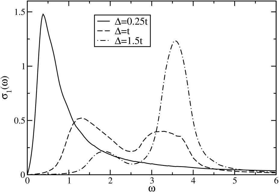
Figure 7: Optical conductivity $\sigma_{1}(\omega)$ for $U=6t$ and $\eta=0.2t$ ($L=32$) for various dimerizations $\Delta$.

3.4 From Small to Large Dimerization

Although the nature of the optical excitations greatly differs in the strong and weak coupling limits, we have found that the evolution of the optical spectrum with $\Delta$ is qualitatively similar for all values of $U>0$. In the strong-coupling limit the spectrum is given by Eq. (9) and thus the evolution of $\sigma_{1}(\omega)$ with $\Delta$ can be described accurately. When the dimerization is weak ($\Delta\ll t$), most of the optical weight is concentrated just above the first singularity at the spectrum onset $\omega=E_{c}=2\Delta$ and the second singularity at $\omega=4t$ carries very little weight. As $\Delta$ increases, the optical weight is progressively transfered from the low-energy singularity to the high-energy one until the spectral weight becomes equally distributed between both singularities as one reaches the large dimerization limit $\Delta\rightarrow 2t$. Simultaneously, the first singularity moves to higher energy as $\Delta$ increases and ultimately merges with the second (fixed) one as $\Delta$ reaches $2t$. Therefore, we observe both a transfer of optical weight from a low-energy structure around $\omega=E_{c}$ to a high-energy structure around $\omega=4t$ and a shift of the low-energy structure toward higher excitation energies as $\Delta$ increases.

Away from the strong-coupling limit Eq. (9) is not an accurate description of the optical spectrum. Nevertheless, our DDMRG calculations show a qualitatively similar evolution of the spectrum as a function of $\Delta$ for all values of $U$ that we have analyzed (i.e., down to $U=t$). For instance, Fig. 7 shows the optical conductivity calculated with DDMRG for $U=6t$ and several values of $\Delta$. We clearly see both the optical weight transfer from the low-energy peak to the high-energy structure and the shift of the low-energy peak toward higher energy as $\Delta$ increases. We note, however, that the low-energy peak is close to the Mott gap $E_{c}$ for small $\Delta$ only. For larger $\Delta$ the position of the first peak moves away from $E_{c}$ (at least when $U$ is not too large) contrary to the strong-coupling result (9). As a result, the dominant features in $\sigma_{1}(\omega)$ can lie well above the Mott gap $E_{c}$ as already shown for the large-dimerization limit in Sec. 3.1. The high-energy structure always lies at an energy close to $4t$ for all $U$ and $\Delta$ but its weight can become so small that it is no longer visible such as in the weak-coupling limit (see Fig. 5).

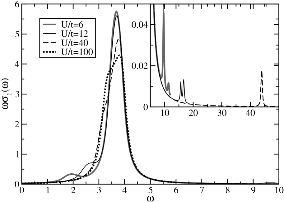
Figure 8: Reduced optical conductivity $\omega\sigma_{1}(\omega)$ calculated with $\eta=0.2t$ ($L=64$) for $\Delta=1.64t$ and various values of $U$. Inset: expanded view of the high-frequency conductivity spectrum.

3.5 From Weak to Strong Coupling

For a given dimerization $\Delta<2t$ the strength $U$ of the local Coulomb interaction significantly modifies the Mott gap $E_{c}$, which is equal to the optical gap for $\Delta<2t$ and $V=0$. However, it has little effect on the main features of the optical spectrum and just modifies the fine structure. For instance, Fig. 8 shows the reduced optical conductivity calculated with DDMRG for $\Delta=1.64t$ and various values of $U$. For $U\leq 4t$ the optical spectrum is well explained by the analysis of the large-dimerization limit (Sec. 3.1). It consists of a strong structure at $\omega\approx 2t_{1}=3.64t$ (the intra-dimer band) and weaker features at $\omega\approx E_{c}$ and $\omega\approx 2t_{1}+U$ (see Fig. 1). When $U$ increases, the gap becomes larger and correspondingly we observe a progressive shift of the low-frequency weak structure toward the strong peak in Fig. 8. Simultaneously, the high-frequency weak feature moves to higher energies in agreement with the relation $\omega\approx 2t_{1}+U$ (see the inset of Fig. 8). However, the strong dominant structure remains largely unaffected by the variation of the coupling $U$.

Nevertheless, the analysis of the optical conductivity for changing $U$ yields an interesting result. As discussed in Sec. 3.3 in the weak-coupling approach the local interaction term is responsible for an (effective) interaction $\propto U$ which splits the (effectively) half-filled band [defined by the lower part of the single-particle dispersion (2)] in two (effective) Hubbard bands separated by a gap $E_{c}$. Excitations from the lower to the upper effective Hubbard bands significantly contribute to the optical spectrum on the energy scale $\omega=E_{c}$. In the strong-coupling approach the local interaction term splits the full band defined by the dispersion (2) in two (full) Hubbard bands separated by a gap $\sim U$. In that case, excitations from the lower to the upper full Hubbard bands contribute to the optical spectrum around $\omega=U$. Our calculations show that both features can be seen (for instance, in Figs. 1 and 8) for a given value of $U$. Therefore, we conclude that, at least for some parameters ($\Delta,U$) of the model (2), the low-frequency part of the optical spectrum is explained by weak-coupling (i.e., field-theoretical) approaches while the high-frequency part is explained by a strong-coupling analysis.

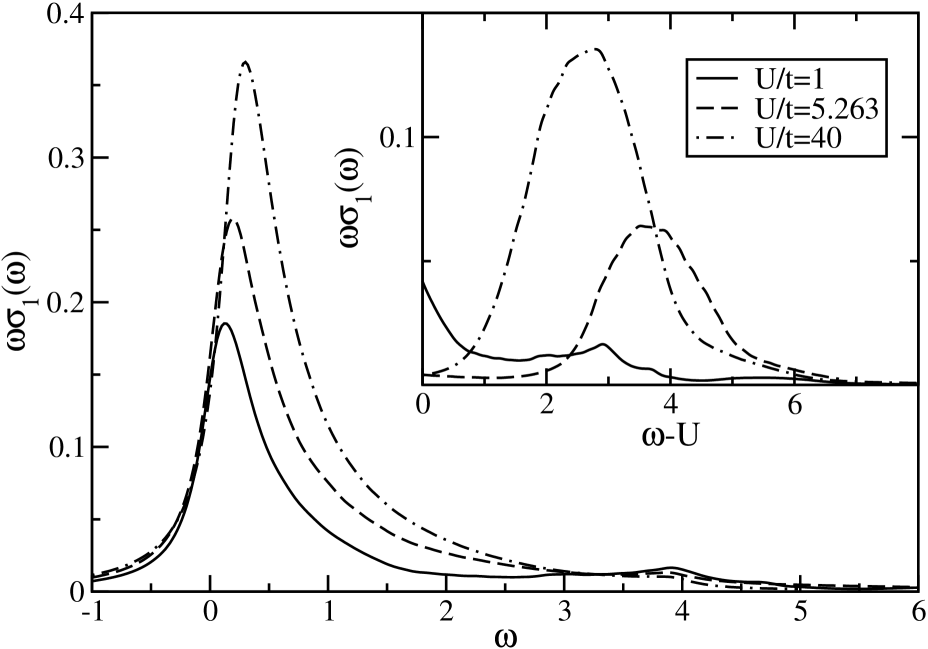
Figure 9: Reduced optical conductivity $\omega\sigma_{1}(\omega)$ calculated with $\eta=0.2t$ ($L=64$) for $\Delta=0.105t$ and various values of $U$. Inset: expanded view of the high-frequency conductivity spectrum as a function of $\omega-U$.

As a second example of the optical spectrum evolution with $U$, we show the reduced optical conductivity calculated with DDMRG for a small dimerization $\Delta=0.105t$ and various interaction strengths $U$ in Fig. 9. For $U=t$ the system is in the weak-coupling limit (discussed in Sec. 3.3) and most of the spectral weight is concentrated in a peak close to $\omega=E_{c}$. A second weaker feature is visible at about $\omega=4t$ (see the inset of Fig. 9) and corresponds to transitions from the bottom to the top of the single-particle band (2). For larger $U$ the optical weight remains concentrated in the low-energy peak at $\omega\approx E_{c}$. This peak moves to slightly higher energies and appears to broaden because the energy scale set by the gap $E_{c}$ increases with $U$ until it reaches $2\Delta$ for $U\rightarrow\infty$ as discussed in Sec. 3.2 but its shape is not significantly changed by the variation of $U$. The feature at $\omega\approx 4t$ disappears for $U>4t$ but another weak feature becomes visible around $\omega\approx U$ for strong enough coupling $U$ (see the inset of Fig. 9). Again this corresponds to optical excitations from the lower to the upper (full) Hubbard bands.

We note that for $U=5.263t$ this contribution to the optical spectrum is already clearly visible around $\omega-U=4t$ in the inset of Fig. 9. This result contradicts the apparent asymptotic power-law decrease (10) discussed previously for the same parameters (see Fig. 5). This discrepancy is due to the different broadening methods and data representation used for Figs. 5 and 9. It confirms that the asymptotic power law found in some of our spectra for weak couplings are probably an artifact of the broadening used in the DDMRG calculation. This also illustrates how difficult it is to observe the field-theoretical predictions (10) for the asymptotic behavior of $\sigma_{1}(\omega)$ in the lattice model (2) because optical transitions neglected in the field theory approach significantly contributes to the high-frequency spectrum.

In summary, our calculations for the model (2) with $V=0$ show that the distribution of the optical weight is essentially determined by the dimerization amplitude $\Delta$. For a fixed $\Delta$ only the fine structure of the optical spectrum and the energy scale set by the gap $E_{c}$ depend significantly on $U$.

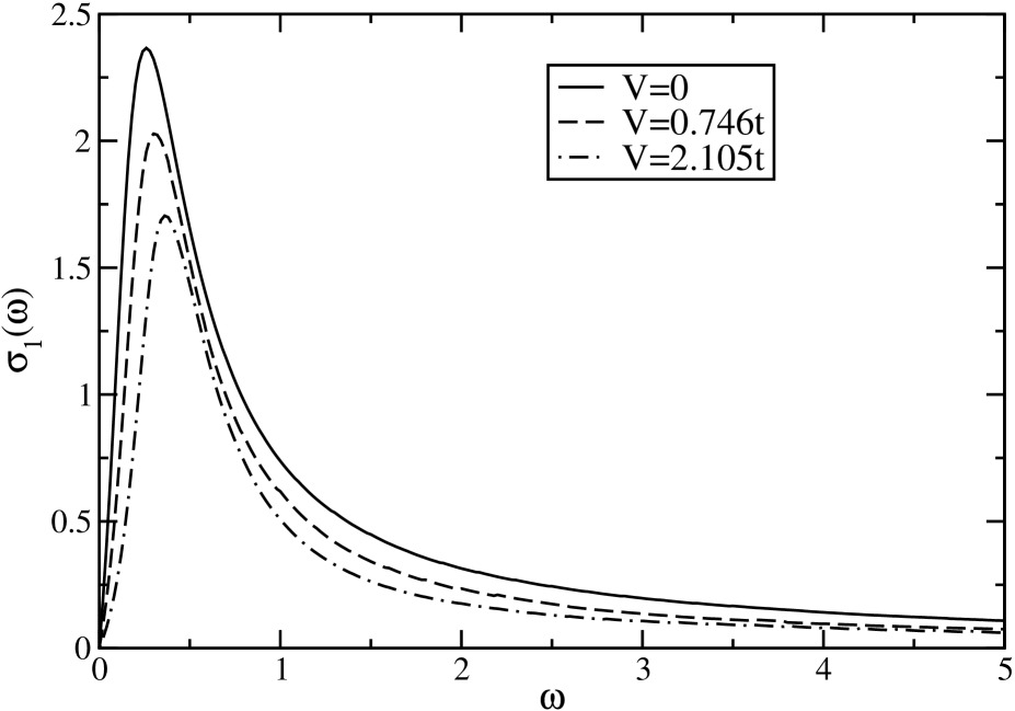
Figure 10: Optical conductivity $\sigma_{1}(\omega)$ for $\Delta=0.105t$, $U=5.263t$, $\eta=0.2t$ ($L=64$), and various nearest-neighbor interactions $V$.

3.6 Nearest-Neighbor Interaction

Neglecting the long-range part of the Coulomb interaction is difficult to justify in an insulator. In this section we consider the effects of a nearest-neighbor repulsion $V>0$ in the Hamiltonian (2). (This term mimics the long-range part of the Coulomb interaction.) For large enough $V$ the nature of the ground state of (2) changes from a Mott insulator to a CDW insulator shi01 . Here we discuss only the optical conductivity in the Mott insulating phase.

A previous DMRG investigation nis00 of the model (2) has shown that the charge gap $E_{c}$ increases with $V$ in the Mott insulating phase. Our calculations confirm this result. For $V=0$ (and $\Delta<2t$) the optical gap $\omega_{1}$ is equal to the Mott gap $E_{c}$ in the thermodynamic limit (see Fig. 6 for an example). This gap marks the onset of an excitation continuum of unbound pairs of elementary charged excitations (for instance, holon-antiholon pairs in the weak-coupling picture con01 ) which are responsible for the lowest absorption band in the optical conductivity. We have found that the optical gap remains equal to the Mott gap for non-zero but small nearest-neighbor repulsion $V$. Thus, the low-energy spectrum still corresponds to unbound pairs of charged excitations.

Figure 11: Mott gap $E_{c}$ (circle), optical gap $\omega_{1}$ (square), and position $\omega_{\rm max}$ of the spectrum maximum (cross) as a function of the inverse system size for (a) $\Delta=0.105t,U=5.263t,$ and $V=2.105t$, and (b) $\Delta=0.353t,U=8.235t,V=3.294t$. Lines are quadratic fits.

Figure 10 illustrates two main effects of the nearest-neighbor repulsion on the optical spectrum for small $V$. First, the low-frequency peak above $E_{c}$ is shifted to higher frequency as $V$ increases because $E_{c}$ also increases. Secondly, the total spectral weight decreases with increasing $V$ as described in Ref. mil95 .

For stronger coupling $V$, however, we have found that the optical gap extrapolates to a smaller value than the Mott gap in the limit of an infinite chain. This can be seen in Fig. 11. In the first example (for $\Delta=0.105t,U=5.263t$, and $V=2.105t$) the difference $E_{b}=\omega_{1}-E_{c}$ is small (about $0.04t$) but in the second example (for $\Delta=0.353t,U=8.235t$, and $V=3.294t$) it is large ($E_{b}\approx 0.9t$). Moreover, the maximum of the optical spectrum is located at a frequency $\omega_{\rm max}$ which approaches the same value as $\omega_{1}$ in the thermodynamic limit. This is the signature of a excitonic peak ($\delta$-peak) at $\omega=\omega_{1}$ in the optical spectrum of the Mott insulator. (See Refs. jec02 ; ess01 ; jec03 for a description of the analysis that allows us to identify an excitonic peak in a DDMRG spectrum.) The presence of an excitonic peak signals a fundamental change in the nature of the lowest optical excitation. It is now a neutral bound pair (for instance, a bound holon-antiholon pair in field theory) called a Mott-Hubbard exciton ess01 . The properties of Mott-Hubbard excitons have been investigated using DDMRG and analytical methods in a previous work ess01 . The exciton energy $\omega_{1}$ is smaller than the excitation energy of the lowest unbound pair of charged excitations in the continuum (which is $E_{c}$). The difference $E_{b}=\omega_{1}-E_{c}$ is the binding energy of the exciton. Therefore, the first example in Fig. 11 corresponds to a weakly bound (large) Mott-Hubbard exciton while the second example corresponds to a tightly bound (small) one.

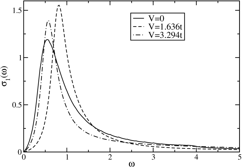
Figure 12: Optical conductivity $\sigma_{1}(\omega)$ for $\Delta=0.353t$, $U=8.235t$, $\eta=0.2t$ ($L=64$), and various nearest-neighbor interactions $V$.

The exciton generates a $\delta$-peak at $\omega=\omega_{1}<E_{c}$ in the optical conductivity spectrum. As $V$ increases the exciton becomes more tightly bound (smaller) and the optical weight is progressively transfered from the continuum above $E_{c}$ to the excitonic peak. In Fig. 12 one sees that the optical weight first moves to higher frequency as one increases the coupling $V$ form 0 to $1.636t$ because the Mott gap $E_{c}$ (i.e., the continuum onset) increases. If the coupling $V$ is increased further to $3.294t$, one finds that the spectral weight shifts to lower frequency because it is transfered to the excitonic peak at $\omega_{1}\approx 0.5t$ lying below the continuum onset at $E_{c}=1.4t$ (which still increases with $V$). (Note that the gap between the exciton peak and the continuum is not visible in Fig. 12 for $V=3.294t$ because of the broadening of the spectrum.) The (weak) structure visible at $\omega\approx 4t$ in the spectra calculated for $V=0$ rapidly looses weight as $V$ increases. In summary, we have found that the nearest-neighbor repulsion $V$ has a significant impact on the shape of the optical spectrum contrary to the on-site repulsion, but only when it is large enough to generate an exciton.

4 Discussion

In this section we discuss the implications of our results for the theory of the Bechgaard salts. First, we examine which values of the model parameters could be appropriate for (TM)₂X salts. Realistic estimates for the hopping integrals $t_{1}$ and $t_{2}$ were proposed more than ten years ago on the basis of experimental results ped94 and quantum-chemistry calculations duc86 . Using these estimates Mila mil95 determined the model parameters $U$ and $V$ from the reduction of the infrared oscillator strength observed experimentally in the Bechgaard salts. He found that relatively large nearest-neighbor repulsions $V$ were necessary to explain the reduction of the electron kinetic energy due to correlation effects. According to Mila’s analysis appropriate model parameters are $t_{2}/t_{1}=0.9$, $U=5t_{1}$, and $V=2t_{1}$, which correspond to $\Delta=0.105t$, $U=5.263t$, and $V=2.105t$, for (TMTSF)₂ClO₄ and $t_{2}/t_{1}=0.7$, $U=7t_{1}$, and $V=2.8t_{1}$, which correspond to $\Delta=0.353t$, $U=8.235t$, and $V=3.294t$, for (TMTTF)₂PF₆. The optical spectrum obtained with DDMRG for these parameters are shown in Figs. 10 and 12, respectively. As explained in Sec. 3.6 we have found that the lowest optical excitation is an exciton with an energy $\omega_{1}$ smaller than the Mott gap $E_{c}$ for these parameters (see Fig. 11).

More recently, Nishimoto et al. nis00 fitted the Mott gap of the model (2) to the experimental optical gap to determine the model parameters. Using the same ratios $t_{2}/t_{1}$ and $U/t_{1}$ as Mila they found that the nearest-neighbor repulsions $V$ necessary to reproduce the optical gap data were significantly smaller than the values given by the reduction of the oscillator strength. According to their analysis $V=0.764t$ for (TMTSF)₂ClO₄ and $V=1.636t$ for (TMTTF)₂PF₆. The optical spectrum obtained with DDMRG for these parameters are also shown in Figs. 10 and 12, respectively. In that case we have found that there is no exciton and an absorption continuum due to unbound pairs of charged excitations starts at $\omega=\omega_{1}=E_{c}$.

The discrepancy between these studies can be understood. In the (TMTSF)₂ClO₄ case the kinetic energy is a rather flat function of $V$ for the relevant parameters $t_{1},t_{2},U$ mil95 while the Mott gap increases rapidly with $V$ nis00 . Thus, the uncertainty on Mila’s value for $V$ is quite large and the value $V=0.764t$ reported by Nishimoto et al. is also compatible with the experimental reduction of the oscillator strength. Therefore, we conclude that for the salt (TMTSF)₂ClO₄ the nearest-neighbor interaction should be close to (though somewhat larger than) the value given by Nishimoto et al. and excitons do not play any role in the optical excitation spectrum. The appropriate model parameters for (TMTSF)₂ClO₄ are summarized in Table 1.

In the (TMTTF)₂PF₆ case, however, the kinetic energy is a rather steep function of $V$ for the relevant parameters $t_{1},t_{2},U$ mil95 and the value $V=1.636t$ found by Nishimoto et al. is only compatible with the oscillator strength reduction for unrealistically large $U$. As Nishimoto et al. assumed that the experimental optical gap corresponded to the theoretical Mott gap $E_{c}$, they effectively neglected excitonic contributions to the optical spectrum. In particular, their analysis does not take into account that the theoretical optical gap $\omega_{1}$ is significantly smaller than the Mott gap $E_{c}$ for large $V$ when excitons occur, as seen in Fig. 11(b). As a result their analysis underestimates the value of $V$. Therefore, we conclude that for (TMTTF)₂PF₆ the nearest-neighbor interaction should be close to (though somewhat smaller than) the value $V=3.294t$ found by Mila and excitons dominate the optical excitation spectrum [at least in the framework of the model (2)]. The appropriate model parameters for (TMTTF)₂PF₆ are summarized in Table 1.

We now examine how the main features of the optical spectrum in (TM)₂X salts can be explained by the dimerized extended Hubbard model with the parameters determined above. Parallel to the stacks of organic molecules the optical conductivity of (TMTSF)₂X salts has two distinct components: a narrow peak at zero frequency (Drude peak) with a very small fraction (about 1 %) of the spectral weight and an absorption band with most of the spectral weight at finite energy dre96 ; ves98 ; sch98 ; ves00 . This second feature lies in the mid infrared range above the crossover energy above which excitations are effectively confined to a single stack and thus can be described by one-dimensional models. (Obviously, the zero-energy feature always lies below such a crossover energy and can only be described in the framework of a three-dimensional model.) The finite-energy feature is usually interpreted in terms of a Mott insulator. When rescaled by the intensity and frequency of the spectrum maximum, the optical conductivity of various (TMTSF)₂X salts exhibit a remarkably similar behavior sch98 . In particular, a power law in the frequency dependence

$$\frac{\sigma_{1}(\omega)}{\sigma_{1}(\omega_{\rm max})}=C\left(\frac{\omega}{\omega_{\rm max}}\right)^{-1.3}$$ (11)

is observed over a decade in frequency $2\omega_{\rm peak}<\omega<20\omega_{\rm peak}$.

As discussed in Sec. 3.3 our numerical approach is not sufficiently accurate to confirm the existence of such an asymptotic power-law behavior in the optical spectrum of the model (2). Nevertheless, our analysis clearly indicates that if there is a power-law behavior of $\sigma_{1}(\omega)$ for some frequency range in the model (2), the optical weight associated with that feature must be extremely small compared to the optical weight of the peak feature. In the experimental spectrum, however, there is substantial optical weight in the region where the power-law behavior is visible. Therefore, we conclude that the universal feature (11) of the optical spectrum in (TMTSF)₂X salts cannot be explained within the model (2).

The well-defined mid infrared structure observed in the optical spectrum of the Bechgaard salt (TMTSF)₂PF₆ is difficult to understand in view of the fact that its DC conductivity remains metallic down to very low temperature. It seems that optical excitations are visible only for energies much larger than the energy scale above which the system can be seen as metallic (i.e., the Mott gap for charge excitations). Therefore, Favand and Mila fav96 have proposed that the optical gap $\omega_{1}$ observed in the absorption spectrum is much larger than the Mott gap $E_{c}$ because of optical selection rules. Using exact diagonalizations of small systems they have argued that such an effect occurs in the quarter-filled dimerized Hubbard model (2) without the nearest-neighbor repulsion $V$. Our analysis of this model shows that the Mott gap is smaller than the optical gap only in the dimer case $\Delta=2t$ (see the discussion in Sec. 3.1). For all other parameters $(t_{1},t_{2},U)$, however, we have found that $\omega_{1}=E_{c}$ ($\omega_{1}<E_{c}$ is also possible for $V>0$ as shown in Sec. 3.6). It can happen that the optical weight at the Mott gap is very small while a very strong structure is visible in the spectrum at a higher energy. For instance, this occurs in the large-dimerization limit as seen in Fig. 1. In a real material with such an absorption spectrum the weak low-energy band could easily be overlooked, leading to an apparent “optical gap” larger than the real gap for charge excitations $E_{c}$. For realistic parameters, however, we always find that the optical weight is very large close to the Mott gap. In particular, for the parameters $t_{2}=0.9t_{1}$ and $U=5t_{1}$ ($\Delta=0.105t$ and $U=5.263t$) used by Favand and Mila for (TMTSF)₂PF₆ (see Table 1) we have found that the Mott gap, the optical gap, and the maximum of the spectrum converge to very close values in the thermodynamic limit (see Fig. 6). We conclude that the model (2) cannot explain the apparent discrepancy between energy scales in the optical spectrum and the conductivity measurements for the Bechgaard salt (TMTSF)₂PF₆.

Parallel to the stacks of organic molecules the optical properties of (TMTTF)₂X salts are clearly those of semiconductors ves98 ; ves00 . The optical spectrum displays several strong absorption features which are attributed to the coupling of electronic excitations with lattice vibrations. These transitions have a higher energy than the crossover energy above which excitations are effectively confined to a single stack and thus can be described by a one-dimensional model. A remarkable property of the (TMTTF)₂X salts is that the optical gap is smaller than the Mott gap determined by photoemission experiments. For (TMTTF)₂PF₆ one observes that the strongest structure in the optical spectrum is a relatively sharp peak at an energy (about 100 meV) significantly smaller than the Mott gap (about 200 meV). Obviously, this can be interpreted as the signature of an excitonic transition below the gap for charged excitations. Thus, experimental observations are compatible with the theoretical prediction of excitons in (TMTTF)₂PF₆ based on the model (2) and Mila’s estimation mil95 for the appropriate parameters (especially, the strength of the nearest-neighbor interaction $V$). Quantitatively, we find $E_{c}\approx 160$ meV and an exciton energy of $\omega_{1}\approx$ 60 meV using the parameters in Table 1. These energies are in very satisfactory agreement with the experimental values. Therefore, we conclude that excitons are present in the optical spectrum of (TMTTF)₂PF₆ [and probably other (TMTTF)₂X salts] and explain the observation of absorption features below the gap measured with photoemission spectroscopy. It would be interesting to have a direct experimental evidence for the presence of excitons in those salts. For instance, one could investigate the electro-absorption spectrum to demonstrate the presence of excitons as it was done for another quasi-one-dimensional material, polydiacetylene weiser .

In conclusion, we have investigated the optical conductivity of the one-dimensional dimerized extended Hubbard model at quarter filling using the dynamical density-matrix renormalization group. We have found that the dimerization amplitude and the nearest-neighbor repulsion (if strong enough to form excitons) determine the main features of the optical spectrum. Besides its influence on the energy scale set by the Mott gap, the on-site repulsion plays a minor role only. Our study shows that this model cannot explain the optical spectrum in the Bechgaard salts (TMTSF)₂X. It also shows that excitons probably contribute to the optical spectrum in the (TMTTF)₂X salts.

Acknowledgments

We are grateful to S. Nishimoto, F. Gebhard, and F. Mila for helpful discussions. H.B. acknowledges support by the Optodynamics Center of the Philipps-Universität Marburg.

References

- (1) J.-P. Farges (Ed.), Organic Conductors (Marcel Dekker, New York, 1994)
- (2) T. Ishiguro, K. Yamaji, and G. Saito, Organic Superconductors (Springer, Berlin, 1998)
- (3) C. Bourbonnais and D. Jérome, in Advances in Synthetic Metals, Twenty Years of Progress in Science and Technology, edited by P. Bernier, S. Lefrant, and G. Bidan (Elsevier, New York, 1999), pp. 206-301
- (4) K. Penc and F. Mila, Phys. Rev. B 50, 11429 (1994)
- (5) F. Mila, Phys. Rev. B 52, 4788 (1995)
- (6) J. Favand and F. Mila, Phys. Rev. B 54, 10425 (1996)
- (7) S. Nishimoto, M. Takahashi, and Y. Ohta, J. Phys. Soc. Jpn. 69, 1594-1597 (2000)
- (8) Y. Shibata, S. Nishimoto, and Y. Ohta, Phys. Rev. B 64, 235107 (2001)
- (9) M. Tsuchiizu, H. Yoshioka, and Y. Suzumura, J. Phys. Soc. Jpn. 70, 1460-1463 (2001)
- (10) D. Pedron, R. Bozio, M. Meneghetti, and C. Pecile, Phys. Rev. B 49, 10893 (1994)
- (11) M. Dressel, A. Schwartz, G. Grüner, and L. Degiorgi, Phys. Rev. Lett 77, 398 (1996)
- (12) V. Vescoli, L. Degiorgi, W. Henderson, G. Grüner, K.P. Starkey, and L.K. Montgomery, Science 281, 181 (1998)
- (13) A. Schwartz, M. Dressel, G. Grüner, V. Vescoli, L. Degiorgi, and T. Giamarchi, Phys. Rev. B 58, 1261 (1998)
- (14) V. Vescoli, F. Zwick, W. Henderson, L. Degiorgi, M. Grioni, G. Grüner, and L.K. Montgomery, Eur. Phys. J. B 13, 503-511 (2000)
- (15) E. Jeckelmann, F. Gebhard, and F.H.L. Essler, Phys. Rev. Lett. 85, 3910-3913 (2000)
- (16) D. Controzzi, F.H.L. Essler, and A.M. Tsvelik, Phys. Rev. Lett. 86, 680 (2001)
- (17) T. Giamarchi, Phys. Rev. B 46, 342 (1992); Physica B 230-232, 975 (1997)
- (18) E. Jeckelmann, Phys. Rev. B 66, 045114 (2002)
- (19) L. Ducasse et al., J. Phys. C: Solid State Phys. 19, 3805 (1986)
- (20) S.R. White, Phys. Rev. Lett. 69, 2863 (1992); Phys. Rev. B 48, 10345 (1993)
- (21) I. Peschel, X. Wang, M. Kaulke, and K. Hallberg (Eds.), Density-Matrix Renormalization (Springer, Berlin, 1999)
- (22) J.E. Hirsch and D.J. Scalapino, Phys. Rev. B 29, 5554 (1984)
- (23) F. Mila and X. Zotos, Europhys. Lett. 24, 133-138 (1993)
- (24) F.H.L. Essler, F. Gebhard, and E. Jeckelmann, Phys. Rev. B 64, 125119 (2001)
- (25) E. Jeckelmann, Phys. Rev. B 67, 075106 (2003)
- (26) Young-June Kim, J.P. Hill, H. Benthien, F.H.L. Essler, E. Jeckelmann, H.S. Choi, T.W. Noh, N. Motoyama, K.M. Kojima, S. Uchida, D. Casa, and T. Gog, Phys. Rev. Lett. 92, 137402 (2004)
- (27) F. Gebhard, E. Jeckelmann, S. Mahlert, S. Nishimoto, and R.M. Noack, Eur. Phys. J. B 36, 491-509 (2003)
- (28) C. Raas and G.S. Uhrig, cond-mat/0412224 (2004)
- (29) W.H. Press, S.A. Teukolsky, W.T. Vetterling, and B.P. Flannery, Numerical Recipes in C++ (Cambridge University Press, Cambridge, 2002)
- (30) F. Gebhard, K. Bott, M. Scheidler, P. Thomas, and S.W. Koch, Philos. Mag. B 75, 47 (1997)
- (31) F. Gebhard, K. Bott, M. Scheidler, P. Thomas, and S.W. Koch, Philos. Mag. B 75, 1 (1997)
- (32) G. Weiser, Phys. Rev. B 45, 14076 (1992)