What entropy at the edge of chaos?

Abstract

Numerical experiments support the interesting conjecture that statistical methods be applicable not only to fully-chaotic systems, but also at the edge of chaos by using Tsallis’ generalizations of the standard exponential and entropy. In particular, the entropy increases linearly and the sensitivity to initial conditions grows as a generalized exponential. We show that this conjecture has actually a broader validity by using a large class of deformed entropies and exponentials and the logistic map as test cases.

Chaotic systems at the edge of chaos constitute natural experimental laboratories for extensions of Boltzmann-Gibbs statistical mechanics. The concept of generalized exponential could unify power-law and exponential sensitivity to initial conditions leading to the definition of generalized Liapounov exponents [1]: the sensitivity $\xi\equiv\lim_{t\to\infty}\lim_{\Delta x(0)\to 0}\Delta x(t)/\Delta x(0)\sim\widetilde{\exp}(\lambda t)$, where the generalized exponential $\widetilde{\exp}(x)=\exp_{q}(x)=[1+(1-q)x]^{1/(1-q)}$; the exponential behavior for the fully-chaotic regime is recovered for $q\to 1$: $\lim_{q\to 1}\exp_{q}(\lambda_{q}t)=\exp(\lambda t)$. Analogously, a generalization of the Kolmogorov entropy should describe the relevant rate of loss of information. A general discussion of the relation between the Kolmogorov-Sinai entropy rate and the statistical entropy of fully-chaotic systems can be found in Ref. Latora:1999prl: asymptotically and for ideal coarse graining, the entropy grows linearly with time. The generalized entropy proposed by Tsallis [3] $S_{q}=(1-\sum_{i=1}^{N}p_{i}^{q})/(q-1)$, with $p_{i}$ the fraction of the ensemble found in the $i$-th cell, reproduces this picture at the edge of chaos; it grows linearly for a specific value of the entropic parameter $q=q_{\mathrm{sens}}=0.2445$ in the logistic map: $\lim_{t\to\infty}\lim_{L\to 0}S_{q}(t)/t=K_{q}$. The same exponent describes the asymptotic power-law sensitivity to initial conditions [4]. This conjecture includes an extension of the Pesin identity $K_{q}=\lambda_{q}$. Numerical evidences with the entropic form $S_{q}$ exist for the logistic [1] and generalized logistic-like maps [5].

Renormalization group methods [6] yield the asymptotic exponent of the sensitivity to initial conditions in the logistic and generalized logistic maps for specific initial conditions on the attractor; the Pesin identity for Tsallis’ entropy has been also studied [7].

Sensitivity and entropy production have been studied in one-dimensional dissipative maps using ensemble-averaged initial conditions [8] and for two simpletic standard maps [9]: the statistical picture has been confirmed with a different $q=q_{\mathrm{sens}}^{\mathrm{ave}}=0.35$ [8]. The ensemble-averaged initial conditions is relevant for the relation between ergodicity and chaos and for practical experiments.

The present study demonstrates the broader applicability of the above-described picture by using the consistent statistical mechanics arising from the two-parameter family [10, 11, 12, 13] of logarithms

$$\widetilde{\ln}(\xi)\equiv\frac{\xi^{\alpha}-\xi^{-\beta}}{\alpha+\beta}\quad.$$ (1)

Physical requirements [14] on the resulting entropy select [15] $0\leq\alpha\leq 1$ and $0\leq\beta<1$. All the entropies of this class: (i) are concave [12], (ii) are Lesche stable [16], and (iii) yield normalizable distributions [15]; in addition, we shall show that they (iv) yield a finite non-zero asymptotic rate of entropy production for the logistic map with the appropriate choice of $\alpha$.

We have considered the whole class, but we shall here report results for three interesting one-parameter cases:

(1) the original Tsallis proposal [3] ($\alpha=1-q$, $\beta=0$):

$$\widetilde{\ln}(\xi)=\ln_{q}(\xi)\equiv\frac{\xi^{1-q}-1}{1-q}\quad;$$ (2)

(2) Abe’s logarithm

$$\widetilde{\ln}(\xi)=\ln_{A}(\xi)\equiv\frac{\xi^{1/q_{A}-1}-\xi^{q_{A}-1}}{1/q_{A}-q_{A}}\quad,$$ (3)

where $q_{A}=1/(1+\alpha)$ and $\beta=\alpha/(1+\alpha)$, which has the same quantum-group symmetry of and is related to the entropy introduced in Ref. Abe:1997qg;

(3) and Kaniadakis’ logarithm, $\alpha=\beta=\kappa$, which shares the same symmetry group of the relativistic momentum transformation [18]

$$\widetilde{\ln}(\xi)=\ln_{\kappa}(\xi)\equiv\frac{\xi^{\kappa}-\xi^{-\kappa}}{2\kappa}\quad.$$ (4)

The sensitivity to initial conditions and the entropy production has been studied in the logistic map $x_{i+1}=1-\mu x^{2}_{i}$ at the infinite-bifurcation point $\mu_{\infty}=1.401155189$. The generalized logarithm $\widetilde{\ln}(\xi)$ of the sensitivity, $\xi(t)=(2\mu)^{t}\prod_{i=0}^{t-1}|x_{i}|$ for $1\leq t\leq 80$, has been uniformly averaged by randomly choosing $4\times 10^{7}$ initial conditions $-1<x_{0}<1$. Analogously to the chaotic regime, the deformed logarithm of $\xi$ should yield a straight line $\widetilde{\ln}(\xi(t))=\widetilde{\ln}(\widetilde{\exp}(\lambda t))=\lambda t$.

Following Ref. Ananos:2004a, where the exponent obtained with this averaging procedure, indicated by $\langle\cdots\rangle$, was denoted $q_{\mathrm{sens}}^{\mathrm{av}}$ for Tsallis’ entropy, each of the generalized logarithms, $\langle\widetilde{\ln}(\xi(t))\rangle$, has been fitted to a quadratic function for $1\leq t\leq 80$ and $\alpha$ has been chosen such that the coefficient of the quadratic term be zero: we call this value $\alpha^{\mathrm{av}}_{\mathrm{sens}}$.

Statistical errors, estimated by repeating the whole procedure with sub-samples of the $4\times 10^{7}$ initial conditions, and systematic uncertainties, estimated by including different numbers of points in the fit, have been quadratically combined.

We find that the asymptotic exponent $\alpha^{\mathrm{av}}_{\mathrm{sens}}=0.650\pm 0.005$ is consistent with the value of Ref. Ananos:2004a: $q^{\mathrm{av}}_{\mathrm{sens}}=1-\alpha^{\mathrm{av}}_{\mathrm{sens}}\approx 0.36$. The error on $\alpha^{\mathrm{av}}_{\mathrm{sens}}$ is dominated by the systematic one (choice of the number of points) due to the inclusion of small values of $\xi$ which produces 1% discrepancies from the common asymptotic behavior.

Figure 1 shows the straight-line behavior of $\widetilde{\ln}(\xi)$ for all formulations when $\alpha=\alpha^{\mathrm{av}}_{\mathrm{sens}}$ (right frame); the corresponding slopes $\lambda$ (generalized Lyapunov exponents) are $0.271\pm 0.004$ (Tsallis), $0.185\pm 0.004$ (Abe) and $0.148\pm 0.004$ (Kaniadakis). While $\alpha$ is a universal characteristic of the map, the slope $\lambda$ strongly depends on the choice of the logarithm.

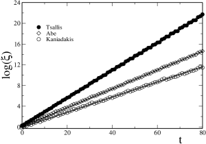
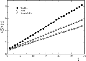
Figure 1: Generalized logarithm of the sensitivity to initial conditions (left) and generalized entropy (right) as function of time. From top to bottom, Tsallis’, Abe’s and Kaniadakis’ logarithms (entropies) for $\alpha=\alpha^{\mathrm{av}}_{\mathrm{sens}}$. In the left frame the slopes $\lambda$ (generalized Lyapunov exponents) are $0.271\pm 0.004$, $0.185\pm 0.004$ and $0.148\pm 0.004$; in the right frame the slopes $K$ (generalized Kolmogorov entropies) are $0.267\pm 0.004$, $0.186\pm 0.004$ and $0.152\pm 0.004$.

The entropy has been calculated by dividing the interval $(-1,1)$ in $W=10^{5}$ equal-size boxes, putting at the initial time $N=10^{6}$ copies of the system with a uniform random distribution within one box, and then letting the systems evolve according to the map. At each time $p_{i}(t)\equiv n_{i}(t)/N$, where $n_{i}(t)$ is the number of systems found in the box $i$ at time $t$, the entropy of the ensemble is

$$S(t)\equiv\left\langle\sum_{i=1}^{N}p_{i}(t)\widetilde{\ln}(\frac{1}{p_{i}(t)})\right\rangle=\left\langle\sum_{i=1}^{N}\frac{p_{i}^{1-\alpha}(t)-p_{i}^{1+\beta}(t)}{\alpha+\beta}\right\rangle$$ (5)

where $\langle\cdots\rangle$ is an average over $2\times 10^{4}$ experiments, each one starting from one box randomly chosen among the $N$ boxes. The application of the MaxEnt principle to the entropy (5) yields as distribution the deformed exponential that is the inverse function of the corresponding logarithm of Eq. (1): $\widetilde{\exp}(x)=\widetilde{\ln}^{-1}(x)$ [15].

Analogously to the strong chaotic case, where an exponential sensibility ($\alpha=\beta=0$) is associated to a linear rising Shannon entropy, which is defined in terms of the usual logarithm ($\alpha=\beta=0$), we use the same values $\alpha$ and $\beta$ of the sensitivity for the entropy of Eq. (5). Fig. 1 shows (right frame) that this choice leads to entropies that grow linearly: the corresponding slopes $K$ (generalized Kolmogorov entropies) are $0.267\pm 0.004$ (Tsallis), $0.186\pm 0.004$ (Abe) and $0.152\pm 0.004$ (Kaniadakis). This linear behavior disappears when $\alpha\neq\alpha^{\mathrm{av}}_{\mathrm{sens}}$ as shown in Fig. 2 for Tsallis’, Abe’s and Kaniadakis’ entropies.

In addition, the whole class of entropies and logarithms verifies the Pesin identity $K=\lambda$ confirming what was already known for Tsallis’ formulation [1, 8]. The values of $\lambda$ and $K$ for the specific Tsallis’, Abe’s and Kaniadakis formulations are given in the caption to Fig. 1 as important explicit examples of this identity.

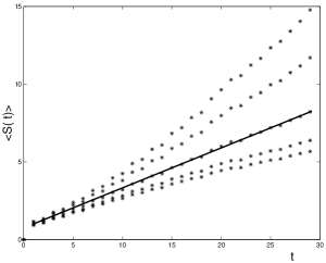
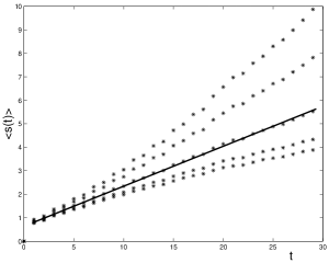
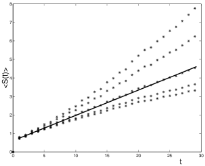
Figure 2: Tsallis’ (top left), Abe’s (top right) and Kaniadakis’ (bottom) entropies as function of time for $\alpha=1-q=0.80$, 0.74, 0.64, 0.56, 0.52 (from top to bottom). Straight lines are guides for the eyes when $\alpha=0.64\approx\alpha^{\mathrm{av}}_{\mathrm{sens}}$.

An intuitive explanation of the dependence of the value of $K$ on $\beta$ and details on the calculations can be found in Ref. Tonelli:2004ha.

In summary, numerical evidence corroborates and extends Tsallis’ conjecture that, analogously to strongly chaotic systems, also weak chaotic systems can be described by an appropriate statistical formalism. In addition to sharing the same asymptotic power-law behavior to correctly describe chaotic systems, extended formalisms should verify precise theoretical requirements.

These requirements define a large class of entropies; within this class we use the two-parameter formula (5), which includes Tsallis’s seminal proposal. Its simple power-law form describes both small and large probability behaviors. Specifically, the logistic map shows:

(a) a power-low sensitivity to initial conditions with a specific exponent $\xi\sim t^{1/\alpha}$, where $\alpha=0.650\pm 0.005$; this sensitivity can be described by deformed exponentials with the same asymptotic behavior $\xi(t)=\widetilde{\exp}(\lambda t)$ (see Fig. 1, left frame);

(b) a constant asymptotic entropy production rate (see Fig. 1, right frame) for trace-form entropies that go as $p^{1-\alpha}$ in the limit of small probabilities $p$, where $\alpha$ is the same exponent of the sensitivity;

(c) the asymptotic exponent $\alpha$ is related to parameters of known entropies: $\alpha=1-q$, where $q$ is the entropic index of Tsallis’ thermodynamics [3]; $\alpha=1/q_{A}-1$, where $q_{A}$ appears in the generalization (3) of Abe’s entropy [17]; $\alpha=\kappa$, where $\kappa$ is the parameter in Kaniadakis’ statistics [18];

(d) Pesin identity holds $S_{\beta}/t\to K_{\beta}=\lambda_{\beta}$ for each choice of entropy and corresponding exponential in the class, even if the value of $K_{\beta}=\lambda_{\beta}$ depends on the specific entropy and it is not characteristic of the map as it is $\alpha$ [19];

(e) this picture is not valid for every entropy: an important counterexample is the Renyi entropy , $S_{q}^{(R)}(t)=\left\langle(1-q)^{-1}\log\left[\sum_{i=1}^{N}p_{i}^{q}(t)\right]\right\rangle$, which has a non-linear behavior for any choice of the parameter $q=1-\alpha$ (see Fig. 3).

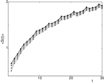
Figure 3: Renyi’s entropy for $0.1\leq\alpha=1-q\leq 0.95$ (from top to bottom).

We gratefully thank S. Abe, F. Baldovin, G. Kaniadakis, G. Mezzorani, P. Quarati, A. Robledo, A. M. Scarfone, U. Tirnakli, and C. Tsallis for suggestions and comments.

References

- [1] C. Tsallis, A. R. Plastino, and W.-M. Zheng, Chaos Solitons Fractals 8, 885 (1997).
- [2] V. Latora and M. Baranger, Phys. Rev. Lett. 82, 520 (1999).
- [3] C. Tsallis, J. Statist. Phys. 52, 479 (1988).
- [4] V. Latora, M. Baranger, A. Rapisarda and C. Tsallis, Phys. Lett. A 273, 97 (2000).
- [5] U. M.S. Costa, M. L. Lyra, A. R. Plastino and C. Tsallis, Phys. Rev. E 56, 245 (1997).
- [6] F. Baldovin and A. Robledo, Phys. Rev. E 66, 045104 (2002); Europhys. Lett. 60, 518 (2002).
- [7] F. Baldovin and A. Robledo, Phys. Rev. E 69, 045202 (2004).
- [8] Garin F. J. Ananos and Constantino Tsallis, Phys. Rev. Lett. 93, 020601 (2004).
- [9] G. F. J. Ananos, F. Baldovin and C. Tsallis, arXiv:cond-mat/0403656.
- [10] D.P. Mittal, Metrika 22, 35 (1975); B.D. Sharma, and I.J. Taneja, Metrika 22, 205 (1975).
- [11] E.P. Borges, and I. Roditi, Phys. Lett. A 246, 399 (1998).
- [12] G. Kaniadakis, M. Lissia, A. M. Scarfone, Physica A 340, 41 (2004).
- [13] G. Kaniadakis and M. Lissia, Physica A 340, xv (2004) [arXiv:cond-mat/0409615].
- [14] J. Naudts, Physica A 316, 323 (2002) [arXiv:cond-mat/0203489].
- [15] G. Kaniadakis, M. Lissia, A. M. Scarfone, arXiv:cond-mat/0409683.
- [16] S. Abe, G. Kaniadakis, and A.M. Scarfone, J. Phys. A (Math. Gen.) 37, 10513 (2004).
- [17] S. Abe, Phys. Lett. A 224, 326 (1997).
- [18] G. Kaniadakis, Physica A 296, 405 (2001); Phys. Rev. E 66, 056125 (2002).
- [19] R. Tonelli, G. Mezzorani, F. Meloni, M. Lissia and M. Coraddu, arXiv:cond-mat/0412730.
- [20] R. S. Johal and U. Tirnakli, Physica A 331, 487 (2004).