Dephasing by a nonstationary classical intermittent noise

Abstract

We consider a new phenomenological model for a $1/f^{\mu}$ classical intermittent noise and study its effects on the dephasing of a two-level system. Within this model, the evolution of the relative phase between the $|\pm\rangle$ states is described as a continuous time random walk (CTRW). Using renewal theory, we find exact expressions for the dephasing factor and identify the physically relevant various regimes in terms of the coupling to the noise. In particular, we point out the consequences of the non-stationarity and pronounced non-Gaussian features of this noise, including some new anomalous and aging dephasing scenarii.

I Introduction

Recent experimental progress in the study of solid-state quantum bits (Josephson qubits)Makhlin2001 has stressed the importance of low-frequency noise in the dephasing or decoherence of these two-level systemsNakamura2002 ; Vion2002 ; Simmonds2004 . It now appears that the coupling to low-frequency noise is the main limitation in obtaining long lived phase coherent states of qubits necessary for quantum computation. However, a complete understanding of the microscopic origin of $1/f$ noise in solid state physics is not available yetWeissman1988 and therefore, theoretical studies of the dephasing by such a noise are based on phenomenological models. In the spin-boson model, the environment of the qubit is modeled by a set of harmonic oscillators, with an adequate frequency spectrumMakhlin2004-1 ; Makhlin2004-2 . Another commonly used model for a low-frequency noise consists in considering the contributions from many independent bistable fluctuatorsPaladino2002 ; Galperin2003 . In the semi-classical limit, the noise from each fluctuator is approximated by a telegraph noise of characteristic switching rate $\gamma$. For a broad distribution $\sim 1/\gamma$ of switching rates $\gamma$, a $1/f$ spectrum is recovered when summing contributions of all fluctuators. Such a model is based on observations of telegraph like fluctuations in nano-scale devicesBuehler2004 ; Zimmerli1992 , but a precise characterization and justification of the broad distribution of switching rates is still lacking although the localization of these fluctuatorsFarmer1987 ; Zorin1996 as well as their collective or individual natureWelland1986 have been investigated for a long time.

In this paper, we consider a new phenomenological model for the classical low-frequency noise. This model can be viewed as the intermittent limit of the sum of telegraphic signals. In this limit, the duration of each plateau of the telegraphic signal is assumed to be much shorter than the waiting time between plateausBuehler2004 . A $1/f$ power spectrum for the intermittent noise is then recovered for a distribution of waiting times $\tau$ behaving as $\tau^{-2}$ for large times. Because the average waiting time is infinite, no time scale characterizes the evolution of the noise which is nonstationary. The purpose of this article is to study the effects of such a low-frequency intermittent noise on the dephasing of a two-level system in order to identify possible signatures of intermittence.

As we will show, in this model the relative phase $\Phi$ between the states of the qubit performs a continuous time random walkMontroll1965 ; Haus1987 (CTRW) as time goes on. Such a CTRW was considered in the context of $1/f$ current noise by TunaleyTunaley1976 , extending the previous work of Montroll and Scher on electronic transportMontroll1973 . However, in the present paper it is the integral of noise, and not the noise itself, which performs a CTRW. Moreover to our knowledge, the precise consequences of CTRWs non-stationarity on dephasing have not been studied. On the other hand aging CTRW were previously considered in the context of trap models in glassy materialsMonthus1996 and in the study of fluorescence of single nanocrystalsBarkai2002 ; Barkai2003b . Technically, the dephasing factor that we will consider corresponds to the average Fourier transform of the positional correlation function of the random walk. Some of the asymptotic behaviors of this correlation function were already obtained in ref.Monthus1996, . However, in the present paper we will extend these results to all possible regimes and we will present all of these results in a unified framework. The use of renewal theoryFeller1962 greatly enlightens the origin of non stationarity and enables us to interpret some features of the dephasing scenarii.

This paper is organized as follows : in section II, we present our model for the noise and define the quantity of interest, i.e the dephasing factor of a two-level system coupled to this noise. In section III, the exact expression for the single Laplace transform of the dephasing factor will be derived and, from this result, the physically relevant weak and strong coupling regimes are identified. Moreover, we clarify the origin of non-stationarity and show the relation of our problem to renewal theory. For completeness and pedagogy, the effects of standard anomalous diffusion of the phase and of randomness of waiting times on dephasing are compared showing the importance of intermittence in the non-stationarity properties of the dephasing scenarii. In sections IV and V, we present a complete study of the behavior of the dephasing factor respectively for a noise with a vanishing average amplitude (symmetric noise) and with a finite average one (asymmetric noise). The general discussion of the results is postponed to section VI.

II The model

II.1 Pure dephasing by an intermittent noise

In this paper, we consider a quantum bit defined as a two-level system with controllable energy difference $\hbar\omega_{0}$ and tunneling amplitude $\Delta$ between the two states $|-\rangle$ and $|+\rangle$ (eigenstates of $\sigma_{z}$). The effect of the environment on this two-level system will be accounted for by a fluctuating shift $\hbar X$ of the energy difference $\hbar\omega_{0}$. Thus the Hamiltonian describing this model is written as

$${\cal H}=\frac{\hbar}{2}\left(\omega_{0}\>\sigma_{z}+\Delta\>\sigma_{x}-X\>\sigma_{z}\right)\;,$$ (1)

In this paper, we will mainly focus on the case of pure dephasing ($\Delta=0$). However, as explained below in section II.3, our discussion will also apply to other operating points ($\Delta\neq 0$), including the special points where a careful choice of control parameters considerably lower the qubit sensitivity to low frequency noiseVion2002 .

Here, we will focus on the effects of a low-frequency classical noise on the qubit. The noise is represented by a classical stochastic function corresponding to the fluctuations of the noise in a given sample. Within this statistical approach, we focus on the statistical properties (e.g. the average) of physical quantities associated with the qubit such as the so-called (average) dephasing factor. As we shall see now, its meaning can be understood by considering a typical Ramsey (interference) experiment on the qubitRamsey1950 .

In such an experiment, the qubit is prepared at initial time $t_{p}$ in a superposition of the eigenstates of $\sigma_{z}$, e.g $|+\rangle=(|\!\!\uparrow\rangle+|\!\!\downarrow\rangle)/\sqrt{2}$. Note that throughout this paper, $t=0$ will correspond to the origin of time for the noise (e.g the time at which the sample reached the experiment’s temperature). At some later time $t_{p}+\tau_{exp}>t_{p}$, we consider the projection of the evolved qubit state on $|\!\!\uparrow\rangle$. In the mean time, the state has evolved under Hamiltonian (1) ($\Delta=0$) and both states $|\!\!\uparrow\rangle$ and $|\!\!\downarrow\rangle$ have accumulated a random relative phase $\Phi(t_{p},\tau_{exp})$ defined by

$$\Phi(t_{p},\tau_{exp})=\int_{t_{p}}^{t_{p}+\tau_{exp}}X(t)\,dt.$$ (2)

For a given accumulated phase $\Phi=\Phi(t_{p},\tau_{exp})$, the quantum probability $P_{\Phi,\tau_{exp}}(|\!\!\uparrow\rangle)$ to find the qubit in state $|+\rangle$ at time $t_{p}+\tau_{exp}$ is given by

$$P_{\Phi,\tau_{exp}}(|+\rangle)=\frac{1}{2}\left[1+\cos{\left(\omega_{0}\tau_{exp}-\Phi(t_{p},\tau_{exp})\right)}\right]$$ (3)

Note that in a given sample, $P_{\Phi,\tau_{exp}}(|+\rangle)$ oscillates between $0$ and $1$ as a function of $\tau_{exp}$ (although possibly nonperiodically). The experimental determination of the probability for finding the qubit in the $|+\rangle$ state at time $t_{p}+t$ usually requires many experimental runs of same duration $\tau_{exp}$. The phase fluctuations between different runs induce an attenuation of the amplitudes of these oscillations (analogously to destructive interference effects in optics). Using Bayes theorem, the corresponding statistical frequency to find the qubit in state $|+\rangle$ after a duration $\tau_{exp}$ is given by the probability

$$P_{t_{p},\tau_{exp}}(|+\rangle) =\int d\Phi~{}P_{\Phi,\tau_{exp}}(|+\rangle)\mathcal{P}(\Phi=\Phi(t_{p},\tau_{exp}))$$

$$=\frac{1}{2}\left(1+\Re\left(D_{t_{p}}(\tau_{exp})e^{-i\omega_{0}\tau_{exp}}\right)\right)$$ (4)

In this expression, the decay rate of these oscillations is encoded in the dephasing factor $D_{t_{p}}(\tau_{exp})$ defined as

$$D_{t_{p}}(\tau_{exp})=\overline{\exp{\left(i\Phi(t_{p},\tau_{exp})\right)}}.$$ (5)

In this formula (and only here), the overline denotes an average over all possible configurations of noise $X(t)$ during the experiment.

Note that in deriving eq.(4), statistical independence of the phases $\Phi$ between different runs has been assumed. This is not necessarily true for successive runs in a given sample as correlations of the noise might lead to a dependence of the distribution of the phase $\Phi(t_{p},\tau_{exp})$ on the starting date $t_{p}$ of the run. Hence throughout this paper, for self-consistency, we will keep track of this effect through a possible $t_{p}$ dependence of the dephasing factor $D_{t_{p}}(\tau_{exp})$. Its possible implications will be discussed together with our results in section VI.

II.2 A model for classical intermittent noise

Figure 1: Representation of a low-frequency noise as a sum of contributions from telegraphic signals (a). In this first case, the switching rates for the up ($\gamma_{+}$) and down ($\gamma_{-}$) states are comparable, and a $1/f$ spectrum is recovered for a distribution of switching rates $\sim 1/\gamma$. The intermittent limit (b) corresponds to the limit where the noise stays in the down states most of the time ($\gamma_{+}\gg\gamma_{-}$). In this paper, we will approximate this intermittent noise by a spike field. For this intermittent noise, a $1/f$ spectrum implies a non stationarity whose consequences on dephasing are studied in this paper.

In several experimental situations, the low-frequency noise acting on the qubit is supposed to be due to contributions from background charges in the substratePaladino2002 ; Galperin2003 . When the dephasing is dominated by the low-frequency fluctuators, a semi-classical approach, in which the noise is modeled by a classical field, appears sufficientPaladino2002 ; Galperin2003 ; Falci2003 . In this case, the noise is described by a Dutta-Horn modelDutta1981 . In its simplest form, the potential $X(t)$ is written as the sum of the contributions of many telegraphic signals, each with a characteristic switching rate $\gamma$ between the up and down states (see figure 1a). For switching rates distributed according to an algebraic distribution $p(\gamma)\simeq 1/\gamma$, the power spectrum of the corresponding noise has a $1/f$ low-frequency behavior.

In this paper, motivated by several noise signaturesZimmerli1992 ; Zorin1996 , we will focus on the intermittent limit for such a Dutta-Horn model, and propose a phenomenological spike field to study its effects on qubit dephasing. By intermittence, we mean for the case of the telegraphic noise that the switching rate $\gamma_{+}$ from the up to the down states is much larger than the switching rate $\gamma_{-}$ from the down to the up states (or vice-versa). In this limit, the total noise reduces to a collection of well defined events, separated by waiting times $\tau_{i}$ (see figure 1b). If considered on times much longer than the typical duration $\tau_{0}$ of these events (or at frequencies smaller than $1/\tau_{0}$), we can approximate this noise by a spike field consisting of a succession of delta functions of weight $x_{i}$ corresponding to the integral over time of the corresponding events of the intermittent field (Fig.1b).

More precisely, denoting by $t=0$ the origin of time, and by $\tau_{i}$ the successive waiting times between the spikes (or events), we know that the $n$th spike occurs at time $t_{n}=\sum_{i=1,n}\tau_{i}$. The value of the stochastic intermittent classical noise $X(t)$ (see Fig. 2) is then

$$X(t)=\sum_{i}x_{i}\,\delta(t-t_{i})$$ (6)

Figure 2: Representation of the random spike field used to model the intermittent low-frequency noise in this work. This noise is described by the distributions of the phase pulses $x_{i}$ and of the waiting time intervals $\tau_{i}$ between the spikes.

In the following, we will consider the dephasing produced by this spike field. We expect any short time details like the specific shape of the real pulses to be irrelevant in the limit of typical dephasing time long compared to $\tau_{0}$. Within this approximation, a noise signal is fully characterized by the collection of waiting times $\tau_{i}$ and pulse amplitudes $x_{i}$ that occur as time goes on. We will assume these two quantities to be independent from each other, and completely uncorrelated in time. We will then characterize such a noise solely by two independent probability distributions $\psi(\tau)$ and $p(x)$ for the $\tau_{i}$ and $x_{i}$ respectively.

The distribution of pulse amplitudes $p(x)$ will be assumed to have at least its two first moments finite, and denoted in the following by

$$h =\overline{x}=\int_{-\infty}^{+\infty}xp(x)\,dx\,,$$ (7a)

$$g =\sqrt{\overline{x^{2}}}=\left(\int_{-\infty}^{+\infty}x^{2}p(x)\,dx\right)^{1/2}\,.$$ (7b)

We will consider separately the case of zero average (symmetric noise) and of non-zero average (asymmetric noise) since the latter induces specific features of the dephasing factor, discussed in section V.

We will consider algebraic distribution of waiting times $\psi(\tau)$, parametrized by a single parameter $\mu$ :

$$\psi(\tau)=\frac{\mu}{\tau_{0}}\left(\frac{\tau_{0}}{\tau_{0}+\tau}\right)^{1+\mu}\;,\ \tau>0\,.$$ (8)

As we will show in section II.4, a $1/f^{\mu}$ power spectrum for this intermittent spike field follows naturally from such a choice for $\psi(\tau)$. As we shall see in this paper, the above algebraic distribution of waiting times allows to correctly capture the essential features of the dephasing scenarii generated by an intermittent noise. The first and second moments of $\psi$ are finite respectively for $\mu>1$ and $\mu>2$ and are given by

$$\left<\tau\right>=\frac{\tau_{0}}{\mu-1}\qquad;\qquad\left<\tau^{2}\right>=\frac{2\tau_{0}^{2}}{(\mu-1)(\mu-2)}$$ (9)

Let us note that the above defined pulse noise contains two independent potential sources of dephasing: The randomness of the pulse weights and the randomness the waiting times. Their respective effects will be compared in section III.

II.3 Decoherence at optimal points

Before turning to the detailed study of pure dephasing ($\Delta=0$ in (1)), let us mention that our discussion can be easily extended to the study of dephasing in the presence of a transverse coupling in (1), in particular at the so-called optimal points. They correspond to configurations where the fluctuations of the effective qubit level splitting are only quadratic in the noise amplitude. The qubit can be operated at these optimal points by a careful choice of the control parameters $\omega_{0}$ and $\Delta$ of the qubit and then, the influence of low frequency noise can be reduced considerablyVion2002 . For the Hamiltonian considered in the present work (1) such an optimal point is reached for transverse coupling to the noise ($\omega_{0}=0$ and $\Delta\neq 0$). In this case and assuming the amplitude of the noise to be small compared to the control parameter $\Delta$, the effective qubit level splitting is given by $\sqrt{\Delta^{2}+X(t)^{2}}\approx\Delta+X(t)^{2}/(2\Delta)$. Hence, the dephasing effect of a linear transverse noise can be accounted for using an effective quadratic longitudinal noise. The corresponding dephasing factor is then given by (5) and (2) with the replacement $X\to X^{2}/(2\Delta)$.

In addition, the transverse noise at an optimal point induces transitions between the eigenstates of the qubit, i.e. it leads to relaxation. The Fermi Golden Rule relaxation rate $\Gamma_{r}$, which is used for estimating the relaxation contribution to dephasing, involves the power spectrum of the noise at the resonance frequency of the qubitMakhlin2001 . The total dephasing rate is obtained by summing the contribution of relaxation given by $\Gamma_{r}/2$ and the contribution of pure dephasing due to the above effective longitudinal noise.

In general the statistics of $X$ and $X^{2}$ are very different and a special treatment is needed to derive the dephasing factor at optimal points Makhlin2004-1 . However, for the noise considered in the present work, the effective quadratically coupled longitudinal noise can be viewed as en effective linearly coupled noise of the same type but with renormalized parameters. The renormalized distribution of the spike intensities is now given by ($x\geq 0$):

$$\tilde{p}(x)=\sqrt{\frac{\Delta\tau_{0}}{8x}}\,\{p\left(\sqrt{2x\Delta\tau_{0}}\right)+p\left(-\sqrt{2x\Delta}\right)\}\,,$$ (10)

where $\tau_{0}$ is a microscopic time scale needed to regularize the square of delta functions. Therefore, our results for the longitudinal noise presented in section II.1 can also be used to describe the effect of a transverse noise.

II.4 Spectral properties of the intermittent noise

II.4.1 One and two point correlation functions

To make contact with other descriptions of low-frequency noise, we will determine the behavior of the two time correlation function of our noise, or equivalently of its spectral density. However, as we will see, this spectral density is far from enough to characterize the statistics of the noise for small $\mu$, in particular due to its non stationarity. We will consider for simplicity the case of a non zero average $h=\overline{x}$.

Time dependent average

Let us consider the average of the noise amplitude $X(t)$. In our case, it reduces to two independent averages: over the amplitudes $x_{i}$ of the spikes and over the waiting times $\tau_{i}$ between them. Noting that $X(t)$ vanishes except if a spike occurs at time $t$, we can express its average in terms of the average density $S(t)$ of pulses at time $t$ also called the sprinkling time distribution in ref. Bardou2002, :

$$\overline{\langle X(t)\rangle}=h\,S(t)\,.$$ (11)

Using the expressions (48), (54) for $S(t)$ (see appendix A), we obtain for the average of $X$ :

$$\overline{\langle X(t)\rangle} =\frac{h}{\langle\tau\rangle}=\frac{h}{\tau_{0}}(\mu-1) \quad\text{for}\quad\mu>2,$$ (12a)

$$\overline{\langle X(t)\rangle} =\frac{h}{\langle\tau\rangle}\,\left(1+\left(\frac{\tau_{0}}{t}\right)^{\mu-1}\right) \quad\text{for}\quad 1<\mu<2,$$ (12b)

$$\overline{\langle X(t)\rangle} =\frac{\sin(\pi\mu)}{\pi}\frac{h}{\tau_{0}}\left(\frac{\tau_{0}}{t}\right)^{1-\mu} \quad\text{for}\quad\mu<1.$$ (12c)

Hence the non-stationarity of the noise manifests itself already in the time dependence of this single time average. While it is only a subleading algebraic correction for $1<\mu<2$, this time dependence becomes dominant for $0<\mu<1$.

Two time function

Following the same lines of reasoning, we can derive the expression of the two time correlation functions (with $t>0$) :

$$\langle X(t_{p})\,X(t_{p}+t)\rangle=h^{2}\,S(t_{p})S(t)\,.$$ (13)

The first factor $S(t_{p})$ corresponds to the probability that a spike occurs at time $t_{p}$, while the second factor $S(t)$ reads the probability of having a pulse at time $t_{p}+t$, knowing that there was one at $t_{p}$. This reflects the reinitialization of the noise once a spike has occurred at time $t_{p}$. From (11,13), we obtain the connected two points functions:

$$C(t_{p},t) =\langle X(t_{p})\,X(t_{p}+t)\rangle_{c}$$

$$=h^{2}\,S(t_{p})\left(S(t)-S(t_{p}+t)\right)\,.$$ (14)

II.4.2 $1/f$ noise spectrum

We will define the spectral density of the noise as the Fourier transform of the connected two points functions restricted to $t>0$ :

$$S_{X}(t_{p},\omega)=2\int_{0}^{+\infty}C(t_{p},t)\,\cos{(\omega t)}\,dt\,.$$ (15)

The correlation function $C(t_{p},t)$ generically depends on both times $t_{p}$ and $t_{p}+t$ thus showing that in general $X$ is not a stationary process. However, to extract the low-frequency behavior of $S_{X}(t_{p},\omega)$, it appears sufficient to consider the quasi stationary regime $|t|\ll t_{p}$ which corresponds to experiment durations much smaller than the age of the noise. In this regime, the connected correlation function (14) reduces for $t>0$ to

$$C(t_{p},t)\simeq h^{2}S(t_{p})\,\left(S(t)-S(t_{p})\right)\,.$$ (16)

The associated effective power spectrum is defined for frequencies $\omega$ large compared to $1/t_{p}$ and reads:

$$S_{X}(t_{p},\omega)\simeq 2h^{2}\,S(t_{p})\,\Re{\left(L[S](-i\omega)\right)}$$ (17)

where $L[S]$ denotes the Laplace transform of $S(t)$. Note that in this quasi-stationary regime, the nonstationarity of the noise manifests itself only through the $t_{p}$ dependent amplitude $S(t_{p})$. Using explicit expressions for $L[S]$ (see appendix A), we obtain the effective power spectra:

$$S_{X}(t_{p},\omega)\simeq\left[h^{2}\,S(t_{p})\,\frac{\cos{(\pi\mu/2)}}{\Gamma(1-\mu)}\right]\,(\omega\tau_{0})^{-\mu}$$ (18)

for $0<\mu<1$, and

$$S_{X}(t_{p},\omega)\simeq\\ \left[h^{2}\,S(t_{p})\,\sin{\left(\frac{\pi(\mu-1)}{2}\right)}(\mu-1)^{\mu-1}\right](\omega\langle\tau\rangle)^{\mu-2}$$ (19)

for the intermediate class $1<\mu<2$. The common $1/\omega$ dependence of the spectral density is recovered in the limit $\mu\to 1$. More precisely, the Laplace transform of $S$ for $\mu=1$, obtained in appendix A, gives a logarithmic correction to a $1/\omega$ effective power spectrum:

$$S_{X}(t_{p},\omega)\simeq\frac{\pi\,h^{2}\,S(t_{p})}{\omega\tau_{0}\,(\log{(\omega\tau_{0}))^{2}}}\,.$$ (20)

Let us stress finally that this effective power spectrum, although useful to compare our approach with other noise models, is not sufficient to characterize the statistical properties of the spike field noise relevant for dephasing. As we shall see in this paper, it does not account precisely for the non-stationarity of the dephasing factor. Besides this, non Gaussian properties of the noise have strong effects on the dephasing factor in many regimes.

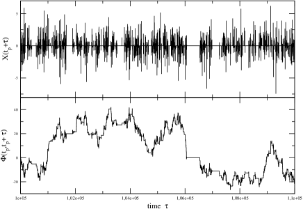
Figure 3: A configuration of the noise $X(t_{p}+\tau)$ in our model (as a function of $\tau$) between $t_{p}=10^{5}\tau_{0}$ and $t_{p}+\tau=1.1~{}10^{5}\tau_{0}$. In this figure, $h=0$ and the waiting times are distributed with an algebraic distribution $P(\tau_{i})\simeq\tau_{i}^{-2.1}$. The bottom part of the figure shows the corresponding continuous time random walk of the accumulated phase of the TLS between $t_{p}$ and $t_{p}+\tau$.

III Dephasing, continuous time random walk of the phase and renewal theory

III.1 Continuous time random walk of the phase

Having defined our model for the intermittent noise field $X(t)$, we will now study its effects on the dephasing of the two-level system, characterized by the dephasing factor (5). Note that a priori this dephasing has several origins : the randomness of the pulses amplitudes $x_{i}$, and the randomness of the waiting times $\tau_{i}$. These two dephasing sources are assumed to be independent from each other in this work. For clarity and pedagogical reasons, we first start by considering the effect of randomness of the pulse amplitudes before turning to the the effect of waiting time randomness.

III.1.1 Dephasing by random phase pulses : the random walk of the phase

Here, we assume that all waiting times are equal $\tau_{i}=t_{i}-t_{i-1}=\tilde{\tau}$. In this case, the phase $\Phi(t_{p},t)$ accumulated between $t_{p}$ and $t_{p}+t$ performs a usual random walk characterized by the distribution $p(x)$ of phase pulses : at the dates $t_{n}=n\tilde{\tau}$, $\Phi(t_{p},t)$ is increased by a random value $x_{i}$. In the limit $|x|\ll 1$, the phase slowly diffuses and dephasing is achieved only after a large number of pulses $n=t_{n}/\tilde{\tau}$. Then, the distribution of the phase $\Phi(t_{p},t_{n})$ can be well approximated by a Gaussian distribution (apart from some irrelevant tails) and the dephasing factor is easily computed. It decays exponentially with characteristic time $\tau_{\phi}=\frac{2\tilde{\tau}}{g^{2}-h^{2}}$.

Note that this diffusive regime can also be studied when the distribution $p(x)$ lacks a finite second or even first moment. An anomalous diffusion of the phase is expectedBouchaud1990 . Let us assume that $x_{i}=h+\kappa\xi_{i}$ where the probability distribution of $\xi_{i}$ has zero average and belongs to the attraction bassin of the stable law $L_{\nu,\beta}$ characterized by the exponent $0<\nu<2$ of the algebraic tails for large values of $\xi_{i}$ and the asymmetry parameter $|\beta|\leq 1$. Then, according to the generalized central limit theorem, the accumulated phase after $n$ pulses is $\Phi_{n}=nh+\kappa\,n^{1/\nu}\xi$ where $\xi$ is distributed according to $L_{\nu,\beta}$. Consequently, in the diffusive limit ($n\ll 1$), the dephasing factor is the product of the homogenous phase $e^{iht/\tilde{\tau}}$ by the characteristic function of $L_{\nu,\beta}$ evaluated for $k\simeq g(t/\tilde{\tau})^{1/\nu}$. For $\nu<2$ and $\nu\neq 1$, this leads to:

$$D_{t_{p}}(t)=e^{-C\kappa^{\nu}t/\tilde{\tau}}\,e^{i(h-C\beta\tan{(\pi\nu/2)}\kappa^{\nu})\,t/\tilde{\tau}}\,.$$ (21)

where $C$ is a numerical constant which can be absorbed in a rescaling of $\kappa$. Thus, in this case, the decay is still exponential and stationary although non Gaussian features of the noise lead to an anomalous dependance of the dephasing time on the coupling constant $\kappa$ that characterizes the scale of the fluctuations of phase pulsesLutz2002 .

III.1.2 Dephasing by random waiting times and continuous time random walk

Let us now turn to the situation where the phase pulses happen at random times. In this case, the accumulated relative phase $\Phi(t_{p},\tau)$ (see eq.(2)) does not perform a random walk as $\tau$ increases, but rather a continuous time random walkMontroll1965 ; Haus1987 (CTRW) on the unit circle. In other words, after some random waiting time $\tau_{i}$, $\Phi(t_{p},\tau)$ is incremented by a random value $x_{i}$ (see figure 3). Thus, on a technical level, the dephasing properties of the two level system are now related to some correlation function of the corresponding CTRW. The corresponding dephasing factor can differ from results obtained in the previous section due to the additional source of dephasing given by the randomness of waiting times. To illustrate this point, let us consider the case where all phase pulses have the same intensity $p(x)=\delta(x-h)$. The accumulated phase after $N$ events is exactly $Nh$. Thus, dephasing comes only from the randomness of the number $N[t_{p},t_{p}+t]$ of events occurring between $t_{p}$ and $t_{p}+t$ and the phase diffusion is governed by the probability distribution for $N[t_{p},t_{p}+t]$. The time needed to obtain $N$ events is the sum over the $N$ first waiting times after $t_{p}$: $t_{N}=\sum_{j=1}^{N}\tau_{j}$. At $t_{p}=0$, all $\tau_{i}$s are distributed according to the same probability distribution and therefore, in the limit of large $N$, the generalized central limit theoremBouchaud1990 can be used (the case $t_{p}\neq 0$ will be discussed below). It provides the limit law for $t_{N}$ at large $N$ which in turn determines the probability law for the number of events. According to this theorem, three classes must be considered depending on whether the moments (9) are finite:

1. The case $\mu>2$ where both $\langle\tau\rangle$ and $\langle\tau^{2}\rangle$ are finite. In this case, the probability distribution for the number of events is gaussian with a vanishing relative uncertainty.

2. The case $1<\mu<2$ where the average of $\tau$ is finite but the second moment diverges.

3. The case $\mu<1$ where all moments diverge.

The usual model for telegraphic noise assumes a Poissonian distribution for the number of events in a given time interval and corresponds to $\psi(\tau)=\gamma e^{-\gamma\tau}$. We will refer it as the Poissonian case and it belongs to the $\mu>2$ class.

Note that non trivial behavior is expected in the last two cases where $\psi$ has infinite first or second moments. In particular, for $\mu<1$, as $\psi(\tau)$ does not have any average, no time scale characterizes the evolution of the noise and, as we will see, nonstationarity follows. This case deserves a special attention as we showed that a $1/f$ spectrum is found precisely for $\mu\to 1$. Before turning to the general formal expressions for the dephasing factor, we will focus on the origin of this nonstationarity.

III.1.3 Origin of the non-stationarity in CTRW : the first waiting time distribution.

Within our model, the waiting times between successive pulses are chosen independently according to the distribution $\psi$. Consequently, all the $t_{p}$ dependence of $\Phi(t_{p},t)$ will come from the choice of $\tau_{1}$ defined as the waiting time between $t_{p}$ and the first spike that follows $t_{p}$ (see figure 4).

Figure 4: Intermittent noise between $t_{p}$ and $t_{p}+t$

Indeed, at time $t_{p}+\tau_{1}$, the CTRW starts anew: $\tau_{2}$ is chosen without any correlation to the history of the CTRW. Hence given the probability distribution of $\tau_{1}$, we can forget about the history of the CTRW of the phase and describe its behavior starting at $t_{p}$. This remark is at the core of the use of renewal theory. In the following, the probability distribution of $\tau_{1}$ will be denoted by $\psi_{t_{p}}$ and a priori, it may depend on $t_{p}$. In fact, as we shall see later, its behavior can be quite counter-intuitive.

First of all, note that a given $\tau_{1}$ can be obtained from many different noise configurations that differ from the time of the last event occurring before $t_{p}$. Separating noise configurations (starting at $t=0$) that have their first spike at time $t_{p}+\tau_{1}$ from the others leads to an integral equation that determines $\psi_{t_{p}}$ in terms of $\psi$ ($S$ is determined from $\psi$ through an integral equation (45)):

$$\psi_{t_{p}}(\tau_{1})=\psi(t_{p}+\tau_{1})+\int_{0}^{t_{p}}d\tau~{}\psi(\tau_{1}+\tau)S(t_{p}-\tau)\,.$$ (22)

The integral in the r.h.s. comes from noise configurations that have a spike between $0$ and $t_{p}$. Equation (22) is the starting point for deriving analytic results about $\psi_{t_{p}}$ in appendix B and C using Laplace transform techniques. Before computing exactly the dephasing factor, let us show some of the counter-intuitive properties of $\psi_{t_{p}}(\tau_{1})$. In particular from (22), we can derive the following expression for the average of $\tau_{1}$ valid for $\mu>2$:

$$\langle\tau_{1}\rangle_{\psi_{t_{p}}}=\frac{\langle\tau^{2}\rangle}{2\,\langle\tau\rangle}=\frac{\langle\tau\rangle}{2}+\frac{\langle\tau^{2}\rangle-\langle\tau\rangle^{2}}{2\,\langle\tau\rangle}.$$ (23)

This first term corresponds to the case of regularly spaced pulses averaged over the origin of times. The second term is the contribution of fluctuations. This result means that irregularities in the event spacings increase the average waiting time of the first event following $t_{p}$. The r.h.s. of (23) does not depend on $t_{p}$, as expected from the stationarity of the CTRW for $\mu>2$ after a short transient regime at small $t_{p}$. On the other hand, for $\mu<2$, eq. (23) is expected to break down since $\langle\tau^{2}\rangle$ diverges. This divergence signals that in some noise configurations $\tau_{1}$ can become of the order of $t_{p}$ and, as a consequence, the average properties of the CTRW after $t_{p}$, depend on this age of the noise. Indeed, we can show from (22) that $\langle\tau_{1}\rangle_{\psi_{t_{p}}}$ scales with the age as $t_{p}^{2-\mu}$. Note that in the diffusion regime, many phase pulses are necessary to dephase the qubit. Therefore, we expect that, in this regime, the aging effect on $\psi_{t_{p}}(\tau_{1})$ only brings weak corrections to the dephasing scenario as will be confirmed below by exact computations. However, we shall see in the following that the $t_{p}$ dependence of $\psi_{t_{p}}$ for $\mu\leq 1$ has much more spectacular consequences on the dephasing factor than in the $1<\mu<2$.

We will now show that, knowing the Laplace transform of $\psi_{t_{p}}$, an explicit expression for the Laplace transform of the average dephasing factor can be obtained.

III.2 Exact dephasing via renewal theory

III.2.1 Dephasing factor

Among all noise configurations that are to be taken into account, some of them (possibly very few) do not have any event between $t_{p}$ and $t_{p}+t$. Their total weight is given by $\Pi_{0}(t_{p},t)$ which is

$$\Pi_{0}(t_{p},t)=\int_{t}^{+\infty}\psi_{t_{p}}(\tau)\,d\tau.$$ (24)

All other histories have at least one event between $t_{p}$ and $t_{p}+t$. Let us assume that it happens at $t_{p}+\tau$ where $\tau$ lies between $0$ and $t$. Then after this event, the noise starts anew. The jump itself contributes by $\overline{e^{ix}}$ to the dephasing factor and the rest of the noise configuration contributes by $D_{0}(t-\tau)$ (i.e. $t_{p}=0$ in eq.(5)). The probability that the first event after $t_{p}$ happens at time $t_{p}+\tau$ is nothing but $\psi_{t_{p}}(\tau)$. Hence the contributions to $D_{t_{p}}(t)$ from all possible noise configurations take the form of the following renewal equation:

$$D_{t_{p}}(t)=\Pi_{0}(t_{p},t)+\overline{e^{ix}}\,\int_{0}^{t}\psi_{t_{p}}(\tau)D_{0}(t-\tau)\,d\tau.$$ (25)

Note that the Laplace transform of this expression is very simple:

$$L[D_{t_{p}}]=L[\Pi_{0}]+(1-f)\left(L[\psi_{t_{p}}]\ldotp L[D_{0}]\right).$$ (26)

where $f=1-\overline{e^{ix}}$. Specializing $t_{p}=0$, one gets an expression for $D_{0}(t)$ that contains $\Pi_{0}(0,t)$. Since $\Pi_{0}(0,t)=\int_{t}^{\infty}\psi(\tau)\,d\tau$ an explicit expression for the Laplace transform of $D_{0}$ can be found:

$$L[D_{0}]=\frac{1}{s}\,\frac{1-L[\psi]}{1-(1-f)\,L[\psi]}.$$ (27)

Plugging expression (27) into equation (26) gives:

$$L[D_{t_{p}}]=\frac{1}{s}\left(1-\frac{f\,L[\psi_{t_{p}}]}{1-(1-f)L[\psi]}\right)\,.$$ (28)

This exact expression will be extensively used to derive both analytic expressions and numerical plots by Laplace inversion. Before proceeding along, let us express $L[D_{t_{p}}]$ in terms of the density of events. It is then convenient to define $S_{t_{p}}(t)=S(t_{p}+t)$ (see appendix A). From the expressions in this appendix of $L[S_{t_{p}}]$ and $L[S]$ in terms of $L[\psi]$ and $L[\psi_{t_{p}}]$, we obtain

$$L[D_{t_{p}}]=\frac{1}{s}\left(1-\frac{f\,L[S_{t_{p}}]}{1+f\,L[S]}\right).$$ (29)

Equation (28) and (29) enable analytical estimates of the dephasing factor in various limiting regimes. Equation (29) is useful in the limit of small coupling (i.e. $f\rightarrow 0$) whereas eq. (28) will be useful in the opposite limit of a wide distribution of spikes’ heights (i.e. $f\rightarrow 1$).

III.2.2 Weak and strong coupling regimes

In the limit of very strong coupling ($f=1$), the phase spreading of a single spike is sufficient to dephase the qubit. In this case, eq.(25) immediately leads to $D_{t_{p}}(t)=\Pi_{0}(t_{p},t)$. This means that the whole average is dominated by the rare noise configurations that do not evolve during the experiment. As we shall see later, this leads to a strong $t_{p}$ dependence of $D_{t_{p}}(t)$ for $\mu<2$.

At much lower couplings ($|f|\ll 1$), it is not a priori clear whether the renewal equation for $D_{t_{p}}(t)$ induces a strong dependence of $D_{t_{p}}(t)$ on $t_{p}$. Pushing the above analysis forward amounts to compare the time dependence of the two terms in the r.h.s. of the renewal equation (25). As we will see now, it will provide a better understanding of the physics underlying the dephasing scenario.

Let us first assume that $\Pi_{0}(t_{p},t)$ decays much faster than $D_{0}(t)$. Since $\psi_{t_{p}}(\tau)=-\partial_{\tau}\Pi_{0}(t_{p},\tau)$, it also decays much faster than $D_{0}$. Consequently, we can approximate $\psi_{t_{p}}(\tau)D_{0}(t-\tau)$ by $\psi_{t_{p}}(\tau)D_{0}(t)$ in Eq.(25). Then, after a short initial decay due to both $D_{0}(t)$ and $\Pi_{0}(t_{p},t)$, $D_{t_{p}}(t)$ decays as $D_{0}(t)$. Consequently, the dephasing time does not depend on $t_{p}$. For instance, we expect this situation to occur at weak coupling when the average waiting time $\langle\tau\rangle$ is finite since the probability that no event occurs between $t_{p}$ and $t_{p}+t$ vanishes quite fast when $t$ increases. Note that in the limit of vanishing coupling, the spreading of the phase can become much slower than the decay of $\Pi_{0}(t_{p},t)$ and thus our starting point hypothesis is valid.

The opposite case where the decay of $D_{0}(t)$ is much faster than the decay of $\Pi_{0}(t_{p},t)$ can be discussed more conveniently by integrating the renewal equation (25) by parts. Considering again $g\ll 1$ we get:

$$D_{t_{p}}(t)\simeq D_{0}(t)-\int_{0}^{t}\Pi_{0}(t_{p},t-\tau)D^{\prime}_{0}(\tau)\,d\tau\,.$$ (30)

Approximating $\Pi_{0}(t_{p},t-\tau)\approx\Pi_{0}(t_{p},t)$ in this equation yields $D_{t_{p}}(t)=D_{0}(t)+\Pi_{0}(t_{p},t)(1-D_{0}(t))$. As a consequence, once $D_{0}(t)$ has decayed, the dephasing factor is almost equal to $\Pi_{0}(t_{p},t)$. This is the same behavior than in the very strong coupling regime $f=1$, although here, we assumed $|f|\ll 1$. This regime is expected to occur when the decaying time scales of $D_{0}(t)$ and of $\Pi_{0}(t_{p},t)$ are comparable. This is obviously the case at very strong coupling but, surprisingly, as we shall see now it can also be obtained for $|f|\ll 1$!

First of all, the above discussion shows that such a regime can only happen if the average waiting time is infinite, i.e. for $\mu<1$. In this case, $\Pi_{0}(t_{p},t)$ can be evaluated analytically (see eq. (82)): it is shown to be independent of $\tau_{0}$ and to exhibit aging behavior (i.e. to depend only on $t/t_{p}$). Therefore, the decaying time scale of $\Pi_{0}(t_{p},t)$ scales as $t_{p}$. Comparing this time scale with the dephasing time scale for $|f|\ll 1$, leads to a $t_{p}$ dependent cross-over coupling constant $f_{c}(t_{p})$. In the case of aging $\Pi_{0}$, the crossover coupling decays to lower and lower values by increasing $t_{p}$.

For $|f|\gtrsim f_{c}(t_{p})$, the dephasing factor behaves as $\Pi_{0}(t_{p},t)$ and the dephasing time saturates as a function of $f$. Such a saturation of the dephasing time as a function of the amplitude of the noise has already been discussed for a Poissonian fluctuatorFalci2003 ; Galperin2003 . In this case $\Pi_{0}(t_{p},t)=\Pi_{0}(0,t)=e^{-t/\langle\tau\rangle}$ decays very fast, on a time scale $\langle\tau\rangle$. The cross-over between weak and strong coupling regime happens precisely at the point where the dephasing time assuming weak coupling $\langle\tau\rangle/g^{2}$ is of the same order as this decay time, i.e. for $g\sim 1$. Note that in this case, as expected from our discussion, the crossover scale is independent of the age of the noise $t_{p}$. We expect this reasoning to break down in our model because of the broad distribution of waiting times ($\mu<2)$. Understanding the various dephasing scenarii and computing the $t_{p}$ dependence of the crossover coupling in our case requires the computation of $\Pi_{0}(t_{p},t)$ and of $D_{0}(t)$. These quantitative results will be presented in forthcoming sections.

To summarize the above discussion, we have argued that the dephasing time is bounded by the typical decay time of both $\Pi_{0}(t_{p},t)$ and $D_{0}(t)$. This suggests to distinguish between two regimes: on one hand, a weak coupling regime for which $D_{0}(t)$ decays much slower than $\Pi_{0}(t_{p},t)$ and for which the dephasing time - in that case just the decay time of $D_{0}(t)$ - is not sensitive to $t_{p}$. On the other hand, a strong coupling regime for which $D_{0}(t)$ decays faster than $\Pi_{0}(t_{p},t)$. In that case, the dephasing time is given by the decay time of $\Pi_{0}(t_{p},t)$ and thus possibly $t_{p}$-dependent. As the above discussion shows, the cross-over between these two regimes may happen for a possibly $t_{p}$ dependent cross-over coupling $f_{c}(t_{p})\ll 1$. Note that in the strong coupling regime, the dephasing time becomes independent of the amplitude of the noise whereas in the weak coupling regime, it is expected to depend on the amplitude and to diverge in the vanishing coupling limit.

IV Dephasing in the symmetric models

In this section we present our results for the situation of a symmetric distribution of the spikes, $p(-x)=p(x)$. Under this assumption the average random accumulated phase vanishes, i.e. $f$ and consequently $D_{t_{p}}(t)$ are real. For $g\ll 1$, $f$ may be expanded in moments of $p(x)$, $f\approx g^{2}\ll 1$ where $g$ measures the typical scale of the fluctuations of the spikes.

IV.1 Dephasing at $t_{p}=0$

Before discussing the decoherence factor for arbitrary preparation time $t_{p}$, it is useful to investigate the case $t_{p}=0$. Rewriting the Laplace transform of $D_{0}(t)$ (27) as

$$L[D_{0}](s)=\frac{1}{s}\left(1+\frac{fL[\psi]}{1-L[\psi]}\right)^{-1}$$ (31)

suggests to introduce a scale $\gamma_{g}$ related to the strength of the coupling:

$$\left.\frac{fL[\psi]}{1-L[\psi]}\right|_{s=\gamma_{g}}=1\,.$$ (32)

Note that $\gamma_{g}$ vanishes with the coupling $g$. Investigating the behavior of $D_{0}$ for $t\ll\tau_{0}$ requires evaluating the Laplace transform for $s\tau_{0}\ll 1$. In this regime, the Laplace transform $L[\psi]/(1-L[\psi])$ can be approximated by $1/(1-L[\psi])$. Within this approximation, we shall now derive explicit expressions for $L[D_{0}]$ which can be Laplace inverted explicitly. This leads to expressions for $D_{0}(t)$ valid at $t\gg\tau_{0}$ for the different classes of $\mu$.

In the case of finite average waiting time ($\mu>1$), we can expand $L[\psi]\approx 1-s\langle\tau\rangle$ to find the leading contribution to $D_{0}(t)$ for $\langle\tau\rangle\ll\gamma_{g}t<1$. This gives:

$$D_{0}(t)\simeq L^{-1}\left[\frac{\langle\tau\rangle}{s\langle\tau\rangle+f}\right]=e^{-t/\tau_{\phi}}\;,$$ (33)

with the dephasing time $\tau_{\phi}=\gamma_{g}^{-1}=\langle\tau\rangle/f$ (see eq. (32)). Note that this expression is exact only for $\psi(\tau)=\frac{1}{\langle\tau\rangle}e^{-\tau/\langle\tau\rangle}$. At finite non integer $\mu$, taking into account the fluctuations of the waiting times requires keeping all terms in $1-L[\psi]$ up to the first non integer power $(s\tau_{b})^{\mu}$. For $1<\mu<2$, we get algebraic subleading corrections to (33): $\log{(D_{0}(t))}\simeq-\gamma_{g}t-fc(\mu)(t/\tau_{0})^{2-\mu}$, where $c(\mu)=(\mu-1)/(2-\mu)$. These corrections being weak for $g\ll 1$, the dephasing time $\tau_{\phi}$ remains equal to $\gamma_{g}^{-1}=\langle\tau\rangle/g^{2}$ in this regime.

For $\mu<1$, the first term in the expansion of $1-L[\psi]$ is proportional to $(\tau_{0}s)^{\mu}$. Therefore, plugging in $(1-L[\psi])/L[\psi]\simeq\Gamma(1-\mu)(s\tau_{0})^{\mu}$ and performing the inverse Laplace transform of (31) gives:

$$D_{0}(t)\simeq L^{-1}\left[\frac{s^{-1}}{1+f(s\tau_{0})^{-\mu}}\right]=E_{\mu}\left[-\left(\gamma_{g}t\right)^{\mu}\right]$$ (34)

where $E_{\mu}(z)=\sum_{n=0}^{\infty}\frac{z^{n}}{\Gamma(1+\mu n)}$ denotes the Mittag-Leffler functionBateman1955 . For values of $\mu$ close to one and $z\lesssim 1$ this function can be approximated by a simple exponential, whereas for $\mu\sim 0$ it is similar to an algebraic function $E_{\mu}(z)\sim(1+z)^{-1}$. For large values of the argument ($\left|z\right|\gg 1$) and $\left|\mathrm{arg}(-z)\right|<(1-\mu/2)\pi$, we obtainBateman1955 $E_{\mu}(z)\approx(-z\Gamma(1-\mu))^{-1}$. This change of behavior from an exponential to an algebraic behavior was interpreted in ref. Schriefl2004, as a Griffith effect.

Computing long time behavior ($\gamma_{g}t\gg 1$) of the dephasing factor can be done by expanding (31) as follows:

$$L[D_{0}](s)\simeq\frac{1}{s}\frac{1-L[\psi]}{fL[\psi]}\;.$$ (35)

For $\gamma_{g}t\gg 1$ ($s\ll\gamma_{g}$) we can safely replace $L[\psi]\approx 1$ in the denominator. The inverse Laplace transform can then be done easily and reads for $\gamma_{g}t\gg 1$ :

$$D_{0}(t)\simeq\frac{1}{f}\int_{t}^{\infty}\psi(\tau)\,d\tau=\frac{1}{f}\left(\frac{\tau_{0}}{\tau_{0}+t}\right)^{\mu}\;.$$ (36)

For $\mu<1$, (36) is nothing but the asymptotic behavior of (34) for $\gamma_{g}t\gg 1$. Note that for $g\gg 1$, $\gamma_{g}^{-1}$ is of the order of $\tau_{0}$ and the decay is algebraic at all times $t>\tau_{0}$, given by (36). For $1<\mu<2$ and $g\ll 1$, only at large times ($\gamma_{g}t\sim\ln(1/f)$), when the qubit has almost completely dephased, the decay crosses over to the power law (36).

IV.2 Influence of a finite preparation time $t_{p}$

We will now discuss in detail the $t_{p}$-dependence of the dephasing scenario and of the crossover coupling strength $g_{c}$ for the different classes of $\mu$. Simple analytical expressions for $D_{t_{p}}(t)$ can be derived in the weak $(g\ll g_{c})$ and strong $(g\gg g_{c})$ coupling regimes.

IV.2.1 Infinite fluctuations of the waiting times: $1<\mu<2$

For $1<\mu<2$, the decay of $D_{0}(t)$ is accurately described by (33) and (36). On the other hand, $\Pi_{0}(t_{p},t)$ exhibits an explicit dependence on the age of the noise (see appendix D):

$$\Pi_{0}(t_{p},t)\simeq\left(\frac{\tau_{0}}{\tau_{0}+t}\right)^{\mu-1}-\left(\frac{\tau_{0}}{\tau_{0}+t+t_{p}}\right)^{\mu-1}$$ (37)

for $t_{p}\gg\tau_{0}$. We will arbitrarily define the typical time scale of the decay of any function as the time at which its modulus reaches a fixed value $0<\alpha<1$ ($\alpha=1/e$ in all the figures of this paper). The cross-over between a weak and strong coupling regime is defined as the value of $g$ where the typical decay times of $D_{0}(t)$ and $\Pi_{0}(t_{p},t)$ coincide (see section III.2.2). In the present case, the cross-over coupling gets a weak $t_{p}$ dependence:

$$(g_{c}(t_{p}))^{2}\simeq\frac{1}{\mu-1}\left[\alpha+\left(\frac{\tau_{0}}{t_{p}}\right)^{\mu-1}\right]^{1/(\mu-1)}\;.$$ (38)

Note that $g_{c}$ is a decreasing function of $t_{p}$ since increasing $t_{p}$ slows down the decay of $\Pi_{0}(t_{p},t)$ (remember that the average time of the first occurring spike after $t_{p}$ increases as $t_{p}^{2-\mu}$). But since the average waiting time is finite, $g_{c}$ has a non zero lower bound. Note also that the $t_{p}$-dependence of $g_{c}$ is only visible for values of $\mu$ close to one and disappears as $\mu$ increases to higher values. This can be seen on the numerical results depicted on fig. 6: $g_{c}(t_{p})$ is the crossover coupling where the dephasing time start to saturate as a function of $g$.

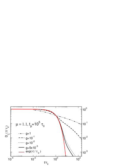
Figure 5: Dephasing factor $D_{t_{p}}(t)$ in the symmetric model obtained by numerical Laplace inversion for $\mu=1.1$ and $t_{p}=10^{5}$ and various values of $g$. At small couplings, the decay is exponential. But at longer times $t\gg\tau_{\phi}$ and for strong coupling the decay is algebraic.

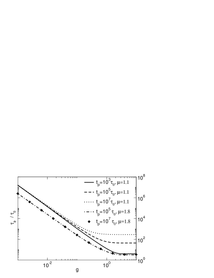
Figure 6: Dephasing time $\tau_{\phi}$ in the symmetric model as a function of $g$ for $\mu=1.1$, $\mu=1.8$ and for various values of $t_{p}$. At strong coupling the dephasing time exhibits $t_{\mathrm{p}}$-dependence, which disappears as $\mu$ increases to higher values. Note that the critical coupling $g_{c}$ has a weak $t_{\mathrm{p}}$-dependence for $\mu$ close to one.

In the case of very strong coupling ($g\gg g_{c}(t_{p})$), the decay of $D_{t_{p}}(t)$ coincides with $\Pi_{0}(t_{p},t)$ and is thus algebraic at all times (see fig. 5). On the other hand, at weak coupling ($g\ll g_{c}$), the dephasing factor $D_{t_{p}}(t)$ follows $D_{0}(t)$ up to times of the order of the dephasing time, i.e. it decays exponentially: $D_{t_{p}}(t)=\exp(-t/\tau_{\phi})$, where $\tau_{\phi}=\gamma_{g}^{-1}=\tau_{0}g^{-2}$. In this weak coupling regime, the dephasing is thus described accurately using a second cumulant expansion. However, for times large compared to the dephasing time, $t\gtrsim\tau_{\phi}\ln(\tau_{\phi}/\tau_{0})$, higher cumulants contribute and the decay goes over to a much slower power law. If $t_{p}<\tau_{\phi}$ the asymptotic decay of $D_{t_{p}}(t)$ continues to follow $D_{0}(t)$ behavior given in (36) whereas, in the opposite case $t_{p}>\tau_{\phi}$ it is given by $\Pi_{0}(t_{p},t)$ (37).

IV.2.2 Infinite average waiting time: $0<\mu<1$

For $0<\mu<1$ the influence of a finite preparation time $t_{p}$ becomes even more drastic, due to the absence of a characteristic time scale in the waiting time distribution. In this case $\Pi_{0}(t_{p},t)$ only depends on the ratio $t/t_{p}$ (aging behavior):

$$\Pi_{0}(t_{p},t)=\frac{\sin{(\pi\mu)}}{\pi\mu}\,\left(\frac{t_{p}}{t}\right)^{\mu}\,{}_{2}F_{1}(1,\mu;1+\mu;-\frac{t_{p}}{t})\;,$$ (39)

where ${}_{2}F_{1}$ denotes a hypergeometric functionGradsteyn1980 . Consequently, the typical decay time of $\Pi_{0}(t_{p},t)$ is proportional to $t_{p}$. On the other hand, $D_{0}(t)$ is given by (34) and its decay time thus scales as $\tau_{\phi}=\gamma_{g}^{-1}\propto\tau_{0}/f^{1/\mu}\approx\tau_{0}/g^{2/\mu}$ in the limit $g\ll 1$. As a consequence, the crossover coupling strength $g_{c}$ exhibits a strong $t_{p}$ dependence:

$$g_{c}(t_{p})=\lambda(\mu)\left(\frac{\tau_{0}}{t_{p}}\right)^{\mu/2}\ll 1\,,$$ (40)

where $\lambda(\mu)$ is a function of $\mu$ that can be obtained by inversion of (39) and (34). As in the case $1<\mu<2$, $g_{c}$ is a decreasing function of $t_{p}$: the range of the strong coupling regime increases with the age of the noise. However, contrarily to the case $1<\mu<2$, $g_{c}$ has no lower bound, i.e. it decays to zero as we increase $t_{p}$. Consequently, any qubit surrounded by a noise with $0<\mu<1$ will eventually end up in the strong coupling regime. This can be seen on results depicted on figure 7.

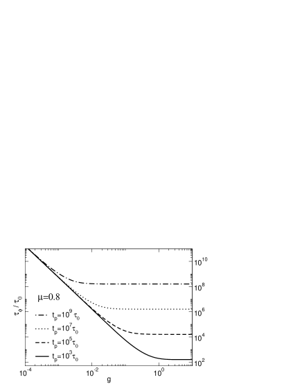
Figure 7: Dephasing time $\tau_{\phi}$ in the symmetric model as a function of $g$ for $\mu<1$ and for various values of $t_{p}$. At strong coupling the dephasing time exhibits a $t_{\mathrm{p}}$-dependence, which disappears as $\mu$ increases to higher values. Note the explicit $t_{\mathrm{p}}$-dependence of the critical coupling $g_{c}$.

At strong coupling ($g>g_{c}(t_{p})$), $D_{t_{p}}(t)$ is given by $\Pi_{0}(t_{p},t)$ and therefore is only a function of $t/t_{p}$. In this regime, the dephasing time is proportional to $t_{p}$, as shown on fig. 8. The initial decay of coherence is quite fast since, for $t\ll t_{p}$, $\Pi_{0}(t_{p},t)\approx 1-A(\mu)(t/t_{p})^{1-\mu}$ with $A(\mu)=\sin(\pi\mu)/[(1-\mu)\pi]$. Consequently, for $\mu$ close to one $D_{t_{p}}(t)$ decays substantially for times short compared to the preparation time $t_{p}$. For $t\gtrsim t_{p}$, the decay slows down considerably and goes over to a power law $\Pi_{0}(t_{p},t)\propto(t_{p}/t)^{\mu}$.

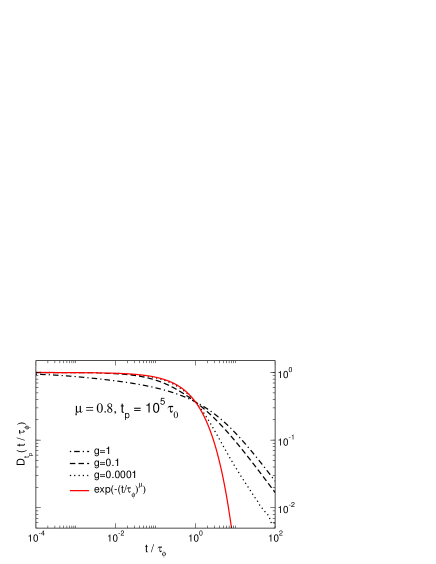
Figure 8: Dephasing factor $D_{t_{p}}(t)$ in the symmetric model obtained by numerical Laplace inversion for $\mu=0.8$, $t_{p}=10^{5}$ and various values of $g$. For weak coupling, $g<g_{c}(t_{\mathrm{p}})$, the decay is exponential for $t<\tau_{\phi}$. For times $t\gtrsim\tau_{\phi}$ at weak coupling and for strong coupling the decay is algebraic.

At weak coupling ($g<g_{c}(t_{p})$), the decay of $D_{t_{p}}(t)$ is accurately described by (34). For $\mu$ close to 1 and $\gamma_{g}t<1$, the Mittag-Leffler function can be approximated by a exponential decay $D_{t_{p}}(t)\approx\exp[-(\gamma_{g}t)^{\mu}]$, whereas for $0<\mu\ll 1$ and $\gamma_{g}t\lesssim 1$, the decay is rather algebraic, $D_{t_{p}}(t)\approx[1+(\gamma_{g}t)^{\mu}]^{-1}$. In any case, the typical decay time scales as $\tau_{\phi}=\gamma_{g}^{-1}\propto g^{-2/\mu}$. As for $1<\mu<2$, this dephasing time can be recovered using a second cumulant expansion of the phase. Obviously, for larger times, $t>\tau_{\phi}$, higher cumulants contribute and the decay goes over to a power law, $D_{t_{p}}(t)\propto(\tau_{0}/t)^{\mu}$, as shown in Fig (8).

IV.2.3 On the marginal case: $\mu=1$

Finally, in the marginal case $\mu=1$ corresponding to $1/f$ noise, the above analysis is confirmed qualitatively. We mainly find logarithmic corrections to the above results, leading to behaviors intermediate between the classes $\mu<1$ and $1<\mu<2$. The crossover coupling $g_{c}$ in this case turns out to be

$$g_{c}(t_{p})=\left(\frac{\tau_{0}}{t_{p}}\ln(t_{p}/\tau_{0})\right)^{1/2}\,,$$ (41)

showing a strong dependence on the preparation time $t_{p}$. As in the case $\mu<1$, it decays to zero for $t_{p}\to\infty$.

Computing $D_{0}(t)$ requires to invert (31). This cannot be done exactly because of the complicated form of $L[\psi]\simeq 1-s\tau_{0}\left|\ln(s\tau_{0})\right|$ for $s\tau_{0}\ll 1$. However, $D_{0}(t)$ may be estimated considering $\ln{(s\tau_{0})}$ as a constant and replacing $s$ by $1/t$ in its argument. This leads to:

$$D_{0}(t)\simeq\exp\left(-f\frac{t/\tau_{0}}{\ln(t/\tau_{0})}\right)\quad\mathrm{for}\ t\lesssim\frac{\tau_{0}}{f}\left|\ln f\right|\;.$$ (42)

Hence, for weak coupling, $D_{t_{p}}(t)$ decays due to the contribution of $D_{0}(t)$ on a characteristic time scale $\tau_{\phi}\simeq(\tau_{0}/f)\left|\ln f\right|$. Again, for times large compared to the dephasing time, the decay slows down considerably and goes over to a power law (36), $D_{t_{p}}(t)\propto t^{-1}$.

At strong coupling ($g>g_{c}(t_{p})$), $D_{t_{p}}(t)$ follows $\Pi_{0}(t_{p},t)$, which reads in the present case:

$$\Pi_{0}(t_{p},t)\simeq\frac{1}{\ln(1+t_{p}/\tau_{0})}\ln\left(1+\frac{t_{p}}{\tau_{0}+t}\right)\;.$$ (43)

Consequently, the dephasing time exhibits a strong dependence on the preparation time $t_{p}$. However, since $\Pi_{0}(t_{p},t)$ is not a function of $t/t_{p}$ the dephasing time does not scale linearly with $t_{p}$ (as for $\mu<1$) but has a weaker $t_{p}$ dependence which depends on the parameter $\alpha$ used to define $\tau_{\phi}$ ($D_{t_{p}}(\tau_{\phi})=\alpha$).

V Dephasing in the asymmetric models

In this section, we consider asymmetric distributions $p(x)$ of the pulse amplitudes with a non vanishing average $h=\overline{x}$. This obviously corresponds to the generic case for our intermittent noise, but it also appears naturally in the context of decoherence at optimal points discussed in section II.3.

Similar expansions of the exact expression (28) can be performed to derive the detailed decay of $D_{t_{p}}(t)$ in the case of a finite mean value of the noise, $\overline{x}\neq 0$. Nevertheless, analytic expressions are much harder to obtain since in this case $f=1-\overline{e^{ix}}$ is complex. Therefore, in this section, we will mainly derive scaling laws of $\tau_{\phi}$, the critical coupling $g_{c}$ and present numerical computations of $D_{t_{p}}(t)$ in various regimes. Note that at strong coupling, the dephasing is due to single events of the noise, i.e. $D_{t_{p}}(t)\simeq\Pi_{0}(t_{p},t)$. As a consequence, dephasing only depends on $\psi(\tau)$, not on the details of $p(x)$. In this regime, the results reduce to those previously derived for the symmetric case ($h=\overline{x}=0$) in the strong coupling regime. Differences with respect to the symmetric case only arise in the weak coupling regime on which we shall focus in the following.

Before proceeding along, let us recall the notations (7) for the moments of $p(x)$ : $h=\overline{x}$ and $g^{2}=\overline{x^{2}}$. At weak coupling, $f$ may be expanded in moments of $p(x)$: $f\approx-ih+g^{2}/2+\dots$. As expected for $h\ll g^{2}$, the finite mean value does not modify the results of the previous section, i.e. the dominant dephasing is the same as in the $h=0$ case (symmetric noise). However, as $h$ gets of the same order as $g^{2}$ the decay of $D_{t_{p}}(t)$ and the scaling of $\tau_{\phi}$ are modified. Understanding precisely the possibly nonlinear effect of a small bias on the dephasing factor is related to the fluctuation/dissipation issue in CTRW and is out of the scope of the present paper. Therefore we shall now focus on the case of huge asymmetry where $h\gg g^{2}$. In this limiting regime, the pulse dispersion can be forgotten and $h$ is the only coupling parameter. Note that in this specific variant of the asymmetric model, $\Phi_{t_{p}}(t)$ is proportional to the number of events $N[t_{p},t_{p}+t]$ that occur between $t_{p}$ and $t_{p}+t$ and therefore, the dephasing factor as a function of $h$ is the characteristic function of the probability distribution for $N[t_{p},t_{p}+t]$. Contrarily to the case of Poissonian telegraph noisePaladino2002 ; Galperin2003 where a finite mean value of the noise just adds a global phase to $D_{t_{p}}(t)$, we will see that strong fluctuations in the occurrence times of the spikes induce dephasing even for a fixed value of the phase pulses.

V.1 The $0<\mu<1$ class

In the $0<\mu<1$ case, we can use the same method as for the derivation of (34) to find the scaling law of $\tau_{\phi}$ as a function of the coupling strength. The dephasing factor in the weak coupling regime decays as $\left|D_{t_{p}}(t)\right|=\left|E_{\mu}(iz)\right|$ where $z\simeq-h(t/\tau_{0})^{\mu}/\Gamma(1-\mu)$ and $E_{\mu}$ denotes the Mittag-Leffler function previously used. Using the series expansion that defines $E_{\mu}$, it can be shown easily that $\left|E_{\mu}(iz)\right|$ only depends on $z^{2}$. As a consequence, the dephasing time in the weak coupling regime scales as $\tau_{\phi}\propto\tau_{0}/h^{1/\mu}$, as shown in Fig. 9.

The cross-over between weak and strong coupling regime is obtained by comparing this time scale with the typical decay time of $\Pi_{0}(t_{p},t)$, which is proportional to $t_{p}$ for $0<\mu<1$. Therefore the critical coupling strength scales as $h_{c}\propto t_{p}^{-\mu}$.

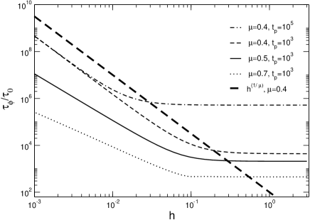
Figure 9: Dephasing time $\tau_{\phi}$ in the asymmetric model as a function of the coupling $g$ for a huge asymmetry $h\gg g^{2}$, and different values of $\mu<1$. At weak coupling, $h<h_{c}(t_{p})$, the dephasing time scales as $\tau_{\phi}\propto 1/h^{1/\mu}$, whereas it becomes proportional to $t_{p}$ for $h>h_{c}(t_{p})$. Note the $t_{p}$-dependence of the critical coupling $h_{c}$, visualized for $\mu=0.4$.

Fig. 10 shows $D_{t_{p}}(t)$ for $\mu=0.8$ and different values of the coupling strength from the weak coupling regime to slightly above $h_{c}$. The initial decay, up to the dephasing time, follows the previous exponential decay. At larger times the decay crosses over to a power law, $D_{t_{p}}(t)\propto 1/t^{\mu}$, as in the symmetric case. Between these two asymptotic behaviors, beatings may occur, due to interferences between different noise histories, as already seen in other models Falci2003 . However, in this reference, oscillations appear in the strong coupling regime. They arise from interferences between noise histories associated with different initial conditions. Such a strong initial condition dependence is expected at strong coupling for a Poissonian fluctuator. In our case, oscillations are also present at $t_{p}=0$ in the diffusion regime and therefore cannot be explained by an initial condition dependence. Nevertheless they are still associated with an interference effect between noise histories.

To illustrate this point, let us mention that for $D_{0}(t)$, a numerical investigation shows that in the situation considered here ($h\gg g^{2}$), these oscillations are only present for $\mu>1/2$. More precisely, the probability distribution for the accumulated phase $\Phi_{0}(t)$ can be computed analytically in the diffusion regime. In this limit $\Phi_{0}(t)=hN[0,t]$ can be viewed as a positive real number. For $0<\mu<1$, its probability distribution is highly non Gaussian and given by

$$P_{0,t}(\phi)=\frac{t}{\mu\,\tau_{\phi}(h)\,\phi^{1+1/\mu}}\,L_{\mu}\left(\frac{t/\tau_{\phi}(h)}{\phi^{1/\mu}}\right)$$ (44)

where $\tau_{\phi}(h)=\tau_{0}\,(\Gamma(1-\mu)/h)^{-1/\mu}$ and $L_{\mu}$ denotes the fully asymmetric Lévy distribution of index $\mu$. For $\mu<1/2$, it decays monotonically whereas for $\mu>1/2$, it grows towards a maximum before decreasing rapidely for large values. This maximum can be viewed as a precursor of the maximum expected for $1<\mu<2$ close the average value $ht/\langle\tau\rangle$ of the phase (for $1<\mu<2$, $P_{0,t}$ is a truncated Lévy distribution whereas for $\mu\geq 2$ it is Gaussian). It is precisely this local maximum that leads to oscillations in the modulus of the dephasing factor.

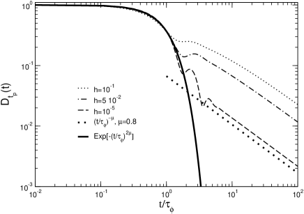
Figure 10: Decay of $\left|D_{t_{p}}(t)\right|$ in the asymmetric model for $\mu=0.8$, $t_{p}=10^{3}\tau_{0}$ and different values of the coupling strength $h$. Here $h_{c}(10^{3}\tau_{0})\simeq 10^{-2.4}$

Note that these oscillations might be related to the Griffith effect mentioned in ref. Schriefl2004, .

V.2 The intermediate class $1<\mu<2$

In the intermediate case of diverging variance, $1<\mu<2$, it is even harder to find scaling laws analytically. Numerically, one finds that the decay time of $D_{t_{p}}(t)$ in the weak coupling regime scales as $\tau_{\phi}\propto\tau_{0}/h$. This leads to a critical coupling $h_{c}(t_{p})$ equal to the r.h.s of (38). At weak coupling, the decay roughly follows an exponential $\exp(-t/\tau_{\phi})$ up to times of the order of $\tau_{\phi}$. At larger times it crosses over to a power law, $D_{t_{p}}(t)\propto 1/t^{\mu}$. Again, at intermediate times and in the weak coupling regime $D_{t_{p}}(t)$ shows a transcient regime. Note also that the cross-over between the weak and strong coupling regimes happens in a much larger ($\mu$-dependent) range of the coupling strength than in the symmetric case.

VI Discussion and conclusion

To conclude, we have proposed a new model for an intermittent classical noise with a $1/f$ power spectrum. Within this model, the noise consists in a succession of pulses, separated by random waiting times. We have shown within this context that the intermittence associated with the $1/f$ characteristics implies a non-stationarity of the noise. Non-stationarity effects are present in some of the regimes of the dephasing of a two level system coupled to this noise as summarized on tables 1 and 2 for the symmetric model. In particular, in the strong coupling regime, the dephasing factor decays algebraically in time, with a characteristic time of decay (dephasing time) depending on the age $t_{p}$ of the noise. On the other hand, in the weak coupling regime an initial exponential decay of this dephasing factor is found. However, for low frequency noises and contrarily to the usual behavior, this exponential is stretched and the dephasing time shows an anomalous dependence on the coupling to the noise. After this initial decay, the dephasing factor decays algebraically. An important observation is that the critical coupling strength separating the weak and strong coupling regimes does depend on the age of the noise when it is non-stationary. More precisely, it decays to zero with the age, such that any qubit coupled to a non-stationary noise will eventually fall in the strong coupling regime.

One should be careful that the dephasing factor that we studied is defined as a configuration average, or ensemble average over the noise (see eq. (5)). In the usual experimental protocols, information on the quantum statistics of the qubit is collected in a given sample in successive runs. This corresponds to a time average in a given configuration. These two averages do not coincide in general for non-stationary or aging phenomena. Indeed, the non-stationarity of the $1/f$ noise that we considered is closely related to the weak ergodicity breaking found in similar trap models for glassy materialsBouchaud1992 . Thus one should be careful in interpreting the non-stationary dephasing factor that we found in some regimes. We nevertheless hope that the questions raised by our results might lead to some possible experimental setup to better characterize the low frequency noise in mesoscopic solids.

Exponent $\mu$	Critical coupling $g_{c}(t_{\mathrm{p}})$	Dephasing time $\tau_{\phi}$
		$g<g_{c}$	$g>g_{c}$
$1<\mu<2$	$g_{c}(t_{\mathrm{p}})^{2}=\frac{1}{\mu-1}\left[\frac{1}{e}+\left(\frac{\tau_{0}}{t_{\mathrm{p}}}\right)^{\mu-1}\right]^{1/(\mu-1)}$	$\tau_{\phi}=\tau_{0}g^{-2}$	$\tau_{\phi}=\tau_{0}[1/e+(\tau_{0}/t_{\mathrm{p}})^{\mu-1}]^{-1/(\mu-1)}$
$\mu=1$	$g_{c}(t_{\mathrm{p}})^{2}=\frac{\tau_{0}}{t_{\mathrm{p}}}\ln\left(t_{\mathrm{p}}/\tau_{0}\right)$	$\tau_{\phi}=\frac{\tau_{0}}{f_{g}}|\ln f_{g}|$	$\tau_{\phi}=\tau_{0}(t_{\mathrm{p}}/\tau_{0})^{1-1/e}$
$0<\mu<1$	$g_{c}(t_{\mathrm{p}})^{2}\propto\left(\frac{\tau_{0}}{t_{\mathrm{p}}}\right)^{\mu}$	$\tau_{\phi}=\tau_{0}g^{-2/\mu}$	$\tau_{\phi}\propto t_{\mathrm{p}}$

Table 1: Critical coupling and dephasing time in the symmetric model for different waiting time distributions.

Exponent $\mu$	$g>g_{\mathrm{c}}$		$g<g_{\mathrm{c}}$
			$t\ll\tau_{\phi}$	$t\gg\tau_{\phi}$
$1<\mu<2$	$\left(\frac{\tau_{0}}{\tau_{0}+t}\right)^{\mu-1}-\left(\frac{\tau_{0}}{\tau_{0}+t_{\mathrm{p}}+t}\right)^{\mu-1}$		$\exp(-t/\tau_{\phi})$	$t_{\mathrm{p}}<\tau_{\phi}:\;\exp(-t/\tau_{\phi})$
				$t_{\mathrm{p}}>\tau_{\phi}:\;\left(\frac{\tau_{0}}{\tau_{0}+t}\right)^{\mu-1}$
$\mu=1$	$\frac{1}{\ln(1+t_{\mathrm{p}}/\tau_{0})}\ln\left(1+\frac{t_{\mathrm{p}}}{\tau_{0}+t}\right)$		$\exp\left(-f_{g}\frac{t/\tau_{0}}{\ln(t/\tau_{0})}\right)$	$1/t$
$0<\mu<1$	$t\ll\tau_{\phi}$	$t\gg\tau_{\phi}$	$\mu\simeq 1:\;\exp[-(t/\tau_{\phi})^{\mu}]$	$\left(\frac{\tau_{0}}{t}\right)^{\mu}$
	$1-A(\mu)(t/t_{\mathrm{p}})^{1-\mu}$	$(t_{\mathrm{p}}/t)^{\mu}$	$\mu\ll 1:\;\frac{1}{1+(t/\tau_{\phi})^{\mu}}$

Table 2: Summary of the different expressions of the decoherence factor $D_{t_{\mathrm{p}}}$ in the symmetric model.

Appendix A Useful results on the sprinkling time distribution

A.1 Definition

This distribution $S(t)$ is defined as the probability density that an event occurs exactly at time (date) $t$. Hence $S(t)$ satisfies the equation

$$S(t)=\psi(t)+\int_{0}^{t}dt^{\prime}\psi(t-t^{\prime})S(t^{\prime})\,,$$ (45)

which states that the spike at $t$ is either the first one, or follows a previous spike at time $t-t^{\prime}$. In Laplace transform, this reads:

$$L[S](s)=\frac{L[\psi](s)}{1-L[\psi](s)}\,.$$ (46)

Whenever $\psi(\tau)$ has a finite mean, $S(t)$ is constant, equal to $1/\langle\tau\rangle$ with possible large fluctuations ($\mu>1$).

A.2 Explicit expressions

In the case of a Poissonian waiting time distribution $\psi(\tau)=\gamma\,e^{-\gamma\tau}$, $S(t)$ is a constant equal to $1/\langle\tau\rangle$ for all times. When $\psi$ has algebraic tails at long times, we expect this result to be modified since the rate of events is expected to decrease with the sampling of the algebraic tail of $\psi$.

A.2.1 Case $1<\mu<2$

The small $s$ expansion of $L[\psi](s)$ is given by:

$$L[\psi](s)\simeq 1-\ A\tau_{0}s-\Gamma(1-\mu)\,(s\tau_{0})^{\mu}$$

where $A$ is a numerical constant which depends on the small time behavior of $\psi(\tau)$. It is given by $A=1/(\mu-1)$ for the specific case of (8). Using this form, in the vanishing $s$ limit, we have:

$$L[\psi](s)\simeq\frac{1}{A\tau_{0}s}\,\left(1-\frac{\Gamma(1-\mu)}{A}\,(\tau_{0}s)^{\mu-1}-A\,\tau_{0}s+\mathcal{O}(s^{2})\right)\,.$$ (47)

Taking the inverse Laplace transform gives the following asymptotics for $t\gg\tau_{0}$:

$$S(t)\simeq\langle\tau\rangle^{-1}\,\left(1+\frac{A^{-1}}{\mu-1}\,\left(\frac{\tau_{0}}{t}\right)^{\mu-1}\right)\,.$$

For the specific case of (8),

$$S(t)\simeq\langle\tau\rangle^{-1}\,\left(1+\left(\frac{\tau_{0}}{t}\right)^{\mu-1}\right)\,.$$ (48)

The sprinkling time distribution decreases algebraically towards its asymptotic value $S(\infty)=1/\langle\tau\rangle$. This algebraic tail is the signature of the slow decay of $\psi(\tau)$ for very large times.

A.2.2 Case $\mu=1$

In this case, the Laplace transform of $\psi$ is given by

$$L[\psi](s)=1+s\tau_{0}\,e^{s\tau_{0}}\mathrm{Ei}(s\tau_{0})$$ (49)

where $\mathrm{Ei}$ denotes the exponential integral function which has the following expansion valid for $x>0$ (eq.8.214 in ref. Gradsteyn1980, ) :

$$\mathrm{Ei}(-x)=C+\log{(x)}+\sum_{n=1}^{+\infty}\frac{(-x)^{k}}{k!\,k}.$$ (50)

Therefore, keeping only the most singular term in the limit $s\tau_{0}\rightarrow 0$ we get:

$$L[S](s)=\frac{-1}{s\tau_{0}\,\log{(s\tau_{0})}}.$$ (51)

The inverse Laplace transform cannot be found exactly but its asymptotic behavior at large times can be estimated as:

$$S(t)\simeq\frac{1}{\tau_{0}\,\log{(t/\tau_{0})}}.$$ (52)

In this case, the sprinkling time distribution decays to zero when $t\rightarrow+\infty$. This means that events are more and more rare.

A.2.3 Case $0<\mu<1$

In this case, we find

$$L[S](s)\simeq_{s\to 0}\frac{(\tau_{0}s)^{-\mu}}{\Gamma(1-\mu)}$$ (53)

which corresponds to

$$S(t)\simeq_{t\to\infty}\frac{\sin(\pi\mu)}{\pi}\frac{1}{\tau_{0}}\left(\frac{\tau_{0}}{t}\right)^{1-\mu}$$ (54)

In this case also, the sprinkling time distribution decays to zero when $t\rightarrow+\infty$.

A.3 Translated sprinkling time distribution

Let us denote by $S_{t_{p}}(t)$ the density of events at time $t_{p}+t$. By definition $S_{t_{p}}(t)=S(t_{p}+t)$. Using the same idea as above, we can decompose noise histories in two classes: the one that do not have any event between $t_{p}$ and $t_{p}+t$ and the ones who do have. This leads to an integral equation expressing $S_{t_{p}}(t)$ in terms of $\psi$ and $\psi_{t_{p}}$ defined as the probability distribution for the time between $t_{p}$ and the first event occurring after $t_{p}$. This integral equation, analogous to (45) is:

$$S_{t_{p}}(t)=\psi_{t_{p}}(t)+\int_{0}^{t}\psi(t-\tau)S_{t_{p}}(\tau)\,d\tau.$$ (55)

Taking its Laplace transform leads to:

$$L[S_{t_{p}}]=\frac{L[\psi_{t_{p}}]}{1-L[p]}.$$ (56)

Appendix B Laplace transform and moments of $\psi(\tau),\psi_{t_{p}}(\tau)$

B.1 Laplace Transform and moments of $\psi(\tau)$

Let us recall some known results on Laplace Transform of algebraic distributions. The distribution (8) can be expressed in terms of the reduced variable $x=\tau/\tau_{0}$:

$$\psi(x)=\mu\left(1+x\right)^{-1-\mu}\,.$$ (57)

It is useful to notice that the Laplace transform of (8) reads exactly

$$L[\psi](s)=\mu(s\tau_{0})^{\mu}e^{s\tau_{0}}~{}\Gamma(-\mu,s\tau_{0})\,.$$ (58)

Here $\Gamma(-\mu,s\tau_{0})$ is the incomplete Gamma functionGradsteyn1980 : $\Gamma(z,\alpha)=\int_{\alpha}^{\infty}e^{-t}t^{z-1}dt$. The moments of this distribution exist up to order $[\mu]$ where $[\mu]$ corresponds to the largest integer smaller than $\mu$. They read:

$$\langle x^{n}\rangle =\mu\int_{0}^{\infty}dx~{}x^{n}(1+x)^{-1-\mu}$$

$$=\mu\int_{0}^{1}dy~{}y^{n}(1-y)^{\mu-1-n}$$

$$=\mu B(n+1,\mu-n)\equiv\mu\frac{\Gamma(n+1)\Gamma(\mu-n)}{\Gamma(\mu+1)}$$

where $B(x,y)$ is the beta function.

We are interested in the relation between the existence of these moments, and the small $s$ behavior of the Laplace transform (58). Expanding the incomplete Gamma function $\Gamma(\mu,s)$ in the Laplace Transform (58) gives:

$$L[\psi](s) =\mu s^{\mu}e^{s}\left(\Gamma(-\mu)-s^{-\mu}\sum_{0}^{\infty}\frac{(-1)^{k}s^{k}}{k!(k-\mu)}\right)$$

$$=\mu\Gamma(-\mu)s^{\mu}e^{s}+\mu\sum_{n=0}^{\infty}s^{n}\sum_{k=0}^{n}\frac{(-1)^{n-k}}{k!(n-k)!(\mu+k-n)}$$

valid for non-integer $\mu$. The coefficient of $s^{n}$ in this expansion reads:

$$\sum_{k=0}^{n}\frac{(-1)^{n+k}}{k!(n-k)!(\mu+k-n)} =\sum_{k=0}^{n}\frac{(-1)^{n+k}}{k!(n-k)!}\int_{0}^{1}dt~{}t^{k+\mu-n-1}$$

$$=\frac{(-1)^{n}}{n!}\int_{0}^{1}dt~{}(1-t)^{n}t^{\mu-n-1}$$

$$=\frac{(-1)^{n}}{n!}B(n+1,\mu-n)\,.$$

Restoring $\tau_{0}$, we thus get an explicit expression for the Laplace Transform of $\psi$:

$$L[\psi](s)=\mu\Gamma(-\mu)(s\tau_{0})^{\mu}e^{s}+\sum_{n=0}^{\infty}\frac{(-1)^{n}}{n!}(s\tau_{0})^{n}\langle x^{n}\rangle$$ (59)

The terms $n<\mu$ of the last expansion corresponds to the moments of $\psi(x)$, and we recover the expected results: the small $s$ expansion of $L[\psi](s)$ consist in a integer function that gives the existing moments of $\psi$ and a second part that is specific of the tails of $\psi(x)$ if it decays more slowly than an exponential (algebraic tails).

B.2 Double Laplace transform of $\psi_{t_{p}}(\tau_{1})$

In Ref. Godreche2001, , Godrèche and Luck used a direct CTRW method to derive the double Laplace transform of $\psi_{t_{p}}(\tau_{1})$. Their results can be recovered straightforwardly from the renewal equation (22). We will use the following notation for the double Laplace transform

$$L_{t_{p},\tau_{1}}[\psi_{t_{p}}(\tau_{1})](u,s)=\\ \int_{0}^{+\infty}d\tau_{1}~{}e^{-s\tau_{1}}\int_{0}^{+\infty}dt_{p}~{}e^{-ut_{p}}~{}\psi_{t_{p}}(\tau_{1})$$ (60)

Let us first focus on the $t_{p}$-Laplace transform of the integral in eq. (22). Changing the integration variable from $t_{p}$ to $t^{\prime}=t_{p}-\tau_{1}$, it reads

$$\int_{0}^{+\infty}dt_{p}~{}e^{-ut_{p}}\int_{0}^{t_{p}}d\tau~{}S(t_{p}-\tau)\psi(\tau_{1}+\tau)\\ =L[S](u)\int_{0}^{\infty}d\tau e^{-u\tau}\psi(\tau_{1}+\tau)$$ (61)

This provides the following expression for the double Laplace transform of $\psi_{t_{p}}(\tau_{1})$ :

$$L[\psi_{t_{p}}](u,s) =(1+L[S](u))~{}L_{t_{p},\tau_{1}}[\psi(t_{p}+\tau_{1})](u,s)$$

$$=\frac{L_{t_{p},\tau_{1}}[\psi(t_{p}+\tau_{1})](u,s)}{1-L[\psi](u)}$$ (62)

The final result can be obtained by considering the double Laplace transform of $\psi(\tau_{1}+t_{p})$ : using $\int_{\tau_{1}}^{+\infty}\psi(\tau)e^{-s\tau}d\tau=L[\psi](s)-\int_{0}^{\tau}\psi(\tau)e^{-s\tau}d\tau$, we obtain (with $\tau=\tau_{1}+t_{p}$)

$$L_{t_{p},\tau_{1}} [\psi(t_{p}+\tau_{1})](u,s)$$

$$=\int_{0}^{+\infty}d\tau_{1}e^{-(s-u)\tau_{1}}\int_{\tau_{1}}^{\infty}d\tau~{}e^{-u\tau}\psi(\tau)$$

$$=\frac{L[\psi](u)}{s-u}-\int_{0}^{\infty}d\tau_{1}\int_{\tau_{1}}^{\infty}d\tau e^{-(s-u)\tau_{1}}e^{-u\tau}\psi(\tau)$$

$$=\frac{1}{s-u}\left(L[\psi](u)-L[\psi](s)\right)$$ (63)

Plugging (63) into (62), we obtainGodreche2001 :

$$L[\psi_{t_{p}}](u,s)=\frac{1}{s-u}\frac{L[\psi](u)-L[\psi](s)}{1-L[\psi](u)}$$ (64)

This equation can be used to infer explicit expressions for $\psi_{t_{p}}(t)$ by performing the appropriate inverse Laplace transforms (see appendix C).

B.3 Moments of $\psi_{t_{p}}(\tau)$

The expansion of $L[\psi](s)$ in powers of $s$ can be used to extract the long $t_{p}$ behavior of the moments of $\psi_{t_{p}}(\tau)$. For $\mu>1$, we expect $\psi_{t_{p}}$ to have the same algebraic decay than $\psi$ at infinity. Therefore, only the first $[\mu]$ moments of $\psi_{t_{p}}$ are expected to exist. We will expand the double Laplace transform (64) of $L[\psi_{t_{p}}](u,s)$ into powers of $s$ for small values of $u$. The first coefficients of the $s$ expansion corresponds to the Laplace transform with respect to $t_{p}$ of the moments of $\psi_{t_{p}}(\tau)$ which we denote here by $T_{n}(t_{p})=\langle\tau_{1}^{n}\rangle_{\psi_{t_{p}}}$. When considering eq. (64), two different contributions from $(L[\psi](u)-L[\psi](s))/(s-u)$ appear. The non integer powers can be expressed as

$$\frac{u^{\mu}-s^{\mu}}{u-s}=\sum_{k=0}^{\infty}s^{k}\,u^{\mu-1-k}-\sum_{k=0}^{\infty}s^{\mu+k}\,u^{-k-1},$$ (65)

while integer powers give a finite sum:

$$\frac{u^{n}-s^{n}}{u-s}=\sum_{k=0}^{n-1}s^{k}\,u^{n-1-k}.$$ (66)

Note that fractional powers are of the form $s^{\mu+k}$ where $k\geq 0$, which confirms that only the first $[\mu]$ moments exist. Assuming the following notation:

$$L[\psi](s)=\sum_{n=0}^{[\mu]}\frac{(-s)^{n}}{n!}\,\langle\tau^{n}\rangle-\frac{\tau_{\mu}}{\Gamma(\mu)}\,s^{\mu}\,,$$ (67)

the coefficient of the $s^{N}$ term in the expansion of (64) in powers of $s$ is given by:

$$\frac{1}{1-L[\psi](u)}\,\left(\frac{\tau_{\mu}}{\Gamma(\mu)}\,u^{\mu-1-N}\right.\\ \left.-\sum_{m=N+1}^{[\mu]}\frac{\langle\tau^{m}\rangle}{m!}\,(-1)^{m}\,u^{m-1-N}\right).$$

Note that the second term is present only for $N\leq[\mu]-1$. Assuming that $\mu>1$, $1-L[\psi](u)$ can safely be replaced by $\langle\tau\rangle u$ in order to extract the low $u$ behavior of the above expression. From this, we infer the Laplace transform of $T_{N}(t_{p})$:

$$L_{t_{p}}[T_{N}](u)=(-1)^{N}\,\frac{N!\,\tau_{\mu}}{\Gamma(\mu)\,\langle\tau\rangle}\,u^{\mu-2-N}\\ -\sum_{m=-1}^{[\mu]-m-2}\frac{(-1)^{m}(m+1)!}{(N+m)!}\,\frac{\langle\tau^{N+m}\rangle}{\langle\tau\rangle}\,u^{m}.$$ (68)

This formula shows that for $N<[\mu]$, there is a limiting value for $t_{p}$ going to infinity, given by the $u^{-1}$ term in the sum (68). Regular terms that appear in the sum (68) contain the short time behavior in $t_{p}$ and, in the large $t_{p}$ limit, the non integrer power in the r.h.s gives an algebraic decaying contribution. The limiting value of $T_{N}(t_{p})$ for $N\leq[\mu]-1$ is given by:

$$T_{N}(\infty)=\frac{\langle\tau^{N+1}\rangle}{(N+1)\langle\tau\rangle}.$$ (69)

This result coincides with (23) found previously for $N=1$ as soon as $\mu>1$. For $N=[\mu]$, the regular contribution to (68) is not there anymore. The $[\mu]$th moment has an algebraic sublinear dependance in $t_{p}$:

$$T_{[\mu]}(t_{p})\sim\frac{\tau_{\mu}}{\langle\tau\rangle}\,t_{p}^{1-(\mu-[\mu])}.$$ (70)

To summarize, the algebraic tail of $\psi(\tau)$ contaminates $\psi_{t_{p}}$ not only through the divergence of its high moments but also through algebraic corrections of the lower ones and the sublinear algebraic behavior of the last finite one.

In particular these results imply:

• For $1<\mu<2$, the first moment $\langle\tau_{1}\rangle(t_{p})$ increases sublinearily as obtained from a direct computation.

• For $2<\mu<3$, the second moment also increases sublinearily although it is finite for any $t_{p}$. Only when $\mu>3$ do we have finite limits for both the first and second moments of $\psi_{t_{p}}$ in the limit $t_{p}$ going to infinity.

Appendix C Explicit expressions for $\psi_{t_{p}}(\tau_{1})$

C.1 Expression of $\psi_{t_{p}}(\tau_{1})$ for $1<\mu<2$

The small $s$ expansion of $L[\psi](s)$ reads $L[\psi](s)=1-s\langle\tau\rangle+\mu\Gamma(-\mu)(s\tau_{0})^{\mu}$ (we have to keep all the terms up to the first non-integer power). Once again, we set $\tau_{0}=1$ for simplicity. Plugging it into (64) gives:

$$L[\psi_{t_{p}}](u,s) =\left(\langle\tau\rangle-\mu\Gamma(-\mu)\frac{s^{\mu}-u^{\mu}}{s-u}\right)\frac{1}{u\langle\tau\rangle-\mu\Gamma(-\mu)u^{\mu}}$$

$$=\left(\frac{1}{s}-A~{}\frac{s^{\mu}-u^{\mu}}{s(s-u)}\right)\left(1+A~{}s^{\mu-1}\right)$$ (71)

where $\tau_{0}$ has been set to one for simplicity and $A=\mu\Gamma(-\mu)/\langle\tau\rangle=-\Gamma(1-\mu)/\langle\tau\rangle=\Gamma(2-\mu)$ (we used $\langle\tau\rangle=\tau_{0}/(\mu-1)$). Doing the inverse Laplace transform over $s$ yields

$$L[\psi_{t_{p}}](u)=\left(1+\frac{A~{}t_{p}^{1-\mu}}{\Gamma(2-\mu)}\right)$$ (72)

$$+A~{}u^{\mu-1}\left(e^{ut_{p}}\frac{\Gamma(1-\mu,ut_{p})}{\Gamma(1-\mu)}-1\right)+O(u^{2},u^{2(\mu-1)})$$

Note that the first constant reads

$$1+\frac{A~{}t_{p}^{1-\mu}}{\Gamma(2-\mu)}=1+\frac{1}{\tau_{0}}\left(\frac{\tau_{0}}{t_{p}}\right)^{\mu-1}$$ (73)

Restoring $\tau_{0}$, the inverse Laplace transform over $u$ gives:

$$\psi_{t_{p}}(\tau_{1})=\frac{1}{\langle\tau\rangle}\left(\left(\frac{\tau_{0}}{\tau_{1}}\right)^{\mu}-\left(\frac{\tau_{0}}{\tau_{1}+t_{p}}\right)^{\mu}\right)\,.$$ (74)

C.2 Expression of $\psi_{t_{p}}(\tau_{1})$ for $0<\mu<1$

Let us use the small $s$ expansion (59) of $L[\psi](s)$ : $L[\psi](s)=1+\mu\Gamma(-\mu)(s\tau_{0})^{\mu}$. Using the double Laplace transform (64) and setting $\tau_{0}=1$ for simplicity, we get:

$$L[\psi_{t_{p}}](s,u)=\frac{1}{u-s}\left(1-\left(\frac{u}{s}\right)^{\mu}\right)$$ (75)

The only assumption in deriving this expression is that both $t_{p}$ and $\tau_{1}$ are large compared to $\tau_{0}$ (we retained only the first terms of the $s$ and $u$ expansions). This expression can be exactly Laplace inverted in $s$ :

$$L[\psi_{t_{p}}](u)=e^{ut_{p}}\frac{\Gamma(\mu,st_{p})}{\Gamma(\mu)}.$$ (76)

We can now perform the inverse Laplace transform over $u$ to obtain:

$$\psi_{t_{p}}(\tau_{1})=\frac{\sin\pi\mu}{\pi}\;\frac{1}{\tau_{1}+t_{p}}\left(\frac{t_{p}}{\tau_{1}}\right)^{\mu}.$$ (77)

Note that in this case, the short time scale $\tau_{0}$ does not appear in $\psi_{t_{p}}(\tau_{1})$ contrarily to the cases $\mu>1$. For $\tau_{1}\gg t_{p}$, this distribution behaves like

$$\psi_{t_{p}}(\tau_{1})\simeq\frac{\sin(\pi\mu)}{\pi\mu}\left(\frac{t_{p}}{\tau_{0}}\right)^{\mu}\psi(\tau_{1})\,,$$ (78)

which shows that for very large waiting times, we have the same algebraic tail than $\psi$ up to a $t_{p}$ dependent renormalization factor. For $\tau_{1}\ll t_{p}$, we get another algebraic tail :

$$\psi_{t_{p}}(\tau_{1})\simeq\frac{\sin(\pi\mu)}{\pi}\frac{1}{t_{p}}\left(\frac{t_{p}}{\tau_{1}}\right)^{\mu}\,.$$ (79)

C.3 Expression of $\psi_{t_{p}}(\tau_{1})$ for $\mu=1$

In the marginal case $\mu=1$, because of its logarithmic variation, $S(t_{p}-\tau)$ can be replaced by $\frac{1}{\tau_{0}\log(t_{p}/\tau_{0})}$ in the integral equation (22). This approximation leads to:

$$\psi_{t_{p}}(\tau_{1})\approx\psi(\tau_{1}+t_{p})\\ +\frac{1}{\log(t_{p}/\tau_{0})}\frac{1}{\tau_{1}+t_{p}+\tau_{0}}\frac{t_{p}}{\tau_{1}+\tau_{0}}.$$ (80)

In the following we always consider situations in which $t_{p},\tau_{1}\gg\tau_{0}$, for which the first term in (80) can be neglected. Therefore, we get the following asymptotics:

$$\psi_{t_{p}}(\tau_{1})\simeq\frac{1}{\log(t_{p}/\tau_{0})}\frac{1}{\tau_{1}+t_{p}}\frac{t_{p}}{\tau_{1}}.$$ (81)

Note that in this case, the average $\langle\tau_{1}\rangle_{\psi_{t_{p}}}$ is infinite.

Appendix D Analytic results on $\Pi_{0}$

Explicit expressions for $\Pi_{0}(t_{p},t)$ immediately follow from its definition and from explicit expressions for $\psi_{t_{p}}(t)$ in the limit $t\gg\tau_{0}$. In the case $0<\mu<1$, the result of integration is an hypergeometric functionGradsteyn1980 :

$$\Pi_{0}(t_{p},t)=\frac{\sin{(\pi\mu)}}{\pi\mu}\,\left(\frac{t_{p}}{t}\right)^{\mu}\,{}_{2}F_{1}(\mu,1;1+\mu;-\frac{t_{p}}{t})\,.$$ (82)

In this case, $\Pi_{0}$ does not depend anymore on the cutoff $\tau_{0}$ and exhibits an aging behavior since it only depends on the ratio of time scales $t/t_{p}$. Using the inversion properties of hypergeometric function (Gradsteyn1980, , eq. 9.131.1), an alternative expression can be obtained:

$$\Pi_{0}(t_{p},t)=\frac{\sin{(\pi\mu)}}{\pi\mu}\,\left(\frac{t_{p}}{t_{p}+t}\right)^{\mu}\,{}_{2}F_{1}(\mu,\mu;1+\mu;\frac{t_{p}}{t_{p}+t})\,.$$ (83)

Equation (82) is well suited to the limit $t\ll t_{p}$ whereas eq. (83) is better suited to the study of the $t_{p}\ll t$ limit.

In the case $1<\mu<2$, the final result still depends on $\tau_{0}$. Using eq. (74), we get:

$$\Pi_{0}(t_{p},t)\simeq\left(\frac{\tau_{0}}{t}\right)^{\mu}-\left(\frac{\tau_{0}}{t_{p}+t}\right)^{\mu}$$ (84)

In the limit of vanishing $\tau_{0}$, $\Pi_{0}(t_{p},t)$ vanishes. Hence in this limit, on times scales long compared to $\bar{\tau}$, there are always somes events in time intervals of duration $t$ contrarily to the case where $\mu<1$.

In the $\mu=1$ case, using eq. (81), we get:

$$\Pi_{0}(t_{,}t)\simeq\frac{\log{\left(1+\frac{t_{p}}{t}\right)}}{\log{(t_{p}/\tau_{0})}}\,,$$ (85)

which shares some characteristics with the two previous cases. On one hand, as in the $1<\mu<2$ case, it still decays to zero at fixed $t_{p}$ and $t$ in the limit $\tau_{0}\rightarrow 0$. On the other hand, exactly as in the $0<\mu<1$ case, the limits $t/t_{p}\rightarrow 0$ and $t/t_{p}\rightarrow 1$ satisfy:

$$\lim_{t\rightarrow\infty}\Pi_{0}(t_{p},t) = 0\,,$$ (86)

$$\lim_{t_{p}\rightarrow\infty}\Pi_{0}(t_{p},t) = 1\,.$$ (87)

References

- (1) Y. Makhlin, G. Sch ön, and A. Shnirman, Rev. Mod. Phys. 73, 357 (2001).
- (2) Y. Nakamura, Yu.A. Pashkin, T. Yamamoto and J.S. Tsai, Phys. Rev. Lett. 88, 047901 (2002).
- (3) D. Vion, A. Aassime, A. Cottet, P. Joyez, H. Pothier, C. Urbina, D. Esteve, M.H. Devoret, Science 296, 886 (2002).
- (4) R.W. Simmonds, K.M. Lang, D.A. Hite, S. Nam, D.P. Pappas and J.M. Martinis, Phys. Rev. Lett. 93, 077003 (2004).
- (5) M. Weissman, Rev. Mod. Phys. 60, 537 (1988).
- (6) Yu. Makhlin, G. Schön and G. S. A. Shnirman, Chem. Phys. 296, 315 (2004).
- (7) Yu. Makhlin and A. Shnirman, Phys. Rev. Lett. 92, 178301 (2004).
- (8) E. Paladino, L. Faoro, G. Falci and R. Fazio, Phys. Rev. Lett 88, 228304 (2002).
- (9) Y. M. Galperin, B. L. Altshuler, and D. V. Shantsev, Proc. of NATO/Euresco Conf. Fundamental Problems of Mesoscopic Physics: Interactions and Decoherence, Granada, Spain (2003), cond-mat/0312490.
- (10) T.M. Buehler, D.J. Reilly, R.P. Starrett, V.C. Chan, A.R. Hamilton, A.S. Dzurak and R.G. Clark, J. Appl. Phys. 96, 6827 (2004).
- (11) G. Zimmerli, T.M. Eiles, R.L. Kautz and John M. Martinis, Appl. Phys. Lett. 61, 237 (1992).
- (12) K. R. Farmer, C. T. Rogers, and R. A. Buhrman, Phys. Rev. Lett. 58, 2255 (1987).
- (13) A. B. Zorin, F.-J. Ahlers, J. Niemeyer, T. Weimann, H. Wolf, V. A. Krupenin and S. V. Lotkhov Phys. Rev. B 53, 13682 (1996).
- (14) M. E. Welland and R. H. Koch, Appl. Phys. Lett. 48, 724 (1986).
- (15) J. Haus and K. Kehr, Phys. Rep. 150, 263 (1987).
- (16) E.W. Montroll and G.H. Weiss, J. Math. Phys. 6, 167 (1965).
- (17) J.K.E. Tunaley, J. Stat. Phys. 15, 149 (1976).
- (18) E.W. Montroll and H. Scher, J. Stat. Phys. 9, 101 (1973).
- (19) C. Monthus and J.-P. Bouchaud, J. Phys. A 29, 3847 (1996).
- (20) Y.J. Jung, E. Barkai and R. Sibley, Chem. Phys. 284, 181 (2002)
- (21) E. Barkai and Y.-C. Cheng, J. of Chemical Physics, 118, 6167 (2003).
- (22) W. Feller, An Introduction to probability theory and its applications, Vol. 1, Wiley & Sons (1962).
- (23) C. Godrèche and J. Luck, J. Stat. Phys. 104, 489 (2001).
- (24) N.F. Ramsey, Phys. Rev. 78, 695 (1950).
- (25) G. Falci, E. Paladino, and R. Fazio, in Quantum Phenomena of Mesoscopic Systems, B. Altshuler and V. Tognetti Eds, IOS Press (Amsterdam).
- (26) P. Dutta and P. M. Horn, Rev. Mod. Phys. 53, 497 (1981).
- (27) F. Bardou, J.-P. Bouchaud, A. Aspect, and C. Cohen-Tannoudji, Lévy Statistics and Laser Cooling (Cambridge University Press, Cambridge, 2002).
- (28) E. Lutz, Physics Letters A 293, 123 (2002).
- (29) J.-P. Bouchaud and A. Georges, Phys. Rep. 195, 127 (1990).
- (30) California Institute of Technology, Bateman Manuscript Project, Higher transcendental functions, edited by Erdelyi (Mac Graw Hill, New York, 1955), Vol. 3.
- (31) I.S. Gradsteyn, I.M. Ryzhik, Table of Integrals, Series, and Products, Academic Press, San Diego, 1980.
- (32) J. Schriefl, M. Clusel, D. Carpentier and P. Degiovanni, Europhys. Lett. 69, 156 (2005).
- (33) J.-P. Bouchaud, J. Physique I 2, 1705 (1992).