2-loop Functional Renormalization for elastic manifolds pinned by disorder in $N$ dimensions

Abstract

We study elastic manifolds in a $N$-dimensional random potential using functional RG. We extend to $N>1$ our previous construction of a field theory renormalizable to two loops. For isotropic disorder with $O(N)$ symmetry we obtain the fixed point and roughness exponent to next order in $\epsilon=4-d$, where $d$ is the internal dimension of the manifold. Extrapolation to the directed polymer limit $d=1$ allows some handle on the strong coupling phase of the equivalent $N$-dimensional KPZ growth equation, and eventually suggests an upper critical dimension $d_{\mathrm{u}}\approx 2.5$.

Disordered elastic systems are under extensive study both theoretically and experimentally. They are of interest for a number of physical systems, such as CDW cdw , flux lattices vortices ; vortices2 , wetting on disordered substrates rolley , and magnetic interfaces creepexp , where the interplay between the internal order and the quenched disorder of the substrate produces pinned phases with non-trivial roughness and glassy features book_young . Typically they are described by elastic objects, with internal $d$-dimensional coordinate $x$, parameterized by a $N$-component height, or displacement field $u(x)$. Analytical methods are scarce, and developing a field-theoretical description poses a considerable challenge. One reason is that naive perturbative methods fail, technically due to the breakdown of the dimensional reduction phenomenon dimred2 , and physically because describing the multiple energy minima in a glass seems to contain some non-perturbative features. One subset of these problems, the directed polymer (i.e. $d=1$) in a random potential, maps onto the KPZ growth problem, well known to exhibit a strong coupling phase, which is out of reach of standard perturbative methods KPZ . It is thus important to obtain a field-theoretical description of this phase, since the value and even the existence of its upper critical dimension is still a matter of considerable debate KPZsimu ; MarinariPagnaniParisi2000 .

One method which holds promise to tackle this class of problems is the functional renormalization group (FRG). Although it was introduced long ago, within a 1-loop Wilson scheme fisher ; balents_fisher ; frgdyn , it is, not so surprisingly, hampered with difficulties, and only recently attempts have been made to push the method further balentspld1 ; balentspld2 ; twolooplarkin ; Scheidl ; twoloop ; twolooplong ; twoloopdep ; largeN . The main problem is that the effective action at zero temperature becomes non-analytic at a finite scale, the Larkin scale, where metastability appears. Although fixed points are accessible in a $d=4-\epsilon$ expansion, non-analyticity results in apparent ambiguities in the renormalized perturbation theory at $T=0$ twoloop ; twolooplong . These problems are absent at $T>0$ frgdynT ; chauve_pld (at least at leading order and for $N=1$) but since temperature is dangerously irrelevant, the finite temperature description is rather complicated balentspld1 . Until now, it has lead to a complete first-principle solution of ambiguities (and calculation of the $\beta$-function to four loop) only for the toy-model limit $d=0$, $N=1$ balentspld2 . A case where ambiguities have been resolved from first principles at $T=0$ to 2-loop order, is the $N=1$ depinning transition twoloop ; twoloopdep . Finally, the FRG has also been solved in the large-$N$ limit largeN . Its solution reproduces, apparently with no ambiguity, the main results from the replica-symmetry-breaking saddle point of Ref. mezard_parisi , and also underlies the importance of specifying the system preparation largeN .

In the more difficult case of the statics within the $d=4-\epsilon$ expansion, detailed analysis to two and three loops twoloop ; twolooplong ; 3loop for the case of $N=1$ have suggested several methods to construct a renormalizable field theory. These methods give a unique finite $\beta$-function, with non-trivial anomalous terms. This $\beta$-function satisfies the potentiality constraint, with anomalous terms distinct from those at depinning, and a fixed point with the same linear cusp non-analyticity as to one loop, hence confirming the consistency of the picture.

The aim of this paper is to extend these methods to the $N$-component model. We show how an extended $\beta$-function can be obtained and point out the specific features of the case $N>1$. For the case of $O(N)$-symmetric disorder we compute the fixed point and roughness exponent $\zeta$ to next order in $\epsilon=4-d$, where $d$ is the internal dimension of the manifold. We then study the extrapolations to the directed polymer limit $d=1$, and discuss the various scenarios for the strong coupling phase of the equivalent $N$-dimensional KPZ growth equation. In one of them, a value for the upper critical dimension is estimated.

We consider the model for an elastic $N$-component manifold

$${\cal H}=\int{\mathrm{d}}^{d}x\,\frac{1}{2}(\nabla u)^{2}+V(x,u)$$ (1)

in a random potential with second cumulant $\overline{V(x,u)V(x^{\prime},u^{\prime})}=\delta^{d}(x-x^{\prime})R(u-u^{\prime})$, where $u=u^{i}$ is a $N$-component vector. We derive general equations, and later focus on the $O(N)$ isotropic case, noting $R(u)=h(r)$ with $r=|u|$. Introducing replicas we obtain the replicated action:

$$\frac{{\cal H}_{n}}{T}=\int{\mathrm{d}}^{d}x\frac{1}{2T}\sum_{a}(\nabla u_{a})^{2}-\frac{1}{2T^{2}}\sum_{ab}R(u_{a}-u_{b})$$ (2)

We now carry perturbation theory in the disorder and compute the one-loop and two-loop corrections to the effective action $\Gamma[u]$. We use the usual power counting of the $T=0$ theory, identical to the case $N=1$. Infrared divergences for $d=4-\epsilon$ only occur in the 2-replica term, which at zero momentum defines the renormalized disorder; there is no correction to the single replica term. The graphical rules are depicted in Fig. 1. We use functional diagrams, and mass regularization. The method and notations are identical to twolooplong , to which we refer for details. Here we only stress the differences with the case $N=1$.

The 1-loop correction to disorder (graphs $\alpha$ and $\beta$ in Fig. 2) reads:

$$\delta^{1}R(u)=\left(\frac{1}{2}[\partial_{ij}R(u)]^{2}-\partial_{ij}R(0)\partial_{ij}R(u)\right)I\ .$$ (3)

Summation over repeated indices is implicit everywhere, and $I=\int_{k}G_{k}^{2}=m^{-\epsilon}\tilde{I}$ with $G_{k}=(k^{2}+m^{2})^{-1}$. We define the dimensionless function $\delta^{1}(R):=m^{\epsilon}\delta^{1}R$ (recognizable by the parenthesis around the argument $R$). For later use we also denote the bilinear form $\delta^{1}(R,R):=\delta^{1}(R)$. This yields the standard 1-loop FRG equations, recalled below, and $\partial_{ij}R$ develops a cusp non-analyticity at $u=0$ beyond the Larkin length scale $L_{c}$. For the $O(N)$ model one has $\partial_{ij}R=\frac{h^{\prime}}{r}\delta_{ij}+\hat{u}_{i}\hat{u}_{j}(h^{\prime\prime}-\frac{h^{\prime}}{r})=h^{\prime\prime}(0)\delta_{ij}+\frac{1}{2}h^{\prime\prime\prime}(0)r(\delta_{ij}+\hat{u}_{i}\hat{u}_{j})+O(r^{2})$ and thus $h^{\prime\prime\prime}(0)$ becomes non-zero at $L_{c}$ ($\hat{u}=u/|u|$).

The 2-loop corrections to disorder can be decomposed into a “normal” part, which is the complete result when $R(u)$ is analytic twolooplarkin , and an “anomalous” part which arises from non-analyticity. The normal part reads:

$$\!\!\!\!\delta_{n}^{2}R(u)=(\partial_{ij}R(u)-\partial_{ij}R(0))\partial_{ikl}R(u)\partial_{jkl}R(u)I_{A}$$ (4)

$$\!\!\!+\Big{[}\frac{1}{2}\partial_{ijkl}R(u)(\partial_{ik}R(u){-}\partial_{ik}R(0))(\partial_{jl}R(u){-}\partial_{jl}R(0))\Big{]}I^{2}.$$

The first line stems from diagrams $b$ and $a$ of Fig. 1 respectively and the second from $g,h,i,j$. One has $I_{A}=\int_{k_{1},k_{2}}G_{k_{1}}G_{k_{2}}G^{2}_{k_{1}+k_{2}}=m^{-2\epsilon}\tilde{I}_{A}$ and we denote in analogy to $\delta^{1}(R)$ the dimensionless function $\delta^{(2)}(R):=m^{2\epsilon}\delta^{2}R$. The FRG $\beta$-function is then:

$$-m\partial_{m}R|_{R_{0}}=\epsilon[R+\delta^{1}(R)+2\delta^{2}(R)-\delta^{1,1}(R)]\ ,$$ (5)

where the repeated 1-loop counter-term $\delta^{1,1}(R):=2\delta^{1}(R,\delta^{1}(R,R))$ arises when reexpressing the bare disorder $R_{0}$ in (2), in terms of the dimensionless renormalized one, defined as $m^{\epsilon}R$, as detailed in twolooplong . From (3) it reads:

$$\delta^{1,1}(R) = [(\partial_{ij}R-\partial_{ij}R(0))\partial_{ij}\delta^{1}(R)$$ (6)

$$~{}~{}-\partial_{ij}\delta^{1}(R)|_{u=0}\partial_{ij}R]\tilde{I}^{2}$$

$$\partial_{ij}\delta^{1}(R) = \partial_{ijkl}R(\partial_{kl}R-\partial_{kl}R(0))+\partial_{ikl}R\partial_{jkl}R$$ (7)

The property of renormalizability amounts to cancellation of the $1/\epsilon$ poles between the two last terms in (5) using $\tilde{I}=\frac{N_{d}}{\epsilon}$ and $\tilde{I}_{A}-\frac{1}{2}\tilde{I}^{2}=N_{d}^{2}(\frac{1}{4\epsilon}+O(\epsilon^{0}))$ twoloop .

Figure 1: Graphical rules, one loop and two loop diagrammatic corrections to the disorder

The $\beta$-function (5) is obtained from (3), (4) and (7) as:

$$\!\!\!-m\partial_{m}R(u)=\epsilon R(u)+\frac{1}{2}[\partial_{ij}R(u)]^{2}-\partial_{ij}R(0)\partial_{ij}R(u)$$

$$+(\partial_{ij}R(u)-\partial_{ij}R(0))\Big{[}\frac{1}{2}\partial_{ikl}R(u)\partial_{jkl}R(u)-\alpha_{ij}\Big{]}$$ (8)

The cancellation works perfectly for the normal parts. Anomalous parts, to which we turn now, produce the last term.

We start with the anomalous part of the repeated counter-term:

$$\delta^{1,1}_{a}(R)=-(\mu_{ij}+\nu_{ij})\partial_{ij}R(u)\tilde{I}^{2}\ ,$$ (9)

where we denote the limits of small argument $v\to 0$:

$$\mu_{ij} := \partial_{ikl}R(v)\partial_{jkl}R(v)|_{v\to 0}$$ (10)

$$\nu_{ij} := \partial_{ijkl}R(v)(\partial_{kl}R(v)-\partial_{kl}R(0))|_{v\to 0}$$ (11)

which, in general, are direction dependent. For a $O(N)$ model, the third derivative tensor:

$$\partial_{ijk}R(v)=A(r)(\delta_{ij}\hat{v}_{k}+\delta_{ik}\hat{v}_{j}+\delta_{kj}\hat{v}_{i})+B(r)\hat{v}_{i}\hat{v}_{j}\hat{v}_{k}$$ (12)

with $\hat{v}=v/|v|$, $A(r)=(rh^{\prime\prime}-h^{\prime})/r^{2}$ and $B(r)=(r^{2}h^{\prime\prime\prime}-3rh^{\prime\prime}+3h^{\prime})/r^{2}$, has a $\hat{v}$-dependent small $v$ limit (12) with $A(0)=-B(0)=h^{\prime\prime\prime}(0)/2$. This yields:

$$\mu_{ij}=h^{\prime\prime\prime}(0)^{2}(\frac{1}{2}\delta_{ij}+\frac{N+1}{4}\hat{v}_{i}\hat{v}_{j})$$ (13)

and, similarly one finds $\nu_{ij}=\frac{N+1}{4}h^{\prime\prime\prime}(0)^{2}(\delta_{ij}-\hat{v}_{i}\hat{v}_{j})$.

Let us first superficially examine the structure of the 2-loop graphs, following the discussion in twolooplong . As for $N=1$, one can discard $c=d=0$ from parity and similarly set $m+n=0$ and $p+q=0$. One can then write:

$$\delta^{(2)}_{a}(R)=-(\tilde{\mu}_{ij}\tilde{I}_{A}+\tilde{\nu}_{ij}\tilde{I}^{2})\partial_{ij}R(u)$$ (14)

where the first term comes from graphs $e$ (more properly, from the sum of all graphs $a$ to $f$) and the second from graphs $k+l$ (from the sum of graphs $i$ to $l$). Global cancellation of the $1/\epsilon$ pole in the $\beta$-function works provided $\tilde{\mu}_{ij}+2\tilde{\nu}_{ij}=\mu_{ij}+\nu_{ij}$. This then produces $\alpha_{ij}=\tilde{\mu}_{ij}/2$ in the FRG equation above.

We can now use the methods introduced in twolooplong to analyze the total 2-loop contribution to the effective action, including possibly ambiguous graphs. One first computes $\Gamma[u]$ in a region of $u$ where no ambiguity is present, using excluded replica sums, and constraints valid in the zero-temperature theory (the so-called sloop elimination method, Section V.B in twolooplong ). One finds that extraction of the 2-replica part yields $\tilde{\mu}_{ij}=\mu_{ij}$ and $2\tilde{\nu}_{ij}=\nu_{ij}$, i.e. it works as for $N=1$. This is equivalent to renormalizability diagram by diagram, and thus it satisfies the global renormalizability condition. The background method also yields that result (twolooplong , Section V.C). The end result for the $\beta$-function, $\alpha_{ij}=\mu_{ij}$, although unambiguous for $N=1$, needs further specification for $N>1$, since the limit in (13) is direction dependent.

Another important consideration for the resulting $\beta$-function is the issue of the “super-cusp”. For $N=1$ it was found that the $\beta$-function is such that the cusp non-analyticity of $R^{\prime\prime}(u)$ at $u=0$ does not become worse at two loops. That by itself constraints the amplitude of the anomalous term, since any other choice yields a stronger singularity footnote2 . We now point out that if $v$ and $u$, in (9), (10), (14), are colinear, i.e. $\mu_{ij}(v)=\mu_{ij}(u)$ then there is no super-cusp. Indeed the result:

$$\alpha_{ij}(\hat{u})=\lim_{r\to 0}\frac{1}{2}\partial_{ikl}R(r\hat{u})\partial_{jkl}R(r\hat{u})$$ (15)

obviously yields cancellation of the linear term in $u$ in (8) (although it is not the only possibility footnote1 ). Colinearity of $v=u_{a}-u_{c}$ and $u=u_{a}-u_{b}$ is natural if one computes the effective action in a background configuration breaking the rotational symmetry, which appears to be required for the present theory to hold.

We now specialize to the $O(N)$ model. Starting from (8) and further rescaling $h(r)\to m^{-4\zeta}h(rm^{\zeta})$, using $\zeta$ we obtain the following FRG flow-equation to two loops:

$$-\! m \!\partial_{m}h(r)=(\epsilon-4\zeta)h(r)+\zeta rh^{\prime}(r)$$ (16)

$$+\frac{1}{2}h^{\prime\prime}(r)^{2}-h^{\prime\prime}(0)h^{\prime\prime}(r)$$

$$+\frac{N-1}{2}\frac{h^{\prime}(r)}{r}\left(\frac{h^{\prime}(r)}{r}-2h^{\prime\prime}(0)\right)$$

$$+\frac{1}{2}\left(h^{\prime\prime}(r)-h^{\prime\prime}(0)\right)\,{h^{\prime\prime\prime}(r)}^{2}$$

$$+\frac{N{-}1}{2}\frac{{\left(h^{\prime}(r){-}rh^{\prime\prime}(r)\right)}^{2}\,(2h^{\prime}(r){+}r(h^{\prime\prime}(r){-}3h^{\prime\prime}(0)))}{r^{5}}$$

$$-h^{\prime\prime\prime}(0)^{2}\left[\frac{N+3}{8}h^{\prime\prime}(r)+\frac{N-1}{4}\frac{h^{\prime}(r)}{r}\right]\ .$$

where the last line arises from the anomalous term (15). This FRG equation admits for any $N$ a non-trivial attractive fixed point such that $h^{\prime\prime}(r)$ has a linear cusp at the origin and decays to 0 at infinity faster than a power law, thus corresponding to short range (SR) disorder. Finding the associated $\zeta=\zeta_{1}\epsilon+\zeta_{2}\epsilon^{2}+O(\epsilon^{3})$ is an eigenvalue problem, which has to be solved order by order in $\epsilon$ following twoloop ; twoloopdep ; twolooplong . Our results for $\zeta_{1}$ and $\zeta_{2}$ are given on Fig. 2.

$N$	$\zeta_{1}$	$\zeta_{1}^{0}$	$\zeta_{2}$	$\zeta_{2}^{0}$
1	0.2082980	0.2	0.0068573	0
2	0.1765564	0.166667	0.17655636	-0.00555556
2.5	0.1634803	0.153846	-0.000417	-0.00782058
3	0.1519065	0.142857	-0.0029563	-0.00971817
4.5	0.1242642	0.117647	-0.009386	-0.013583
6	0.1043517	0.1	-0.0135901	-0.0155556
8	0.0856120	0.0833333	-0.0162957	-0.016572
10	0.0725621	0.0714286	-0.016942	-0.0166517
12.5	0.0610692	0.0606061	-0.0165154	-0.0161654
15	0.0528216	0.0526316	-0.01564	-0.0154217
17.5	0.046595	0.0465116	-0.0147	-0.014608
20	0.0417	0.0416667	-0.0138	-0.013804

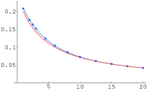
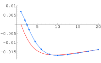
Figure 2: Numerical results for the exponents $\zeta_{1}$ and $\zeta_{2}$ for different values of $N$ (top). Numerical plots of $\zeta_{1}(N)$ (bottom/left) and $\zeta_{2}(N)$ (bottom/right), in blue with the numerical values from the table as dots. The red curves (no dots) represent the asymptotic expansion.

Although for SR disorder no analytical expression can be found for $\zeta_{1}$ and $\zeta_{2}$, their large-$N$ behavior can be obtained from an asymptotic analysis of (16). Let us extend the analysis of Balents and Fisher (BF) balents_fisher . Define $h=1/N\hat{h}$, $y=r^{2}/2$ and $\hat{h}(r)=Q(y)$. For $y\gg 1$ the FRG equation can be linearized:

$$(\epsilon-2\zeta)Q^{\prime}+2\zeta yQ^{\prime\prime}-(A+3B)Q^{\prime\prime}-2ByQ^{\prime\prime\prime}=0$$ (17)

with $A=(1-\frac{1}{N})Q^{\prime}_{0}+\frac{N-1}{4N^{2}}\hat{h}^{\prime\prime\prime}(0)^{2}$ and $B=\frac{1}{N}Q^{\prime}_{0}+\frac{N+3}{8N^{2}}\hat{h}^{\prime\prime\prime}(0)^{2}$, $\hat{h}^{\prime\prime}(0)=Q^{\prime}(0)=Q^{\prime}_{0}$. BF noted that there is an overlapping region $1\gg y\gg N$ where the solution can also be found perturbatively by expansion in $1/N$, yielding for $Q$ a pure exponential. It is indeed an exact solution of (17), with a unique value for $\zeta_{1}$, the BF result $\zeta_{1}\approx\zeta_{1}^{0}$ with $\zeta_{1}^{0}=1/(4+N)$ (i.e. the result from the replica variational method mezard_parisi ). The corrections (which arise from the neglected non-linear terms) are shown to be exponentially small; a more accurate estimate being $\zeta_{1}\approx\zeta_{1}^{1}$ with $\zeta_{1}^{1}=\zeta_{1}^{0}+(N+2)^{2}/(N+4)^{2}2^{-(N+2)/2}/(4e)$. To next order we find similarly the approximation to $\zeta_{2}$ footnoteeps :

$$\zeta_{2}^{0}=-\frac{(N^{2}-1)(2+N)}{2(4+N)^{3}(3+N)}\ ,$$ (18)

Figure 3: Results for the roughness $\zeta$ at 1- and 2-loop order, as a function of the number of components $N$. We both show a direct extrapolation and the Pade (1,1): $\zeta_{\mathrm{Pade}}=\frac{\epsilon\zeta_{1}}{1-\epsilon\zeta_{2}/\zeta_{1}}$.

where we have not attempted to estimate further corrections, presumably again exponentially small at large $N$. We note that $\zeta_{2}^{0}$ arises from the anomalous terms only. These estimates are listed and plotted on Fig. 2 together with the numerical solution of (16). The quality of the large-$N$ analysis is quite remarkable.

We now discuss the extrapolation of our result to the directed polymer (DP) case $d=1$, $\epsilon=3$, plotted in Fig. 3. We see that the 2-loop corrections are rather big at large $N$, so extrapolation down to $\epsilon=3$ is difficult. However both 1- and 2-loop results as well as the Pade-(1,1) reproduce well the two known points on the curve: $\zeta=2/3$ for $N=1$ KPZ and $\zeta=0$ for $N=\infty$ largeN . This branch in Fig. 3 corresponds to zero temperature and a continuum model. On the other hand we find that for all curves in figure 3 the roughness $\zeta$ becomes smaller than the thermal $\zeta_{\mathrm{th}}=\frac{1}{2}$ at $N=N_{\mathrm{uc}}\approx 2.5$. This naturally suggests the scenario that at non-zero temperature $\zeta=1/2$ for $N\geq N_{\mathrm{uc}}$, i.e. $N_{\mathrm{uc}}$ is the upper critical dimension vortices . The same argument gives an upper critical dimension $N_{\mathrm{uc}}$ for the KPZ-equation of non-linear surface growth KPZ ; Laessig . On the other hand, simulations on discretized models of both the directed polymer (at $T=0$) and the KPZ equation KPZsimu ; MarinariPagnaniParisi2000 suggest that $\zeta>1/2$ in all dimensions, but should be taken with caution footKPZ . Since the FRG is a systematic expansion in $\epsilon=4-d$, such a scenario seems reconcilable with our above results only through non-perturbative corrections in $\epsilon$, possibly non-analytic at $\epsilon=2$.

To conclude we have obtained for the $N$-component model a FRG description at 2-loop order. Various studies, including at large $N$, are under way to obtain a better understanding of the structure of the theory. For the KPZ growth and the directed polymer we have improved the determination of the possible upper critical dimension. Further numerics, in particular for the directed polymer at $T=0$ would be helpful.

References

- (1) G. Grüner, Rev. Mod. Phys. 60, 1129 (1988). A. Rosso and T. Giamarchi, Phys. Rev. B 70, 224204 (2004).
- (2) G. Blatter et al., Rev. Mod. Phys. 66, 1125 (1994).
- (3) T.Giamarchi and P. Le Doussal, Phys. Rev. B 52, 1242 (1995). T. Nattermann and S. Scheidl, Adv. Phys. 49, 607 (2000).
- (4) S. Moulinet, C. Guthmann, E. Rolley, Eur. Phys. J. A8 437 (2002)
- (5) S. Lemerle et al. Phys. Rev. Lett. 80, 849 (1998).
- (6) See reviews in Spin glasses and random fields Ed. A. P. Young, World Scientific, Singapore, 1998.
- (7) K. Efetov, A. Larkin, Sov. Phys. JETP 45, 1236 (1977).
- (8) M. Kardar, G. Parisi, and Y.-C. Zhang, Phys. Rev. Lett. 56, 889 (1986). M. Kardar, Nucl. Phys. B 290, 582 (1987).
- (9) B.M. Forrest and L.-H. Tang, Phys. Rev. Lett. 64, 1405 (1990); J.M. Kim, M.A. Moore, and A.J. Bray, Phys. Rev. A 44, 2345 (1991);
- (10) E. Marinari, A. Pagnani, and G. Parisi, J. Phys. A 33, 8181 (2000).
- (11) M. Lässig and H. Kinzelbach, Phys. Rev. Lett. 78, 903 (1997), M. Lässig, Phys. Rev. Lett. 80, 2366-2369 (1998).
- (12) D.S. Fisher, Phys. Rev. Lett. 56, 1964 (1986).
- (13) L. Balents and D.S. Fisher, Phys. Rev. B 48, 5959 (1993).
- (14) T. Nattermann et al., J. Phys. (Paris) 2, 1483 (1992). O. Narayan and D. S. Fisher, Phys. Rev. B 46, 11520 (1992).
- (15) H. Bucheli et al., Phys. Rev. B 57, 7642 (1998).
- (16) P. Chauve, P. Le Doussal and K.J. Wiese, Phys. Rev. Lett. 86, 1785 (2000).
- (17) S. Scheidl, unpublished; S. Scheidl and Y. Dincer, cond-mat/0006048; Y. Dincer, Diplomarbeit, Köln 1999.
- (18) P. Le Doussal, K.J. Wiese and P. Chauve, Phys. Rev. B 66, 174201 (2002).
- (19) P. Le Doussal, K.J. Wiese and P. Chauve, Phys. Rev. E 69, 026112 (2004).
- (20) P. Le Doussal and K.J. Wiese, Phys. Rev. Lett. 89, 125702 (2002); Phys. Rev. B 68, 174202 (2003); Nuclear Physics B 701, 409 (2004).
- (21) L. Balents and P. Le Doussal, Europhys. Lett. 65, 685 (2004).
- (22) L. Balents and P. Le Doussal, cond-mat/0408048, to appear in Adv. in Physics.
- (23) P. Chauve et al., Phys. Rev. B 62, 6241 (2000).
- (24) P. Chauve and P. Le Doussal, Phys. Rev. E. 64, 051102 (2001).
- (25) M. Mézard and G. Parisi, J. Phys. I 1, 809 (1991).
- (26) K.J. Wiese and P. Le Doussal, in preparation.
- (27) For the model one must have and the absence of super-cusp reads .
- (28) An alternative scenario is that a non-linear cusp with dimension-dependent exponent develops, e.g. . It may require deviations from the simplest scenario of a uniform density of shocks of codimension one.
- (29) We use the 1-loop relation .
- (30) Note that the UV-cutoff of the RSOS model in MarinariPagnaniParisi2000 is in the middle of the scaling plots for high dimensions.