Effects of Self-field and Low Magnetic Fields on the Normal-Superconducting Phase Transition

Abstract

Researchers have studied the normal-superconducting phase transition in the high-$T_{c}$ cuprates in a magnetic field (the vortex-glass or Bose-glass transition) and in zero field. Often, transport measurements in “zero field” are taken in the Earth’s ambient field or in the remnant field of a magnet. We show that fields as small as the Earth’s field will alter the shape of the current vs. voltage curves and will result in inaccurate values for the critical temperature $T_{c}$ and the critical exponents $\nu$ and $z$, and can even destroy the phase transition. This indicates that without proper screening of the magnetic field it is impossible to determine the true zero-field critical parameters, making correct scaling and other data analysis impossible. We also show, theoretically and experimentally, that the self-field generated by the current flowing in the sample has no effect on the current vs. voltage isotherms.

There continues to be a great deal of interest in the normal-superconducting phase transition of the cuprate superconductors, due in part to the accessibility of the critical regimechris and also to the well-understood theories regarding the transition.ffh This interest has generated a large body of work regarding the phase transition in a magnetic field (the vortex-glass or Bose-glass transition).see-doug This phase transition is generally accepted to exist,tinkham though reserachers have found very different results for the critical exponents $\nu$ and $z$.see-doug The existence of a vortex-glass transition has been debated by some,against and our own recent work has suggested a more precise criterion for determining the critical parameters if such a phase transition does indeed exist.doug

Much of the knowledge from the in-field transition carries over to the zero-field transition. This phase transition is less often studied, although paradoxically, the existence of this phase transition is not in doubt and the model that governs the phase transition is better understood. Like many other second-order phase transitions, the normal-superconducting phase transition in zero field is expected to obey the three-dimensional (3D) XY model with correlation length critical exponent $\nu=0.67$. If the dynamics are diffusive, then the expected dynamic critical exponent is $z=2$.ffh ; hh However, there are widely varying experimental results in zero field. Researchers have studied the bulk properties of $\mathrm{YBa_{2}Cu_{3}O_{7-\delta}}$ (YBCO), properties such as the specific heat,crit thermal expansivity,thermex and transport in single crystals,yeh and have reported critical exponents similar to those of the 3D-XY model, while others have found both 3D-XY and mean field exponents ($\nu=\frac{1}{2}$) in crystals.MFandgauss Transport measurements in thin-film YBCO have yielded exponents similar to those predicted by 3D-XY theory when extrapolating from high fields to zero field,moloni while measurements in low fields yield exponents larger than those expected from 3D-XY theory ($\nu\approx 1.1$, $z\approx 8.3$).lowfields Measurements on $\mathrm{Bi_{2}Sr_{2}CaCu_{2}O_{8+\delta}}$ (BSCCO), a similar hole-doped cuprate superconductor, yield similarly conflicting results in zero field: in crystals, there has been reported a 2D to 3D crossoverrapp1 as well as a critical regime with multiple exponents;rapp2 this multiple critical regime has also been observed in thin films,peligrad while other measurements on films claim to see 3D diffusive dynamicsosborn and still others see a 2D Kosterlitz-Thouless transition in this material.sefrioui

Our work on this complex topic has called into question the method most researchers previously used to analyze the data and has suggested a criterion for determining the existence of a phase transition and also for determining the critical parameters.doug We have also pointed out the often-overlooked effects of current noise on non-linear current vs. voltage ($I-V$) curves,noise and argued that the wide range of critical exponents in films of thickness $d\gtrsim 2000$ Å  is due to finite size effects limiting the size of the fluctuations.me

In this report we continue our re-examination of this topic and discuss the effects of low magnetic fields on transport measurements of the 3D zero-field normal-superconducting phase transition. The signature of the 3D phase transition is a change from linear behavior ($V\sim I$) at low currents above $T_{c}$ to nonlinear behavior ($V\sim I^{a}$) below $T_{c}$. We show that, in a manner similar to current noise,noise magnetic fields as low as the Earth’s magnetic field can change the shape of the $I-V$ curves and even create ohmic behavior in non-linear isotherms. Our results on 3D samples (similar to results found in 2D samples)garland indicate that if the magnetic field is not screened, the data analysis will yield an artificially low value for $T_{c}$ and inaccurate values for $\nu$ and $z$. Given how forgiving the scaling analysis can be,doug this is a possible source of the widely varying results in zero magnetic field. We will also discuss another possible source of magnetic fields: the self-field generated by the current in the sample.

We have used $I-V$ curves of YBCO to examine the normal-superconducting phase transition in zero field. Our films are deposited via pulsed laser deposition onto $\mathrm{SrTiO_{3}}$ (100) substrates. X-ray diffraction verified that our films are of predominately c-axis orientation, and ac susceptibility measurements showed transition widths $\leq 0.25$ K. $R(T)$ measurements show $T_{c}\approx 91.5$ K and transition widths of about 0.7 K. AFM and SEM images show featureless surfaces with a roughness of $\approx 12$ nm. These films are of similar or better quality than most YBCO films reported in the literature.

We photolithographically patterned our films into 4-probe bridges of width 8 $\mathrm{\mu}$m and length 40 $\mathrm{\mu}$m and etched them with a dilute solution of phosphoric acid without noticeable degradation of $R(T)$. Our cryostat can routinely achieve temperature stability of better than 1 mK at 90 K. To reduce noise, our cryostat is placed inside a screened room and all connections to the apparatus are made using shielded tri-axial cables.

Figure 1: $I-V$ curves for a 2200 Å thick film with bridge dimensions 8 $\mu$m $\times\ 40\ \mu$m. We can see that even a field as small as the Earth’s magnetic field (50 $\mu$T) is enough to alter the shape of the $I-V$ curves, and twice the Earth’s field (100 $\mu$T) can significantly change the shape of the isotherms. A field of 1 mT can create ohmic tails in isotherms which are non-linear in zero field. The $I-V$ curves are independent of the direction of the magnetic field. The isotherms are separated by 0.2 K.

It is well-known that magnetic fields will alter the shape of the $I-V$ curves. For this reason, we surround our cryostat with $\mu$-metal shields to reduce the ambient field to $2\times 10^{-7}$ T, as measured with a calibrated Hall sensor. It is generally assumed, however, that magnetic fields on the order of the Earth’s field (50-100 $\mu$T) or even remnant fields inside the bore of a superconducting magnet ($\sim$ 10 mT) are too small to affect the zero-field transition, making our $\mu$-metal shields superfluous. We have used the shields to test this assumption, however, by attaching a copper-wire solenoid to the outside of the vacuum can and applying small magnetic fields to the sample. We applied fields parallel to the c-axis and measured the resulting $I-V$ curves.nohysteresis These curves are shown in Fig. 1.

In the isotherm at 90.2 K in Fig. 1, we can see that a field as small as 50 $\mu$T will alter the shape of the $I-V$ curve. At 90.0 K and below, we can see that a field of 1 mT (10 G) – ten times smaller than the remnant field inside most magnets – can create an ohmic tail in non-linear isotherms. We also see in Fig. 1 that magnetic fields have the largest effect at low currents, whereas at current densities greater than $10^{8}$ A/m², the magnetic field has no effect on the isotherms. Because the clearest evidence for the transition is expected to occur at low currents, this fact is especially detrimental: it indicates that small magnetic fields have the largest effect precisely where we look for the signature of the phase transition. Thus, if the magnetic field is not screened out, then the false ohmic tails due to small magnetic fields at low currents will artificially decrease $T_{c}$ and consequently increase the value for the exponent $z$ derived from the data analysis, which will in turn lead to an inaccurate value for the exponent $\nu$.

The literature often reports measurements in “zero field,” however, it is unclear whether these measurements were taken inside of a shielded cryostat or in ambient field or inside the remnant field of a magnet. Because of the extreme sensitivity of the $I-V$ curves to even very small magnetic fields, this may be an explanation for the wide range of critical exponents reported. Moreover, our results indicate that true zero-field results may differ even from the results taken in ambient or “low” fields. Finally, our results indicate that only with proper shielding of external sources of magnetic field can you be assured of measuring the true zero-field properties of the sample.

This result leads directly to the next question: Even if we have shielded our cryostat of external sources, how can we be assured of eliminating all the internal sources of magnetic field? Twisted pair and distancing our $I-V$ bridge from the current-carrying wires will reduce the magnetic field from the current sources, however, there is one source of magnetic field that we cannot eliminate: the self-field created by the current in the sample. Is the magnetic field at the edge of the bridge large enough to create an effect similar to that created by external fields?

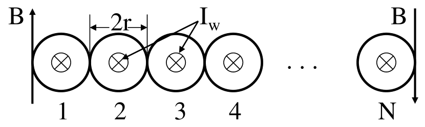
Figure 2: Approximation of the $I-V$ bridge as a collection of $N=w/d$ wires of radius $r=d/2$. The strongest fields occur at the edges of the wires, denoted by B in the figure.

To answer this question, we can approximate any bridge with thickness $d$ and width $w$ as $N=w/d$ parallel wires, each of radius $r=d/2$ carrying current $I_{w}$, as sketched in Fig. 2. We can then use Ampere’s law to determine the magnetic field $B$ at the edges of the bridge, as $B=\frac{\mu_{o}I_{w}}{2\pi r}+\frac{\mu_{o}I_{w}}{2\pi(3r)}+\frac{\mu_{o}I_{w}}{2\pi(5r)}+\cdots$. If the current density in each wire is given by $J$, and the total current in the bridge is $I$ (such that $I_{w}=I/N$), then:

$$B=\frac{1}{4}\mu_{o}dJ\sum_{i=1}^{N}\frac{1}{2i-1},$$ (1)

where $J=\frac{4}{\pi dw}I$. Typical films range in thickness from 100 nm to 300 nm and can be anywhere from 5 $\mu$m to 3 mm wide. Our own bridges have $w=8$ $\mu$m and $d=2000$ Å, giving $N=40$.

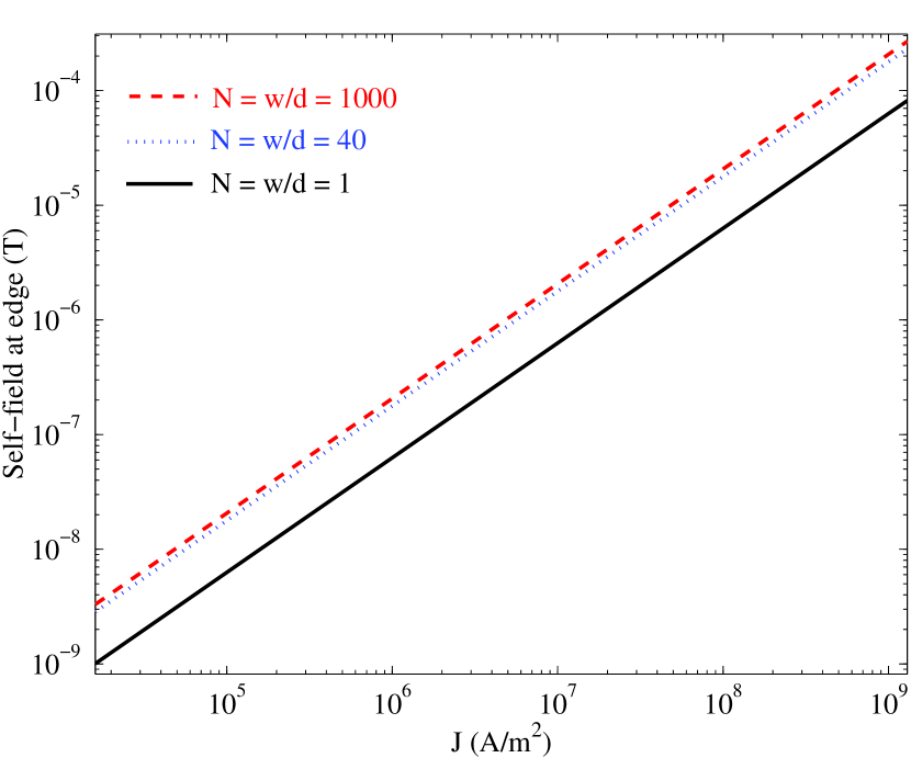
Figure 3: The self-field generated at the edges of an $I-V$ bridge for three values of $N=w/d$. We see that for $J\approx 10^{8}$ A/m², $B\approx 10$ $\mu$T, which may be large enough to affect the sample. Our bridges have $N=40$.

We plot $B$ for three values of $N$ in Fig. 3. We can see that at the higher current densities ($J\approx 10^{8}$ A/m²), the self-field will create fields on the order of 10 $\mu$T. At the low current densities where the phase transition is expected to be most apparent ($J\approx 10^{6}-10^{7}$ A/m²), the fields generated by the bridge are less than 1 $\mu$T. From this approximation, we expect the self-field to have no effect on the $I-V$ curves of the sample. At low currents, the self-field is too small to have any effect, and Fig. 1 indicates even a field of 10 or 100 $\mu$T has no effect at higher currents.

To verify that the self-field has no effect on the $I-V$ curves we conducted an experiment based on an earlier experiment in Josephson junction arraysjjarray designed to reduce the self-field at the edges of the sample. We patterned a film of YBCO to 8 $\mu$m $\times\ 40\ \mu$m and then covered the bridge with photoresist and patterned a gold bridge directly above the YBCO bridge. The two bridges were separated by 1.1 $\mu$m of photoresist and were not connected electrically. Using this geometry, we can flow a given current in the YBCO bridge and the same current in the opposite direction in the gold bridge. Although the field from the gold bridge will not exactly cancel the field from the YBCO bridge due to their separation, we can flow a higher current in the gold bridge to compensate for this. If the self-field generated by the YBCO bridge does create ohmic tails at low currents, we expect the ohmic tails to disappear when we flow a current in the opposite direction in the gold bridge. We can also flow current in the gold bridge in the same direction as the current in the YBCO bridge. In this case, if the self-field is generating ohmic tails, we expect the low-current ohmic tails to increase in resistance.

Figure 4: $I-V$ curves for a 2050 Å thick YBCO film with bridge dimensions 8 $\mu$m $\times\ 40\ \mu$m. A bridge of gold of thickness 2000 Å was patterned directly on top of YBCO film. The gold and YBCO bridges were separated by a layer of photoresist 1.1 $\mu$m thick. The solid lines are isotherms with no current flowing in the gold bridge. The $I-V$ points measured with different currents in the gold bridge are represented as triangles: $\nabla$ if the current in the gold bridge flows in the same direction as the current in the YBCO bridge, $\triangle$ if it flows against the current in the YBCO bridge. The colors represent the amount of current in the gold bridge: black, $10^{-7}$ A; red, $10^{-6}$ A; green, $10^{-4}$ A; blue, $10^{-2}$ A. The current in the gold bridge has no effect on the $I-V$ curves until we flow 10 mA of current in the gold bridge, which heats the YBCO bridge underneath. The isotherms are separated by 0.1 K. The error in the points is the size of the points.

We plot the results of this experiment in Fig. 4. In this figure, the solid lines indicate $I-V$ curves with no current in the gold bridge. $I-V$ points taken with current flowing in the gold bridge are shown as triangles. The $\nabla$ symbol represents the gold-bridge current flowing in the same direction as the YBCO bridge (expected to increase the ohmic tails); the $\triangle$ symbol represents the gold-bridge current flowing in the opposite direction as the YBCO bridge (expected to decrease the ohmic tails). The colors indicate various levels of current in the gold bridge. For clarity, results for only two temperatures and several currents in the YBCO bridge are presented, other temperatures and currents yield similar results.

In Fig. 4, there is no difference between the $\nabla$ symbols and the $\triangle$ symbols, indicating the $I-V$ points are independent of the direction of current flow in the gold bridge. There is also no deviation in the $I-V$ curves at any point or at any current in the gold bridge up to 10^-4 A. In fact, we only see an effect when we apply 10 mA to the gold bridge, which then raises the $I-V$ points across the entire $I-V$ curve. This is a result of the large power generated in the gold bridge at 10 mA, the heat from which is transferred to the YBCO bridge, raising its temperature. These results confirm the results of Figs. 1 and 3, namely, that the self-field generated by the bridge is too small to appreciably change the measured $I-V$ curve.

In conclusion, we have shown that magnetic fields as small as the Earth’s magnetic field (50 $\mu$T) can change the shape of the zero-field $I-V$ curves and create ohmic tails at low currents. Because a change from linear to non-linear behavior at low currents is the expected signature of the normal-superconducting phase transition, even small magnetic fields can lead to an underestimate of $T_{c}$, an overestimate of $z$, and inaccurate values for $\nu$. This indicates that to measure the zero-field phase transition correctly, the external magnetic field must be carefully screened out. We have also examined the self-field generated by the bridge itself, and have shown, theoretically and experimentally, that the self-field generated by the bridge is too small to appreciably affect the zero-field isotherms.

The authors thank D. Tobias, S. Li, H. Xu, M. Lilly, A. J. Berkley, Y. Dagan, H. Balci, M. M. Qazilbash, F. C. Wellstood, R. L. Greene, and especially J. Higgins for their help and discussions on this work. We acknowledge the support of the National Science Foundation through Grant No. DMR-0302596.

References

- (1) C. J. Lobb, Phys. Rev. B 36, 3930 (1987).
- (2) D. S. Fisher, M. P. A. Fisher, and D. A. Huse, Phys. Rev. B 43, 130 (1991); D. A. Huse, D. S. Fisher, and M. P. A. Fisher, Nature 358, 553 (1992).
- (3) See Ref. doug, for an abbreviated list of the papers examining the normal-superconducting phase transition in a magnetic field.
- (4) M. Tinkham, Introduction to Superconductivity, 2nd ed. p. 356-361 (Dover, New York, 2004).
- (5) S. N. Coppersmith, M. Inui, and P. B. Littlewood, Phys. Rev. Lett. 64, 2585 (1990); B. Brown, Phys. Rev. B 61, 3267 (2000); Z. L. Xiao, J. Häring, Ch. Heinzel, and P. Ziemann, Sol. State Comm. 95, 153 (1995); H. S. Bokil and A. P. Young, Phys. Rev. Lett. 74, 3021 (1995); C. Wengel and A. P. Young, Phys. Rev. B 54, R6869 (1996); H. Kawamura, J. Phys. Soc. Jpn. 69, 29 (2000);
- (6) D. R. Strachan, M. C. Sullivan, P. Fournier, S. P. Pai, T. Venkatesan and C. J. Lobb, Phys. Rev. Lett. 87, 067007 (2001); D. R. Strachan, M. C. Sullivan, and C. J. Lobb, Proc. SPIE 4811, 65-77 (2002).
- (7) P. C. Hohenberg and B. I. Halperin, Rev. Mod. Phys. 49, 435 (1977).
- (8) N. Overend, M. A. Howson, and I. D. Lawrie, Phys. Rev. Lett. 72, 3238 (1994); G. Mozurkewich, M. B. Salamon, and S. E. Inderhees, Phys. Rev. B 46, 11914 (1992); S. Kamal, D. A. Bonn, N. Goldenfeld, P. J. Hirschfeld, R. Liang, and W. N. Hardy, Phys. Rev. Lett. 73, 1845 (1994).
- (9) V. Pasler, P. Schweiss, C. Meingast, B. Obst, H. Wühl, A. I. Rykov, and S. Tajima, Phys. Rev. Lett. 81, 1094 (1998).
- (10) N.-C. Yeh, W. Jiang, D. S. Reed, U. Kriplani and F. Holtzberg, Phys. Rev. B 47, 6146 (1992); N.-C. Yeh, D. S. Reed, W. Jiang, U. Kriplani, F. Holtzberg, A. Gupta, B. D. Hunt, R. P. Vasquez, M. C. Foote, and L. Bajuk, Phys. Rev. B 45, 5654 (1992).
- (11) P. Pureur, R. Menegotto Costa, P. Rodrigues Jr., J. Schaf, and J. V. Kunzler, Phy. Rev. B 47 11420 (1993); A. Pomar, A. Diaz, M. V. Ramallo, C. Torron, J. A. Veira, and Felix Vidal, Physica C 218, 257 (1993).
- (12) K. Moloni, M. Friesen, S. Li, V. Souw, P. Metcalf, L. Hou, and M. McElfresh, Phys. Rev. Lett. 78, 3173 (1997).
- (13) C. Dekker, R.H. Koch, B. Oh and A. Gupta, Physica C 185-189, 1799 (1991); J. M. Roberts, Brandon Brown, B. A. Hermann, and J. Tate, Phys. Rev. B 49, 6890 (1994); T. Nojima, T. Ishida, and Y. Kuwasawa, Czech. Jour. Phys. 46 Suppl. S3, 1713 (1996);
- (14) S. H. Han, Yu. Eltsev, and O. Rapp, Phys. Rev. B, 57, 7510 (1998).
- (15) S. H. Han, Yu. Eltsev, and O. Rapp, Phys. Rev. B, 61, 11776 (2000).
- (16) D.-N. Peligrad, M. Mehring, and A. Dulcic, Phys. Rev. B 69, 144516 (2004).
- (17) K. D. Osborn, D. J. Van Harlingen, V. Aji, N. Goldenfeld, S. Oh, and J. N. Eckstein, Phys. Rev. B 68 144516 (2003).
- (18) Z. Sefrioui, D. Arias, C. Leon, J. Santamaria, E. M. Gonzalez, J. L. Vicent, and P. Prieto, Phys. Rev. B 70, 064502 (2004).
- (19) M. C. Sullivan, T. Frederiksen, J. M. Repaci, D. R. Strachan, R. A. Ott, and C. J. Lobb, Phys Rev B 70, 140503(R) (2004).
- (20) M. C. Sullivan, D. R. Strachan, T. Frederiksen, R. A. Ott, M. Lilly, and C. J. Lobb, Phys. Rev. B 69, 214524 (2004).
- (21) J. C. Garland and H. J. Lee, Phys. Rev. B 36, 3638 (1987).
- (22) We have also reversed the magnetic field, and found that the direction of the magnetic field (parallel or anti-parallel to the c-axis) has no effect on the curve, i.e., there is no hysteresis in the sample, as expected.
- (23) H. C. Lee, R. S. Newrock, D. B. Mast, S. E. Hebboul, J. C. Garland, and C. J. Lobb, Phys. Rev. B 44, R921 (1991).