Dynamics of channel incision in a granular bed driven by subsurface water flow

Abstract

We propose a dynamical model for the erosive growth of a channel in a granular medium driven by subsurface water flow. The model is inferred from experimental data acquired with a laser-aided imaging technique. The evolution equation for transverse sections of a channel has the form of a non-locally driven Burgers equation. With fixed coefficients this equation admits an asymptotic similarity solution. Ratios of the granular transport coefficients can therefore be extracted from the shape of channels that have evolved in steady driving conditions.

One of the salient features of fluvial erosion is the formation and growth of channels Dietrich and Dunne (1993). The channels act to focus the flow of water, either over land Horton (1945), or, ubiquitously but less commonly appreciated, beneath the surface Dunne (1990). Here we address the dynamics of erosion driven by subsurface flow. Whereas flow through the subsurface is well characterized by Darcy’s law Sheidegger (1960); Bear (1972), channel formation and growth resulting from seepage flows out of the surface is relatively poorly understood Schörghofer et al. (2004). This erosive process is important not only because of its relevance to enigmatic features of natural landscapes Howard and McLane (1988); Laity and Malin (1985); Schumm et al. (1995); Orange et al. (1994); Higgins (1982); Schörghofer et al. (2004); Wentworth (1928); Kochel and Piper (1986); Malin and Edgett (2000), but also because it raises fundamental questions concerning the continuum mechanics of wet sand Daerr et al. (2003); Huang et al. (2005); Fournier et al. (2005); Tegzes et al. (2003); Schulz et al. (2003); Jain et al. (2004, 2001); Zhou et al. (2005).

In this Letter we construct a theoretical model of the erosive dynamics of an isolated channel. The model is inferred from data acquired with a laser-aided imaging technique. In our experiment we grow a single channel under controlled driving conditions and acquire maps of the evolving granular surface that are highly resolved in space and time. We find that transverse sections of a channel evolve according to a non-locally driven Burgers equation. Under steady driving conditions the evolution equation admits a similarity solution, thereby relating erosive transport coefficients to channel geometry.

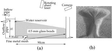
Figure 1: (a) Schematic of our experimental setup. (b) Example of an isolated channel observed after 90 minutes of subsurface water flow driven growth. A small initial channel is incised on the surface to fix the location and number of channels. Similar shapes are observed if channels form spontaneously.

Figure 1 shows a schematic of the experiment, aspects of which are described in more detail elsewhere Schörghofer et al. (2004); Lobkovsky et al. (2004). Water enters beneath a pile of identical glass beads through a fine mesh and exits at the foot of the pile through the same kind of mesh. The water flux is controlled by the height $H$ of the water column in a reservoir behind the pile. The slope of the initial sandpile as well as the water column height are the control variables of the experiment. Since the water table is convex upward in this geometry Lobkovsky et al. (2004), we are able to finely control the amount of water on the surface of the granular pile. Refs. Schörghofer et al. (2004) and Lobkovsky et al. (2004) describe the phenomenology of the pattern formation in this setup and quantify the transitions between various modes of granular flow: surface flow (responsible for the formation of the channel network), slumping (bulk frictional instability) and fluidization.

Here we focus on the late-stage evolution of an isolated channel that grows from a short initial channel of triangular crossection. A scanning laser imaging technique allows us to measure the evolving height of the sandpile with sub-grain resolution in space and one-minute resolution in time. A laser sheet scans the surface while a digital camera acquires images from an oblique angle. The height of the surface is then extracted from an image of the intersection of the laser sheet with the granular surface.

The water level $H$ is set below the threshold for erosion outside the channel but above the threshold for erosion in the channel. An example of a channel grown from an initial channel with a triangular crossection is shown in Fig. 1(b). We find that the late stage morphology of the channel is insensitive to the exact initial condition as long as the initial incision is sufficiently deep.

Figure 2: Residual erosion rate at $t=39$ min plotted against (a) the slope, (b) the curvature, and (c) the fractional channel depth. Each symbol represents an average over several hundred data points. To obtain the residual erosion rate we subtract from the measured $\dot{h}$ the terms on the right hand side of Eq. (1) which depend on the variables other than the one against which the erosion rate is being plotted. Lines are drawn using the parameters extracted by a least squares fit of the unbinned data to equation (1). Error bars represent two standard deviations of the mean.

We seek an effective description of the channel’s evolution in terms of the surface height $h(x,y,t)$ measured from the uneroded surface. In other words, we seek an expression for the erosion rate $\dot{h}\equiv\partial h/\partial t$ in terms of $h$, its spatial derivatives, and possibly spatial integrals. (Here $y$ is the downslope axis and $x$ is the axis transverse to the channel). This approach is reasonable because the relaxation of the water flux toward steady state is fast compared to the erosion rate. Thus the water flux is a functional of the slowly changing shape of the channel.

The erosion rate is a function of the local water and granular fluxes. In steady state these fluxes are functionals of the global shape of the granular pile. We seek to reduce the global dependence to a single scalar by arguing that, because the channel evolves in a roughly self-similar manner, the water fluxes (bulk as well as surficial) are functions of the local topography and a time-varying scale factor. We choose the channel depth $h_{0}(y)$ as this scale factor ($h_{0}$ corresponds to height of the deepest point of the crossection). We have thus reduced the problem to finding the dependence of the erosion rate on the local topography and the overall global scale factor.

We make one more simplification: we consider solely the evolution of transverse sections of the channel, and therefore express the erosion rate $\dot{h}\equiv\partial h/\partial t$ through $h$ and its derivatives with respect to the transverse coordinate $x$ only. Variation of the water flow in the downslope $y$-direction is accounted for via $y$-dependent coefficients. This approximation is reasonable everywhere except the top portion of the channel’s head where the downslope gradient varies rapidly. Grains and microscopic avalanches enter and leave a given channel transect. Projected onto this transect, the transport of height $h$ is no longer volume conserving.

Thus, the erosion rate $\dot{h}$ is assumed to be a function of the fractional depth $h/h_{0}$, the transverse slope $h_{x}=\partial h/\partial x$, and the curvature $h_{xx}=\partial^{2}h/\partial x^{2}$. Our approach is to measure these quantities for data in a window of duration $\Delta t$ in time and length $\Delta y$ in the downslope coordinate and to fit the resulting data cloud via a least squares method to the form

$$\dot{h}=\nu h_{xx}-\delta|h_{x}|-\lambda h_{x}^{2}-\mu\,\Theta(h/h_{0}-f),$$ (1)

where $\Theta(x)$ is the Heaviside step function. The empirical constants $\mu$, $\nu$, $\lambda$, $\delta$, and $f$ are functions of time $t$ and downslope coordinate $y$. They encode the microscopic properties of the grain dynamics as well as the strength of the driving water flow. The diffusion constant $\nu$ reflects the rate of smoothing of local perturbations. The last term on the right hand side represents driving due to the seeping water. We assume that driving is constant below a fraction $f$ of the total channel depth and null above this fractional depth. The second and third terms on the right hand side of (1) are advective. We hypothesize that perturbations are advected only up the slope, similar to Ref. Boutreux et al. (1998). Therefore, the non-analytic term $\delta|h_{x}|$ corresponds to advection of perturbations with velocity $\delta$ independent of slope, whereas $\lambda h_{x}^{2}$ corresponds to advection with velocity $\lambda h_{x}$, which grows linearly with slope.

Figure 2 illustrates the fit of the data to the model. As shown in Fig. 2(a), the slope dependent terms make the largest contribution into the erosion rate. Data points with slopes smaller than 0.7, comprising over 95% of all data, have been used in the fit. A discrepancy between the model and the data occurs for larger slopes where the erosion rate saturates. A measurable contribution to the erosion rate due to diffusion is shown in Fig. 2(b). The extracted positive granular diffusivity $\nu$ is statistically significant. The driving, depth-dependent term, shown in Fig. 2(c), is approximated by a step function although the data show a more gradual transition. We expect the width of the transition region to remain constant as the channel grows. Thus the step function approximation should improve with time.

We extract the time-dependent coefficients in Eq. (1) near a transect fixed in the lab frame. Fig. 3 shows the extracted parameters for a transect initially above the pre-dug channel. As the channel head migrates past this transect, the driving $\mu$ peaks and declines. The values of advection speeds $\delta$ and $\lambda$ also decrease since they are related to the driving. The diffusion coefficient $\nu=0.039\pm 0.033$ mm²/min and the fractional driving $f=0.52\pm 0.14$ fluctuate around their respective means which are roughly time-independent.

Figure 3: Example of the evolution of the coefficients $\mu$, $\lambda$ and $\delta$ (measured in mm/min) extracted using Eq. (1) from the data using taken near a fixed transect illustrated in Fig. 4. The head of the channel arrives to this transect approximately one minute after the start of the experimental run.

In Fig. 4(a) and (b) we indicate in a contour plot of the channel the location of the transect for which the parameters in Fig. 3 are computed. Fig. 4(c) compares the measured shapes of this transect with the shapes evolved via Eq. (1) with the time-dependent coefficients. Agreement indicates that the right hand side of Eq. (1) captures the essential features of the erosion rate in the channel geometry. The rate of advance of the channel sidewalls and the receding rate of channel bottom are determined by different combinations of the parameters. The match of the evolved shapes to the data shows that both rates are in accord with the experiment.

In our experiment the coefficients, intimately related to the geometry of the water flow, change markedly during the evolution of the channel as illustrated in Fig. 3. It is conceivable, however, that in other geometries the transport coefficients are approximately constant over a long time. It is therefore appropriate to examine the long-time behavior of Eq. (1) with constant coefficients. The rest of the paper is devoted to the asymptotic calculation.

The main result is that the non-local driving term in Eq. (1) allows for an asymptotically self-similar growing channel shape. To see that let us define a scale factor $\ell(t)$ and the shape $Y(\xi,t)$, which is a function of the scaled coordinate $\xi=x/\ell(t)$ via a transformation $h(x,t)=\ell(t)\,Y(\xi,t)$. Further progress results from a formal expansion

$$Y(\xi,t) = Y_{0}(\xi)+\frac{1}{t}\,Y_{1}(\xi)+\ldots,$$ (2a)

$$\ell(t) = t+\ell_{1}\ln t+\ldots.$$ (2b)

The zeroth order shape $Y_{0}(\xi)$ is independent of time. Thus, if the expansion (2) converges, the shape converges (albeit slowly as $1/t$) to a similarity solution $Y_{0}$. A substitution of the expansion (2) into (1) yields, at the lowest order,

$$Y_{0}-\xi Y_{0}^{\prime}=-\beta Y_{0}^{\prime}-\alpha(Y_{0}^{\prime})^{2}-\Theta\left(\frac{Y_{0}}{Y_{0}(0)}-f\right),$$ (3)

where primes denote differentiation with respect to $\xi$. We scaled lengths by $a=\nu/\mu$ and time by $\tau=\nu/\mu^{2}$ and defined $\beta=\delta/\mu$ and $\alpha=\lambda/\mu$. Note that the diffusive term does not enter at the lowest order. The physical reason for this is that, as we show below, diffusion is important on a fixed length scale. As the channel grows larger than this diffusive length, the $h_{xx}$ term in (1) becomes negligible compared to the advection and the driving terms.

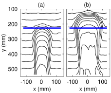
Figure 4: Contour plots of the laser height data at (a) $t=15$ min and (b) 115 min after the start of the water flow. The thick line shows the location of the modeled transect. The contour interval is 5 mm. (c) Same transect at $t=$ 15, 45, and 115 min compared to the prediction of Equation (1). The smoothed shape of the transect at $t=15$ min was used as the initial condition. Actual time dependent parameters presented in Fig. 3 were used.

The solution to (3) must be symmetric with respect to $\xi\rightarrow-\xi$ and smooth everywhere except at the fractional driving point $\xi_{0}$ where $Y_{0}(\xi_{0})=fY_{0}(0)$. It turns out that there exists a one-parameter family of similarity solutions which satisfy these criteria. These solutions are constructed as follows. In the driven region any piece of the parabola

$$Y_{0}(\xi)=\frac{1}{4\alpha}\left(\xi^{2}-2\beta\xi+\beta^{2}-4\alpha\right),$$ (4)

and a tangent line to this parabola at a point $\xi_{1}$,

$$Y_{0}(\xi)=\frac{1}{4\alpha}\left(2\xi(\xi_{1}-\beta)+\beta^{2}-\xi_{1}^{2}-4\alpha\right),$$ (5)

are solutions to (3). In the undriven region, the trivial solution $h=0$ as well as tangents to the parabola

$$Y_{0}(\xi)=\frac{1}{4\alpha}\left(\xi^{2}-2\beta\xi\right)$$ (6)

are solutions. A smooth solution symmetric around $\xi=0$ is therefore constructed from four pieces:

$$Y_{0}=\begin{cases}-1,&0<\xi<\xi_{b},\\ -1+\frac{(\xi-\xi_{b})^{2}}{4\alpha},&\xi_{b}<\xi<\xi_{1},\\ -1+\frac{(\xi_{1}-\xi_{b})^{2}}{4\alpha}+\frac{(\xi_{1}-\xi_{b})(\xi-\xi_{1})}{2\alpha},&\xi_{1}<\xi<\xi_{0}\\ -f+s_{0}(\xi-\xi_{0}),&\xi_{0}<\xi<\xi_{e}.\end{cases}$$ (7)

The first piece is the flat bottom of the channel tangent to the parabola (4) at its apex $\xi_{b}=\beta$, $Y_{0}=-1$. The second piece is part of the parabola itself. The third piece is another tangent to parabola (4) at a point $\xi_{1}$ such that $\beta\leq\xi_{1}\leq\beta+\sqrt{4\alpha(1-f)}$. The fourth piece is the tangent of slope $s_{0}$ to the undriven parabola (6). Note that $Y_{0}$ is not smooth at $\xi_{0}$ (driving) and $\xi_{e}$ (channel edge).

It turns out that the diffusive term, though not present at zeroth order, acts to select a unique member from the one-parameter family of similarity solutions. The selection mechanism, verified by numerical methods, is unclear to us at this time. The selected similarity solution is one in which the second tangent to the parabola (4) is missing, i.e., $\xi_{1}$ assumes its upper limit. The slope of the sidewall of the channel in the undriven region is then simply

$$s_{0}=\frac{1}{\sqrt{\alpha}}(1+\sqrt{1-f}).$$ (8)

The expressions for $\xi_{0}$ and $\xi_{e}$ are simple as well:

$$\xi_{0}=\beta+\sqrt{4\alpha(1-f)},\quad\xi_{e}=\xi_{0}+f/s_{0}$$ (9)

We remark that the asymptotic shape consisting of a flat bottom, curved parabolic flanks in the driven region followed by straight sidewalls can be used successfully to fit channel crossections which evolve in non-steady conditions. However, the ratios of parameters extracted by such an asymptotic fit can deviate greatly from the parameters extracted by the fit of the equation (1) to the data cloud, because the shape of the channel at the time of the fit retains a memory of its prior dynamical state.

Besides selecting the unique self-similar shape, the diffusive term also acts to smooth slope discontinuities at $\xi_{0}$ and $\xi_{e}$. An exact expression for this smoothing can be obtained at the channel’s edge $\xi_{e}$. In the vicinity of this point, the slope $s=h_{x}$ is a hyperbolic tangent

$$s(x,t)=\frac{s_{0}}{2}\left(1-\tanh{\frac{s_{0}\alpha}{2}(x-vt)}\right),$$ (10)

moving with velocity $v=s_{0}\alpha+\beta$ and smooth on a scale

$$R=\frac{2\nu}{\sqrt{\lambda\mu}(1+\sqrt{1-f})}.$$ (11)

As we mentioned above, diffusion acts on a fixed scale $R$. The smoothing of the kink at $\xi=\xi_{0}$ is probably related to the selection of the unique similarity solution.

Guided by an experiment, we have developed a phenomenological model of granular dynamics in a transect of a channel eroded by subsurface fluid flow. Precise, time resolved measurements of the height of the eroding sandpile allow us to test the validity of the model. The erosion rate is a function of the local topography and an overall scale factor. We expect this approximation to be good as long as the channel’s shape remains roughly self-similar. There are five parameters in the model which in our experiment vary with time. These parameters encode the geometry of the water flow as well as the features of the microscopic granular flow. In a different water flow geometry these parameters can remain roughly constant. In this case the height evolution equation (1) admits a self-similar solution and the three dimensionless parameters $\alpha$, $\beta$ and $f$ dictate the self-similar shape. Conversely, if a shape is known to have resulted from evolution with roughly constant parameters, then $\alpha$, $\beta$ and $f$ can be extracted from the static shape. Given an independent measure of the erosion rate $\mu$ at the bottom of the channel, as well as the measurement of the smoothing length scale $R$ at the channel’s edge, all five parameters can be recovered. Such a procedure should be useful for the analysis of natural channels formed by subsurface fluid flow.

This work is supported by DOE grants DE–FG02–02ER15367 at Clark University and DE–FG02–99ER15004 at MIT.

References

- Dietrich and Dunne (1993) W. E. Dietrich and T. Dunne, in Channel Network Hydrology, edited by K. Beven and M. J. Kirby (John Wiley and Sons Ltd, New York, 1993), pp. 175–219.
- Horton (1945) R. E. Horton, Geological Society of America Bulletin 56, 275 (1945).
- Dunne (1990) T. Dunne, in Special Paper 252 (Geological Society of America, Boulder, CO, 1990), pp. 1–28.
- Sheidegger (1960) A. E. Sheidegger, The Physics of Flow Through Porous Media (Macmillan Company, New York, 1960).
- Bear (1972) J. Bear, Dynamics of Fluids in Porous Media (Dover Publications, New York, 1972).
- Schörghofer et al. (2004) N. Schörghofer, B. Jensen, A. Kudrolli, and D. H. Rothman, J. Fluid Mech. 503, 357 (2004).
- Howard and McLane (1988) A. D. Howard and C. F. McLane, Water Resources Research 24, 1659 (1988).
- Laity and Malin (1985) J. E. Laity and M. C. Malin, Geol. Soc. Am. Bull. 96, 203 (1985).
- Schumm et al. (1995) S. A. Schumm, K. F. Boyd, C. G. Wolff, and W. J. Spitz, Geomorphology 12, 281 (1995).
- Orange et al. (1994) D. L. Orange, R. S. Anderson, and N. A. Breen, GSA Today 4, 1 (1994).
- Higgins (1982) C. G. Higgins, Geology 10, 147 (1982).
- Wentworth (1928) C. K. Wentworth, J. Geol. 36, 385 (1928).
- Kochel and Piper (1986) R. C. Kochel and J. F. Piper, J. Geophys. Res. 91, E175 (1986).
- Malin and Edgett (2000) M. C. Malin and K. Edgett, Science 288, 2330 (2000).
- Huang et al. (2005) N. Huang, G. Ovarlez, F. Bertrand, S. Rodts, P. Coussot, and D. Bonn, Phys. Rev. Lett. 94, 028301 (2005).
- Fournier et al. (2005) Z. Fournier, D. Geromichalos, S. Herminghaus, M. M. Kohonen, F. Mugele, M. Scheel, M. Schulz, B. Schulz, C. Schier, R. Seemann, et al., J. Phys.–Cond. Mat. 17, S477 (2005).
- Tegzes et al. (2003) P. Tegzes, T. Vicsek, and P. Schiffer, Phys. Rev. E 67, 051303 (2003).
- Schulz et al. (2003) M. Schulz, B. M. Schulz, and S. Herminghaus, Phys. Rev. E 67, 052301 (2003).
- Jain et al. (2004) N. Jain, J. M. Ottino, and R. M. Lueptow, J. FLuid Mech. 508, 23 (2004).
- Jain et al. (2001) N. Jain, D. V. Khakhar, R. M. Lueptow, and J. M. Ottino, Phys. Rev. E 86, 3771 (2001).
- Zhou et al. (2005) J. Zhou, A. Bertozzi, B. Dupuy, and A. E. Hosoi, Phys. Rev. Lett. 94, 117803 (2005).
- Daerr et al. (2003) A. Daerr, P. Lee, J. Lanuza, and E. Clement, Phys. Rev. E 67, 065201 (pages 4) (2003).
- Lobkovsky et al. (2004) A. E. Lobkovsky, W. Jensen, A. Kudrolli, and D. H. Rothman, J. Geophys. Res.–Earth Surface 109, 1 (2004).
- Boutreux et al. (1998) T. Boutreux, E. Raphael, and P. G. de Gennes, Phys Rev. E 58, 4692 (1998).