Critical behavior and Griffiths effects in the disordered contact process

Abstract

We study the nonequilibrium phase transition in the one-dimensional contact process with quenched spatial disorder by means of large-scale Monte-Carlo simulations for times up to $10^{9}$ and system sizes up to $10^{7}$ sites. In agreement with recent predictions of an infinite-randomness fixed point, our simulations demonstrate activated (exponential) dynamical scaling at the critical point. The critical behavior turns out to be universal, even for weak disorder. However, the approach to this asymptotic behavior is extremely slow, with crossover times of the order of $10^{4}$ or larger. In the Griffiths region between the clean and the dirty critical points, we find power-law dynamical behavior with continuously varying exponents. We discuss the generality of our findings and relate them to a broader theory of rare region effects at phase transitions with quenched disorder.

I Introduction

The nonequilibrium behavior of many-particle systems has attracted considerable attention in recent years. Of particular interest are continuous phase transitions between different nonequilibrium states. These transitions are characterized by large scale fluctuations and collective behavior over large distances and times very similar to the behavior at equilibrium critical points. Examples of such nonequilibrium transitions can be found in population dynamics and epidemics, chemical reactions, growing surfaces, and in granular flow and traffic jams (for recent reviews see, e.g., Refs. SchmittmannZia95 ; Marro_book ; Dickman ; chopard_book ; Hinrichsen00 ; Odor ; tauber_rev )

A prominent class of nonequilibrium phase transitions separates active fluctuating states from inactive, absorbing states where fluctuations cease entirely. Recently, much effort has been devoted to classifying possible universality classes of these absorbing state phase transitions Hinrichsen00 ; Odor . The generic universality class is directed percolation (DP) dp . According to a conjecture by Janssen and Grassberger conjecture , all absorbing state transitions with a scalar order parameter, short-range interactions, and no extra symmetries or conservation laws belong to this class. Examples include the transitions in the contact process contact , catalytic reactions ziff , interface growth tang , or turbulence turb . In the presence of conservation laws or additional symmetries, other universality classes can occur, e.g., the parity conserving class Takayasu92 ; Zhong95 ; Tauber96 or the $Z_{2}$-symmetric directed percolation (DP2) class KimPark94 ; Menyhard94 ; Hinrichsen97 .

In realistic systems, one can expect impurities and defects, i.e., quenched spatial disorder, to play an important role. Indeed, it has been suggested that disorder may be one of the reasons for the surprising rarity of experimental realizations of the ubiquitous directed percolation universality class hinrichsen_exp . The only verification so far seems to be found in the spatio-temporal intermittency in ferrofluidic spikes spikes .

The investigation of disorder effects on the DP transition has a long history, but a coherent picture has been slow to emerge. According to the Harris criterion harris ; Noest86 , a clean critical point is stable against weak disorder if the spatial correlation length critical exponent $\nu_{\perp}$ fulfills the inequality

$$d\nu_{\perp}>2,$$ (1)

where $d$ is the spatial dimensionality. The DP universality class violates the Harris criterion in all dimensions $d<4$, because the exponent values are $\nu_{\perp}\approx 1.097$ (1D), 0.73 (2D), and 0.58 (3D) Hinrichsen00 . A field-theoretic renormalization group study janssen97 confirmed the instability of the DP critical fixed point. Moreover, no new critical fixed point was found. Instead the renormalization group displays runaway flow towards large disorder, indicating unconventional behavior. Early Monte-Carlo simulations Noest86 showed significant changes in the critical exponents while later studies moreira of the two-dimensional contact process with dilution found logarithmically slow dynamics in violation of power-law scaling. In addition, rare region effects similar to Griffiths singularities Griffiths were found to lead to slow dynamics in a whole parameter region in the vicinity of the phase transition moreira ; Noest88 ; bramson ; webman ; cafiero .

Recently, an important step towards understanding spatial disorder effects on the DP transition has been made by Hooyberghs et al. hooyberghs . These authors used the Hamiltonian formalism alcaraz to map the one-dimensional disordered contact process onto a random quantum spin chain. Applying a version of the Ma-Dasgupta-Hu strong-disorder renormalization group SDRG , they showed that the transition is controlled by an infinite-randomness critical point, at least for sufficiently strong disorder. This type of fixed point leads to activated (exponential) rather than power-law dynamical scaling. For weaker disorder, Hooyberghs et al. hooyberghs used computer simulations and predicted non-universal continuously varying exponents, with either power-law or exponential dynamical correlations.

In this paper, we present the results of large-scale Monte-Carlo simulations of the one-dimensional contact process with quenched spatial disorder. Using large systems of up to $10^{7}$ sites and very long times (up to $10^{9}$) we show that the critical behavior at the nonequilibrium phase transition is indeed described by an infinite-randomness fixed point with activated scaling. Moreover, we provide evidence that this behavior is universal, i.e., it occurs even in the weak-disorder case. However, the approach to this universal asymptotic behavior is extremely slow, with crossover times of the order of $10^{4}$ or larger which may explain why nonuniversal (effective) exponents have been seen in previous work. We also study the Griffiths region between the clean and the dirty critical points. Here, we find power-law dynamical behavior with continuously varying exponents, in agreement with theoretical predictions.

This paper is organized as follows. In section II, we introduce the model. We then contrast power-law scaling as found at conventional critical points with activated scaling arising from infinite-randomness critical points. We also summarize the predictions for the Griffiths region. In section III, we present our simulation method and the numerical results together with a comparison to theory. We conclude in section IV by discussing the generality of our findings and their relation to a broader theory of rare region effects at phase transitions with quenched disorder.

II Theory

II.1 Contact process with quenched spatial disorder

We start from the clean contact process contact , a prototypical system in the DP universality class. It can be interpreted, e.g., as a model for the spreading of a disease. The contact process is defined on a $d$-dimensional hypercubic lattice. Each lattice site $\mathbf{r}$ can be active (occupied by a particle) or inactive (empty). In the course of the time evolution, active sites can infect their neighbors, or they can spontaneously become inactive. Specifically, the dynamics is given by a continuous-time Markov process during which particles are created at empty sites at a rate $\lambda n/(2d)$ where $n$ is the number of active nearest neighbor sites. Particles are annihilated at rate $\mu$ (which is often set to unity without loss of generality). The ratio of the two rates controls the behavior of the system.

For small birth rate $\lambda$, annihilation dominates, and the absorbing state without any particles is the only steady state (inactive phase). For large birth rate $\lambda$, there is a steady state with finite particle density (active phase). The two phases are separated by a nonequilibrium phase transition in the DP universality class at $\lambda=\lambda_{c}^{0}$. The central quantity in the contact process is the average density of active sites at time $t$

$$\rho(t)=\frac{1}{L^{d}}\sum_{\mathbf{r}}\langle n_{\mathbf{r}}(t)\rangle$$ (2)

where $n_{\mathbf{r}}(t)$ is the particle number at site $\mathbf{r}$ and time $t$, $L$ is the linear system size, and $\langle\ldots\rangle$ denotes the average over all realizations of the Markov process. The longtime limit of this density (i.e., the steady state density)

$$\rho_{\rm stat}=\lim_{t\to\infty}\rho(t)$$ (3)

is the order parameter of the nonequilibrium phase transition.

Quenched spatial disorder can be introduced by making the birth rate $\lambda$ a random function of the lattice site $\mathbf{r}$. We assume the disorder to be spatially uncorrelated; and we use a binary probability distribution

$$P[\lambda({\mathbf{r}})]=(1-p)\,\delta[\lambda({\mathbf{r}})-\lambda]+p\,\delta[\lambda({\mathbf{r}})-c\lambda]$$ (4)

where $p$ and $c$ are constants between 0 and 1. This distribution allows us to independently vary spatial density $p$ of the impurities and their relative strength $c$. The impurities locally reduce the birth rate, therefore, the nonequilibrium transition will occur at a value $\lambda_{c}$ that is larger than the clean critical birth rate $\lambda_{c}^{0}$.

II.2 Conventional power-law scaling

In this subsection we summarize the phenomenological scaling theory of an absorbing state phase transition that is controlled by a conventional fixed point with power-law scaling (see, e.g., Ref. Hinrichsen00 ). The clean contact process falls into this class.

In the active phase and close to critical point $\lambda_{c}$, the order parameter $\rho_{\rm stat}$ varies according to the power law

$$\rho_{\rm stat}\sim(\lambda-\lambda_{c})^{\beta}\sim\Delta^{\beta}$$ (5)

where $\Delta=(\lambda-\lambda_{c})/\lambda_{c}$ is the dimensionless distance from the critical point, and $\beta$ is the critical exponent of the particle density. In addition to the average density, we also need to characterize the length and time scales of the density fluctuations. Close to the transition, the correlation length $\xi_{\perp}$ diverges as

$$\xi_{\perp}\sim|\Delta|^{-\nu_{\perp}}~{}.$$ (6)

The correlation time $\xi_{\parallel}$ behaves like a power of the correlation length,

$$\xi_{\parallel}\sim\xi_{\perp}^{z},$$ (7)

i.e., the dynamical scaling is of power-law form. Consequently the scaling form of the density as a function of $\Delta$, the time $t$ and the linear system size $L$ reads

$$\rho(\Delta,t,L)=b^{\beta/\nu_{\perp}}\rho(\Delta b^{-1/\nu_{\perp}},tb^{z},Lb)~{}.$$ (8)

Here, $b$ is an arbitrary dimensionless scaling factor.

Two important quantities arise from initial conditions consisting of a single active site in an otherwise empty lattice. The survival probability $P_{s}$ describes the probability that an active cluster survives when starting from such a single-site seed. For directed percolation, the survival probability scales exactly like the density betaprime ,

$$P_{s}(\Delta,t,L)=b^{\beta/\nu_{\perp}}P_{s}(\Delta b^{-1/\nu_{\perp}},tb^{z},Lb)~{}.$$ (9)

Thus, for directed percolation, the three critical exponents $\beta$, $\nu_{\perp}$ and $z$ completely characterize the critical point.

The pair connectedness function $C(\mathbf{r^{\prime}},t^{\prime},\mathbf{r},t)=\langle n_{\mathbf{r^{\prime}}}(t^{\prime})\,n_{\mathbf{r}}(t)\rangle$ describes the probability that site $\mathbf{r}^{\prime}$ is active at time $t^{\prime}$ when starting from an initial condition with a single active site at $\mathbf{r}$ and time $t$. For a clean system, the pair connectedness is translationally invariant in space and time. Thus, it only depends on two arguments $C(\mathbf{r},t^{\prime},\mathbf{r},t)=C(\mathbf{r^{\prime}}-\mathbf{r},t-t^{\prime})$. Because $C$ involves a product of two densities, its scale dimension is $2\beta/\nu_{\perp}$, and the full scaling form reads hyperscaling

$$C(\Delta,\mathbf{r},t,L)=b^{2\beta/\nu_{\perp}}C(\Delta b^{-1/\nu_{\perp}},\mathbf{r}b,tb^{z},Lb)~{}.$$ (10)

The total number of particles $N$ when starting from a single seed site can be obtained by integrating the pair connectedness $C$ over all space. This leads to the scaling form

$$N(\Delta,t,L)=b^{2\beta/\nu_{\perp}-d}N(\Delta b^{-1/\nu_{\perp}},tb^{z},Lb)~{}.$$ (11)

At the critical point, $\Delta=0$, and in the thermodynamic limit, $L\to\infty$, the above scaling relations lead to the following predictions for the time dependencies of observables: The density and the survival probability asymptotically decay like

$$\rho(t)\sim t^{-\delta},\qquad P_{s}(t)\sim t^{-\delta}$$ (12)

with $\delta=\beta/(\nu_{\perp}z)$. In contrast, the number of particles in a cluster starting from a single seed site increases like

$$N(t)\sim t^{\Theta}$$ (13)

where $\Theta=d/z-2\beta/(\nu_{\perp}z)$ is the so-called critical initial slip exponent.

Highly precise estimates of the critical exponents for clean one-dimensional directed percolation have been obtained by series expansions Jensen99 : $\beta=0.276486$, $\nu_{\perp}=1.096854$, $z=1.580745$, $\delta=0.159464$, and $\Theta=0.313686$.

II.3 Activated scaling

In this subsection we summarize the scaling theory for an infinite-randomness fixed point with activated scaling, as has been predicted to occur in absorbing state transitions with quenched disorder hooyberghs . It is similar to the scaling theory for the quantum phase transition in the random transverse field Ising model dsf9295 .

At an infinite-randomness fixed point, the dynamics is extremely slow. The power-law scaling (7) gets replaced by activated dynamical scaling

$$\ln(\xi_{\parallel})\sim\xi_{\perp}^{\psi},$$ (14)

characterized by a new exponent $\psi$. This exponential relation between time and length scales implies that the dynamical exponent $z$ is formally infinite. In contrast, the static scaling behavior remains of power law type.

Moreover, at an infinite-randomness fixed point the probability distributions of observables become extremely broad, so that averages are dominated by rare events such as rare spatial regions with large infection rate. In such a situation, averages and typical values of a quantity do not necessarily agree. Nonetheless, the scaling form of the average density at an infinite-randomness critical point is obtained by simply replacing the power-law scaling combination $tb^{z}$ by the activated combination $\ln(t)b^{\psi}$ in the argument of the scaling function:

$$\rho(\Delta,\ln(t),L)=b^{\beta/\nu_{\perp}}\rho(\Delta b^{-1/\nu_{\perp}},\ln(t)b^{\psi},Lb)~{}.$$ (15)

Analogously, the scaling forms of the average survival probability and the average number of sites in a cluster starting from a single site are

$$P_{s}(\Delta,\ln(t),L) = b^{\beta/\nu_{\perp}}P_{s}(\Delta b^{-1/\nu_{\perp}},\ln(t)b^{\psi},Lb)$$ (16)

$$N(\Delta,\ln(t),L) = b^{2\beta/\nu_{\perp}-d}N(\Delta b^{-1/\nu_{\perp}},\ln(t)b^{\psi},Lb)~{}~{}.$$ (17)

These activated scaling forms lead to logarithmic time dependencies at the critical point (in the thermodynamic limit). The average density and the survival probability asymptotically decay like

$$\rho(t)\sim[\ln(t)]^{-\bar{\delta}},\qquad P_{s}(t)\sim[\ln(t)]^{-\bar{\delta}}$$ (18)

with $\bar{\delta}=\beta/(\nu_{\perp}\psi)$ while the average number of particles in a cluster starting from a single seed site increases like

$$N(t)\sim[\ln(t)]^{\bar{\Theta}}$$ (19)

with $\bar{\Theta}=d/\psi-2\beta/(\nu_{\perp}\psi)$. These are the relations we are going to test in this paper.

Within the strong disorder renormalization group approach of Ref. hooyberghs , the critical exponents of the disordered one-dimensional contact process can be calculated exactly. Their numerical values are $\beta=0.38197$, $\nu_{\perp}=2$, $\psi=0.5$, $\bar{\delta}=0.38197$, and $\bar{\Theta}=1.2360$.

II.4 Griffiths region

The inactive phase of our disordered contact process with the impurity distribution (4) can be divided into two regions. For birth rates below the clean critical point, $\lambda<\lambda_{c}^{0}$, the behavior is conventional. The system approaches the absorbing state exponentially fast in time. The decay time increases with $\lambda$ and diverges as $|\lambda-\lambda_{c}^{0}|^{-z\nu_{\perp}}$ where $z$ and $\nu_{\perp}$ are the exponents of the clean critical point Bray88 ; Dickison05 .

The more interesting region is the so-called Griffiths region Noest86 ; Griffiths which occurs for birth rates between the clean and the dirty critical points, $\lambda_{c}^{0}<\lambda<\lambda_{c}$. The system is globally still in the inactive phase, i.e., the system eventually decays into the absorbing state. However, in the thermodynamic limit, one can find arbitrarily large spatial regions devoid of impurities. For $\lambda_{c}^{0}<\lambda<\lambda_{c}$, these so-called rare regions are locally in the active phase. Because they are of finite size, they cannot support a non-zero steady state density but their decay is very slow because it requires a rare, exceptionally large density fluctuation.

The contribution of the rare regions to the time evolution of the density can be estimated as follows Noest86 ; Noest88 . The probability $w$ for finding a rare region of linear size $L_{r}$ devoid of impurities is (up to pre-exponential factors) given by

$$w(L_{r})\sim\exp(-\tilde{p}L_{r}^{d})$$ (20)

where $\tilde{p}$ is a nonuniversal constant which for our binary disorder distribution is given by $\tilde{p}=-\ln(1-p)$. The long-time decay of the density is dominated by these rare regions. To exponential accuracy, the rare region contribution to the density can be written as

$$\rho(t)\sim\int dL_{r}~{}L_{r}^{d}~{}w(L_{r})\exp\left[-t/\tau(L_{r})\right]$$ (21)

where $\tau(L_{r})$ is the decay time of a rare region of size $L_{r}$. Let us first discuss the behavior at the clean critical point, $\lambda_{c}^{0}$, i.e., at the boundary between the conventional inactive phase and the Griffiths region. At this point, the decay time of a single, impurity-free rare region of size $L_{r}$ scales as $\tau(L_{r})\sim L_{r}^{z}$ as follows from finite size scaling barber . Here $z$ is the clean critical exponent. Using the saddle point method to evaluate the integral (21), we find the leading long-time decay of the density to be given by a stretched exponential,

$$\ln\rho(t)\sim-\tilde{p}^{z/(d+z)}~{}t^{d/(d+z)}~{},$$ (22)

rather than a simple exponential decay as for $\lambda<\lambda_{c}^{0}$.

Inside the Griffiths region, i.e., for $\lambda_{c}^{0}<\lambda<\lambda_{c}$, the decay time of a single rare region depends exponentially on its volume,

$$\tau(L_{r})\sim\exp(aL_{r}^{d})$$ (23)

because a coordinated fluctuation of the entire rare region is required to take it to the absorbing state Noest86 ; Noest88 ; Schonmann85 . The nonuniversal prefactor $a$ vanishes at the clean critical point $\lambda_{c}^{0}$ and increases with $\lambda$. Close to $\lambda_{c}^{0}$, it behaves as $a\sim\xi_{\perp}^{-d}\sim(\lambda-\lambda_{c}^{0})^{d\nu_{\perp}}$ with $\nu_{\perp}$ the clean critical exponent. Repeating the saddle point analysis of the integral (21) for this case, we obtain a power-law decay of the density

$$\rho(t)\sim t^{-\tilde{p}/a}=t^{-d/z^{\prime}}$$ (24)

where $z^{\prime}=da/\tilde{p}$ is a customarily used nonuniversal dynamical exponent in the Griffiths region. Its behavior close to the dirty critical point $\lambda_{c}$ can be obtained within the strong disorder renormalization group method hooyberghs ; dsf9295 . When approaching the phase transition, $z^{\prime}$ diverges as $z^{\prime}\sim|\lambda-\lambda_{c}|^{-\psi\nu_{\perp}}$ where $\psi$ and $\nu_{\perp}$ are the exponents of the dirty critical point.

III Monte-Carlo simulations

III.1 Method and overview

We now turn to the main part of the paper, extensive Monte-Carlo simulations of the one-dimensional contact process with quenched spatial disorder. There is a number of different ways to actually implement the contact process on the computer (all equivalent with respect to the universal behavior). We follow the widely used algorithm described, e.g., by Dickman dickman99 . Runs start at time $t=0$ from some configuration of occupied and empty sites. Each event consists of randomly selecting an occupied site $\mathbf{r}$ from a list of all $N_{p}$ occupied sites, selecting a process: creation with probability $\lambda(\mathbf{r})/[1+\lambda(\mathbf{r})]$ or annihilation with probability $1/[1+\lambda(\mathbf{r})]$ and, for creation, selecting one of the neighboring sites of $\mathbf{r}$. The creation succeeds, if this neighbor is empty. The time increment associated with this event is $1/N_{p}$. Note that in this implementation of the disordered contact process both the creation rate and the annihilation rate vary from site to site in such a way that their sum is constant (and equal to one).

Using this algorithm, we have performed simulations for system sizes between $L=1000$ and $L=10^{7}$. We have studied impurity concentrations $p=0.2,0.3,0.4,0.5,0.6$ and 0.7 as well as relative impurity strengths of $c=0.2,0.4,0.6$ and 0.8. To explore the extremely slow dynamics associated with the predicted infinite-randomness critical point, we have simulated very long times up to $t=10^{9}$ which is, to the best of our knowledge, at least three orders of magnitude in $t$ longer than previous simulations of the disordered contact process. In all cases we have averaged over a large number of different disorder realizations, details will be mentioned below for each specific set of calculations.

Figure 1 gives an overview over the phase diagram resulting from our simulations.

Figure 1: Phase diagrams of the disordered contact process. Left: Birth rate $\lambda$ vs. impurity concentration $p$ for fixed impurity strength $c=0.2$. Right: $\lambda$ vs. $c$ for fixed $p=0.3$.

As expected, the critical birthrate $\lambda_{c}$ increases with increasing impurity concentration $p$. It also increases with decreasing birth rate on the impurities, i.e., a decreasing relative strength $c$. For $p=0$ or $c=1$, we reproduce the well-known clean critical birth rate $\lambda_{c}^{0}\approx 3.298$ Jensen93 . In the following subsections we discuss the behavior in the vicinity of the phase transition in more detail.

III.2 Time evolution starting from full lattice

In this subsection we discuss simulations which follow the time evolution of the average density starting from a full lattice. This means, at time $t=0$, all sites are active and $\rho(0)=1$.

Figure 2 gives an overview of the time evolution of the density for a system of $10^{6}$ sites with $p=0.3,c=0.2$, covering the $\lambda$ range from the conventional inactive phase, $\lambda<\lambda_{c}^{0}$ all the way to the active phase, $\lambda>\lambda_{c}$.

Figure 2: Overview of the time evolution of the density for a system of $10^{6}$ sites with $p=0.3$ and $c=0.2$. The clean critical point $\lambda_{c}^{0}\approx 3.298$ and the dirty critical point $\lambda_{c}\approx 5.24$ are specially marked.

The data are averages over 480 runs, each with a different disorder realization. For birth rates below and at the clean critical point $\lambda_{c}^{0}\approx 3.298$, the density decay is very fast, clearly faster then a power law. Above $\lambda_{c}^{0}$, the decay becomes slower and asymptotically seems to follow a power-law. For even larger birth rates the decay seems to be slower than a power law while the largest birth rates give rise to a nonzero steady state density, i.e., the system is in the active phase.

III.2.1 Griffiths region

Let us investigate the different parameter regions in more detail, beginning with the behavior at the clean critical point $\lambda_{c}^{0}$, i.e., at the boundary between the Griffiths region and the conventional absorbing phase. According to eq. (22), the density should asymptotically decay like a stretched exponential. To test this behavior, we plot the logarithm of the density as a function of $t^{d/(d+z)}$ where $d=1$ and $z\approx 1.581$ is the dynamical exponent of the clean one-dimensional contact process. Figure 3 shows the resulting graphs for system size $L=10^{7}$, $c=0.2$, and several impurity concentrations $p=0.2\ldots 0.7$.

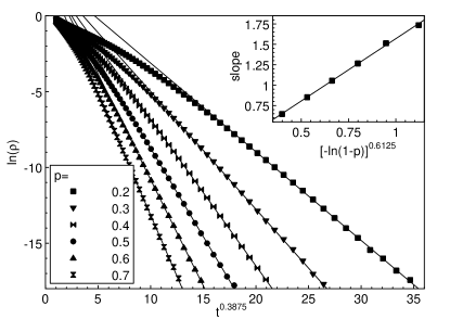
Figure 3: Time evolution of the density at the clean critical point $\lambda_{c}^{0}=3.298$ for systems of $10^{7}$ sites with $c=0.2$ and several $p$. The straight lines are fits to the stretched exponential $\ln\rho(t)\sim-Et^{d/(d+z)}$ predicted in eq. (22) with $d=1$ and the clean $z=1.580$. Inset: Decay constant $E$ vs. $\tilde{p}^{z/(d+z)}$.

The data are averages over 960 runs, each with a different disorder realization. The figure shows that the data follow a stretched exponential behavior $\ln\rho=-Et^{0.3875}$ over more than four orders of magnitude in $\rho$, in good agreement with eq. (22). The decay constant $E$, i.e., the slope of these curves, increases with increasing impurity concentration $p$. The inset of figure 3 shows the relation between $E$ and $\tilde{p}=-\ln(1-p)$. In good approximation, the values follow the power law $E\sim\tilde{p}^{z/(d+z)}=\tilde{p}^{0.6125}$ predicted in (22).

We now turn to the behavior inside the Griffiths region, $\lambda_{c}^{0}<\lambda<\lambda_{c}$. Figure 4 shows a double-logarithmic plot of the density time evolution for birth rates $\lambda=3.5\ldots 5.1$ and $p=0.3,c=0.2$. The system sizes are between $10^{6}$ and $10^{7}$ lattice sites, and we have averaged over 480 disorder realizations.

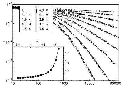
Figure 4: Log-log plot of the density time evolution in the Griffiths region for systems with $p=0.3,c=0.2$ and several birth rates $\lambda$. The system sizes are $10^{7}$ sites for $\lambda=3.5,3.7$ and $10^{6}$ sites for the other $\lambda$ values. The straight lines are fits to the power law $\rho(t)\sim t^{-1/z^{\prime}}$ predicted in eq. (24). Inset: Dynamical exponent $z^{\prime}$ vs. birth rate $\lambda$.

For all birth rates $\lambda$ shown, the long-time decay of the density asymptotically follows a power-law, as predicted in eq. (24), over several orders of magnitude in $\rho$ (except for the largest $\lambda$ where we could observe the power law only over a smaller range in $\rho$ because the decay is too slow).

The nonuniversal dynamical exponent $z^{\prime}$ can be obtained by fitting the long-time asymptotics of the curves in figure 4 to eq. (24). The inset of figure 4 shows $z^{\prime}$ as a function of the birth rate $\lambda$. As discussed in section II.4, $z^{\prime}$ increases with increasing $\lambda$ throughout the Griffiths region with an apparent divergence around $\lambda\approx 5.2$. Unfortunately, our data did not allow us to make quantitative comparisons with the predictions for the $\lambda$-dependence of $z^{\prime}$ because we could not reliably determine $z^{\prime}$ sufficiently close to either the clean critical point or the dirty critical point. Close to the clean critical point $\lambda_{c}^{0}$, the crossover to the asymptotic power law occurs at very low densities, thus the system size limits how close one can get to $\lambda_{c}^{0}$. Conversely, for larger $\lambda$ close to the dirty critical point $\lambda_{c}$, the crossover to the asymptotic power law occurs at very long times. Thus, the maximum simulation time limits how close to the dirty critical point one can still extract $z^{\prime}$.

III.2.2 Dirty critical point

After having discussed the Griffiths region, we now turn to the most interesting parameter region, the vicinity of the dirty critical point. In contrast to the clean critical birth rate $\lambda_{c}^{0}$ which is well known from the literature Jensen93 , the dirty critical birth rate $\lambda_{c}$ is not known a priori. In order to find $\lambda_{c}$ and at the same time test the predictions of the activated scaling picture of section II.3, we employ the logarithmic time dependence of the density, eq. (18). In figure 5 we plot $\rho^{-1/\bar{\delta}}$ with the predicted $\bar{\delta}=0.38197$ against $\ln(t)$ for a system of $10^{4}$ sites with $p=0.3$ and $c=0.2$.

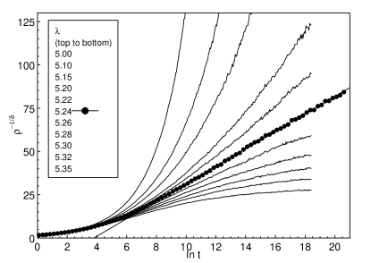
Figure 5: $\rho^{-1/\bar{\delta}}$ vs. $\ln(t)$ for a system of $10^{4}$ sites with $p=0.3$ and $c=0.2$. The filled circles mark the critical birth rate $\lambda_{c}=5.24$, and the straight line is a fit of the long-time behavior to eq. (18)

Because the dynamics at the dirty critical point is expected to be extremely slow, we have simulated up to $t=10^{8}$ ($10^{9}$ for the critical curve). As before, the data are averages over 480 runs, each with a different disorder realization.

In this type of plot, the logarithmic time dependence (18) is represented by a straight line. Subcritical data should curve upward from the critical straight line, while supercritical data should curve downward and eventually settle to a constant long-time limit. From the data in figure 5 we conclude that the dirty critical point indeed follows the activated scaling scenario associated with an infinite-randomness critical point. The critical birthrate is $\lambda_{c}=5.24\pm 0.01$. At this $\lambda$, the density follows eq. (18) over almost four orders of magnitude in $t$.

The statistical error of the plotted average densities can be estimated from the standard deviation of $\rho(t)$ between the 480 separate runs. For the critical curve, $\lambda=5.24$, in figure 5, the error of the average density remains below $0.002$ which corresponds to about a symbol size in the figure (at the long-time end of the plot). We have also checked for possible finite-size effects by repeating the calculation for a smaller system size of $L=10^{3}$. Within the statistical error the results for $L=10^{3}$ and $L=10^{4}$ are identical, from which we conclude that our data are not influenced by finite size effects.

III.2.3 Universality

We now turn to the questions of universality: Is the activated scaling scenario valid for all impurity concentrations $p$ and strengths $c$, and is the value of the critical exponent $\bar{\delta}$ the same for all cases? To answer these questions we have repeated the above critical point analysis for different sets of the disorder parameters $p$ and $c$. In this subsection, we first show that all these data are in agreement with the activated scaling scenario with an universal exponent $\bar{\delta}$. We then discuss whether they could interpreted in a conventional power-law scaling scenario as well.

In the first set of calculations we have kept the impurity concentration at $p=0.3$, but we have varied their relative strength from $c=0.2$ to 0.8. In all cases, the density decay at the respective dirty critical birth rate $\lambda_{c}$ follows the logarithmic law (18) with the predicted $\bar{\delta}=0.38197$ over several orders of magnitude in $t$. Figure 6 shows these critical curves for systems with $c=0.2,0.4,0.6$ and 0.8.

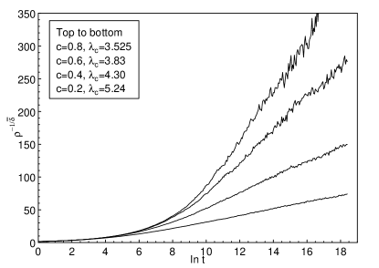
Figure 6: Time evolution of the density for systems of $10^{4}$ sites with $p=0.3$ and $c=0.2,0.4,0.6$ and 0.8 at their respective critical points plotted as $\rho^{-1/\bar{\delta}}$ vs. $\ln(t)$ as in figure 5.

The seemingly larger fluctuations for the curves with higher $c$ are caused by the way the data are plotted: The large negative exponent $-1/\bar{\delta}$ strongly stretches the low-density part of the ordinate.

We have obtained analogous results from the second set of runs where we kept $c=0.2$ constant but varied the impurity concentration from $p=0.2$ to 0.5. From these simulation results we conclude that the data are in agreement with the activated scaling scenario for all studied parameter values including the case of weak disorder. (Note that for $p=0.3,c=0.8$, the disorder-induced shift of the critical birthrate is small, ($\lambda_{c}-\lambda_{c}^{0})/\lambda_{c}^{0}\approx 0.07$.) Moreover, our results are compatible with a universal value of 0.38197 for the exponent $\bar{\delta}$.

However, we would like to emphasize that while our data do not show any indication of non-universality, we cannot exclude some variation of $\bar{\delta}$ with the disorder strength. This is caused by the fact that even though we observe the logarithmic time dependence (18) over almost four orders of magnitude in $t$, this corresponds only to about a factor of 2 to 3 in $\ln(t)$. This is a very small range for extracting the exponent of the power-law relation between $\rho$ and $\ln(t)$. More specifically, the asymptotic critical time dependence of the density for $p=0.3,c=0.2$ can be fitted by $\rho=(A*\ln(t)+B)^{-0.38197}$ with $A\approx 5.12$ and $B\approx-20.1$ (this is the straight line in figure 5). Comparison with eq. (18) shows that $B$ represents a correction to scaling. For a reliable extraction of the exponent one would want the $\ln(t)$ term to be at least one order of magnitude larger than $B$ at the very minimum. This corresponds to $\ln(t)\approx 40$ or $t\approx 10^{17}$ which is clearly unreachable in a Monte Carlo simulation for the foreseeable future.

We now turn to the question of whether the numerical data could also be interpreted in terms of conventional power-law scaling. To this end, we first replot the critical density decay curves as identified above CPIDENT in standard log-log form in Fig. 7.

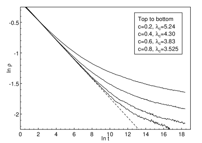
Figure 7: Replot of the data of figure 6 in log-log form. The dashed line shows a power-law decay with the clean critical exponent $\delta=0.159$.

This figure shows that the density decay at early times follows a power law with the clean decay exponent $\delta=0.159$. However, after some disorder dependent crossover time $t_{x}$ the curves show pronounced upward curvature. This curvature persists to the largest times and signifies an asymptotic decay that is slower than any power law. The crossover time $t_{x}$ which increases with decreasing disorder $c\to 1$ nicely agrees with the onset of the asymptotic logarithmic behavior in Fig. 6 for all disorder strengths. Thus, the time dependence of the density $\rho(t)$ directly crosses over from the clean critical (power law) behavior at short times to the activated (logarithmic) behavior (18) at large times. We find no indication of any power laws other than the clean one, not even at transient times. We thus conclude that our data, at least for times up to $t=10^{8}$ are not compatible with power-law scaling at the dirty critical point.

It would be highly desirable to discriminate between power-law and activated scaling by performing a full scaling analysis of the data using relations (8,9,11) or (15,16,17), respectively. Unfortunately, such an analysis is impossible because the extremely slow dynamics leads to the abovementioned strong corrections to scaling in the accessible range of times up to $t=10^{9}$.

III.3 Time evolution starting from a single particle

In addition to the simulations staring from a full lattice, we have also performed simulations of the time evolution starting from a single active site in an otherwise empty lattice. In these calculations, we have monitored the survival probability $P_{s}$ and the number of sites $N$ in the active cluster as functions of time. According to eqs. (18) and (19), these quantities are expected to behave as $P_{s}(t)\sim[\ln(t)]^{-1/\bar{\delta}}$ and $N(t)\sim[\ln(t)]^{\bar{\Theta}}$ at the dirty critical point.

Figure 8 shows plots of $P_{s}^{-\bar{\delta}}$ and $N^{1/\bar{\Theta}}$ vs. $\ln(t)$ for a system with $p=0.3$ and $c=0.2$.

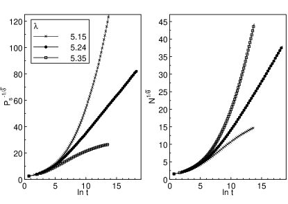
Figure 8: Survival probability $P_{s}$ and particle number $N$ in the active cluster for a simulation starting from single active site. The disorder parameters are $p=0.3$ and $c=0.2$.

The data are averages over 480 different disorder realizations. For each realization we have performed 200 runs starting from a single active site at a random position. The system size $L=10^{6}$ was several orders of magnitude larger than the largest active cluster, thus we have effectively simulated an infinite-size system. Figure 8 shows that $P_{s}$ and $N$ indeed follow the predicted logarithmic laws with $\bar{\delta}=0.38197$ and $\bar{\Theta}=1.236$ at the critical birthrate $\lambda_{c}=5.24$. Subcritical and supercritical data curve away from the critical straight lines as expected. Thus, the simulations starting from a single site also confirm the activated scaling scenario resulting from an infinite-randomness critical point.

III.4 Steady state

Lastly, we have studied the behavior of the steady state density in the active phase. Close to the critical point it is expected to vary as $\rho_{\rm stat}\sim(\lambda-\lambda_{c})^{\beta}$ with $\beta=0.38197$. These calculations require a particularly high numerical effort because the approach to the steady is logarithmically slow close to the critical point. Therefore, we have simulated up to $t=10^{9}$ for birthrates close to $\lambda_{c}$. Figure 9 shows the time evolution of the density in the active phase for a system with $p=0.3$ and $c=0.2$, averaged over 480 disorder realizations (one run per realization).

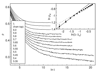
Figure 9: Time evolution of the density in the active phase for a system with $p=0.3$ and $c=0.2$. The system sizes are $10^{4}$ for $\lambda\geq 5.8$ and $10^{3}$ otherwise. Inset: Steady state density vs. distance from critical point. The solid line is a fit of the data for $\lambda-\lambda_{c}<0.3$ to the expected dirty power law $\rho_{\rm stat}\sim(\lambda-\lambda_{c})^{\beta}$ with $\beta=0.38197$. The dashed line is a fit of the data for $\lambda-\lambda_{c}>0.3$ to a power law with the clean $\beta=0.2765$.

The steady state densities can be obtained by averaging the constant part of each of the curves. The data clearly demonstrate the extremely slow approach to the steady state. For $\lambda\leq 5.4$ the steady state is not reached (within the statistical error) even after $t=10^{9}$. Therefore, our steady state density values for these $\lambda$ are only rough estimates.

The inset of figure 9 shows the resulting steady state densities plotted vs. the distance from the critical point. This graph nicely demonstrates the crossover from clean to dirty critical behavior. The data away from the critical point ($\lambda-\lambda_{c}>0.3$) can be well fitted by a power law with the clean value of the critical exponent $\beta=0.2765$. When approaching the critical point the curve becomes steeper, and for $\lambda-\lambda_{c}<0.3$ the data can be reasonably well fitted by a power law with the expected dirty critical exponent $\beta=0.38197$. The position of the crossover can be compared to an estimate from the time dependence at $\lambda_{c}$ in figure 5. The critical curve reaches its asymptotic logarithmic form at about $t_{x}\approx 10^{4}$ which corresponds to a crossover density of $\rho_{x}\approx 0.3$ in rough agreement with the crossover density in the inset of figure 9.

IV Conclusions

To summarize, we have presented the results of large-scale Monte-Carlo simulations of a one-dimensional contact process with quenched spatial disorder for large systems of up to $L=10^{7}$ sites and very long times up to $t=10^{9}$. These simulations show that the critical behavior at the nonequilibrium phase transition is controlled by an infinite-randomness fixed point with activated scaling and ultraslow dynamics, as predicted in Ref. hooyberghs . Moreover, the simulations provide evidence that this behavior is universal. The logarithmically slow time dependencies (18,19) are valid (with the same exponent values) for all parameter sets investigated including the weak-disorder case. However, the approach to this universal asymptotic behavior is extremely slow, with crossover times of the order of $10^{4}$ or larger. Since most of the earlier Monte-Carlo simulations did not exceed $t=10^{5}\ldots 10^{6}$ this may explain why nonuniversal (effective) exponents were seen in previous work. We have also presented results for the Griffiths region between the clean and the dirty critical points. Here, we have found power-law dynamical behavior with continuously varying exponents, in agreement with theoretical predictions Noest86 ; Noest88 .

We now discuss the relation of our results to a more general theory of rare region effects at phase transitions with quenched disorder. In Ref. VojtaSchmalian05 a general classification of phase transitions in quenched disordered systems with short-range interactions RKKY has been suggested, based on the effective dimensionality $d_{\rm eff}$ of the rare regions. Three cases can be distinguished.

(i) If $d_{\rm eff}$ is below the lower critical dimension $d_{c}^{-}$ of the problem, the rare region effects are exponentially small because the probability of a rare region decreases exponentially with its volume but the contribution of each region to observables increases only as a power law. In this case, the critical point is of conventional power-law type. Examples in this class include, e.g., the classical equilibrium Ising transition with point defects where $d_{\rm eff}=0$ and $d_{c}^{-}=1$.

(ii) In the second class, with $d_{\rm eff}=d_{c}^{-}$, the Griffiths effects are of power-law type because the exponentially rarity of the rare regions in $L_{r}$ is overcome by an exponential increase of each region’s contribution. In this class, the critical point is controlled by an infinite-randomness fixed point with activated scaling. Examples include the quantum phase transition in the random transverse field Ising model ($d_{\rm eff}=d_{c}^{-}=1)$ dsf9295 ; taufootnote as well as the transition discussed in this paper (where $d_{\rm eff}=d_{c}^{-}=0$).

(iii) Finally, for $d_{\rm eff}>d_{c}^{-}$, the rare regions can undergo the phase transition independently from the bulk system. This leads to a destruction of the sharp phase transition by smearing. This behavior occurs at the equilibrium Ising transition with plane defects where $d_{\rm eff}=2,d_{c}^{-}=1$ us_planar , the quantum phase transition in itinerant magnets us_rounding , and for the contact process with extended (line or plane) defects Dickison05 ; contact_pre .

Thus, the results of this paper do fit into the general rare-region based classification scheme of phase transitions with quenched disorder and short-range interactions VojtaSchmalian05 . These arguments also suggest that the behavior of the phase transition in a higher-dimensional disordered contact process should be controlled by an infinite-randomness fixed point as well.

We conclude by pointing out that the unconventional behavior found in this paper may explain the striking absence of directed percolation scaling hinrichsen_exp in at least some of the experiments. However, the extremely slow dynamics will prove to be a challenge for the verification of the activated scaling scenario not just in simulations but also in experiments.

References

- (1) B. Schmittmann and R.K.P. Zia, in Phase transitions and critical phenomena, edited by C. Domb and J.L. Lebowitz, Vol. 17, (Academic, New York 1995)
- (2) J. Marro and R. Dickman, Nonequilibrium Phase Transitions in Lattice Models (Cambridge University Press, Cambridge, England, 1996).
- (3) R. Dickman, in Nonequilibrium Statistical Dynamics in One Dimension, edited by V. Privman (Cambridge University Press, Cambridge, England, 1997).
- (4) B. Chopard and M. Droz, Cellular Automaton Modeling of Physical Systems (Cambridge University Press, Cambridge, England, 1998).
- (5) H. Hinrichsen, Adv. Phys. 49, 815 (2000).
- (6) G. Odor, Rev. Mod. Phys. 76, 663 (2004).
- (7) U.C. Täuber, M. Howard, and B.P. Vollmayr-Lee, J. Phys. A 38, R79 (2005).
- (8) P. Grassberger and A. de la Torre, Ann. Phys. (NY) 122, 373 (1979).
- (9) H.K. Janssen, Z. Phys. B 42, 151 (1981); P. Grassberger, Z. Phys. B 47, 365 (1982).
- (10) T.E. Harris, Ann. Prob. 2, 969 (1974).
- (11) R.M. Ziff, E. Gulari, and Y. Barshad, Phys. Rev. Lett. 56, 2553 (1986).
- (12) L.H. Tang and H. Leschhorn, Phys. Rev. A45 R8309 (1992).
- (13) Y. Pomeau, Physica D 23, 3 (1986).
- (14) H. Takayasu and A.Y. Tretyakov, Phys. Rev. Lett. 68, 3060 (1992).
- (15) D. Zhong and D. Ben Avraham, Phys. Lett. A 209, 333 (1995).
- (16) J. Cardy and U. Täuber, Phys. Rev. Lett. 77, 4780 (1996).
- (17) M.H. Kim and H. Park, Phys. Rev. Lett. 73, 2579 (1994).
- (18) N. Menyhard, J. Phys. A 27, 6139 (1994).
- (19) H. Hinrichsen, Phys. Rev. E 55, 219 (1997).
- (20) H. Hinrichsen, Braz. J. Phys. 30, 69 (2000).
- (21) P. Rupp, R. Richter, and I. Rehberg, Phys. Rev. E67, 036209 (2003).
- (22) A. B. Harris, J. Phys. C 7, 1671 (1974).
- (23) A.J. Noest, Phys. Rev. Lett. 57, 90 (1986).
- (24) H.K. Janssen, Phys. Rev. E55, 6253 (1997).
- (25) A.G. Moreira and R. Dickman, Phys. Rev. E54, R3090 (1996); R. Dickman and A.G. Moreira, ibid. 57, 1263 (1998).
- (26) R.B. Griffiths, Phys. Rev. Lett. 23, 17 (1969).
- (27) A.J. Noest Phys. Rev. B38, 2715 (1988).
- (28) M. Bramson, R. Durrett, and R.H. Schonmann, Ann. Prob. 19, 960 (1991).
- (29) I. Webman et al., Phil. Mag. B 77, 1401 (1998).
- (30) R. Cafiero, A. Gabrielli, and M.A. Muñoz, Phys. Rev. E57, 5060 (1998).
- (31) J. Hooyberghs, F. Igloi, C. Vanderzande, Phys. Rev. Lett. 90, 100601 (2003); Phys. Rev. E 69, 066140 (2004).
- (32) F.C. Alcaraz, Ann. Phys. (NY), 230, 250 (1994).
- (33) S.K. Ma, C. Dasgupta, and C.-K. Hu, Phys. Rev. Lett. 43, 1434 (1979).
- (34) At more general absorbing state transitions, e.g., with several absorbing states, the survival probability scales with an exponent which may be different from (see, e.g., Hinrichsen00 ).
- (35) This relation relies on hyperscaling; it is only valid below the upper critical dimension , which is four for directed percolation.
- (36) I. Jensen, J. Phys. A 32, 5233 (1999).
- (37) D.S. Fisher, Phys. Rev. Lett. 69, 534 (1992); Phys. Rev. B 51, 6411 (1995).
- (38) A.J. Bray, Phys. Rev. Lett. 60, 720 (1998).
- (39) M. Dickison and T. Vojta, J. Phys. A 38, 1999 (2005).
- (40) M.N. Barber, in Phase transitions and critical phenomena, edited by C. Domb and J.L. Lebowitz (Academic, London, 1983), Vol. 8.
- (41) R.S. Schonmann, J. Stat. Phys. 41, 445 (1985).
- (42) R. Dickman, Phys. Rev. E60, R2441 (1999).
- (43) I. Jensen and R. Dickman, J. Stat. Phys. 71, 89 (1993).
- (44) Identifying the correct within the power-law scenario is difficult because power laws in are found throughout the entire Griffiths region Noest86 ; moreira . Our values are compatible with the criterion that is the smallest supporting a growing moreira . Moreover, it appears highly unlikely that there is a noncritical time scale after which the curves in Fig. 6 change the qualitative behavior they have followed over more than four orders of magnitude in time.
- (45) T. Vojta and J. Schmalian, cond-mat/0405609, to appear in Phys. Rev. B.
- (46) In the case of long-range interactions, rare region effects can be enhanced further by the interactions between the rare regions. This happens, e.g., in the important case of magnetic transitions in metals due to the RKKY interaction vlad05 .
- (47) V. Dobrosavljevic and E. Miranda, Phys. Rev. Lett. 94, 187203 (2005).
- (48) At a zero temperature quantum phase transition, imaginary time acts as an extra dimension. Because the quenched disorder is time-independent, the rare regions are effectively one-dimensional.
- (49) R. Sknepnek and T. Vojta, Phys. Rev. B 69, 174410 (2004); T. Vojta, J. Phys. A 36, 10921 (2003).
- (50) T. Vojta, Phys. Rev. Lett. 90 107202 (2003).
- (51) T. Vojta, Phys. Rev. E70, 026108 (2004).