Ballistic Thermal Conduction across Acoustically Mismatched Solid Junctions

Abstract

We derive expressions for energy flow in terms of lattice normal mode coordinates and energy transmission involving reduced group velocities. With a version of Landauer formula appropriate for lattice dynamic approach, the phonon transmission coefficients and thermal conductance are calculated for two kinds of acoustically mismatched junctions: different chirality nanotubes $(11,0)$ to $(8,0)$, and Si-Ge superlattice structure. Our calculation shows a mode-dependent transmission in nanotube junction and a resonantly modulated ballistic thermal conductance in superlattice. The superlattice result suggests a new interpretation of the experimental data. Our approach provides an atomistic way for the calculation of thermal conduction in nanostructure.

Rapid progress in the synthesis and processing of materials with structures of nanometer length scales has created a demand for the understanding of thermal transport in nano-scale low dimensional devices Baowen ; Jswang ; K.Schwab ; dgcahill . Nanostructures offer a new way of controlling thermal transport by tuning dispersion relations and other parameters Baowen . Recent experimental and theoretical studies have revealed novel features of phonon transport in these systems, such as the size-dependent anomalous heat conduction in one-dimensional (1D) chain Jswang and the universal quantum thermal conductance K.Schwab . Thermal transport in nanostructures may differ from the predictions of Fourier’s law based on bulk materials; this may happen because of the existence of many acoustically mismatched interfaces in nanostructures and because the phonon mean free path is comparable to the size of the structure dgcahill . An understanding of the thermal conduction across acoustically mismatched solid interfaces is a necessary requirement for thermal transport engineering.

The study of thermal transport across interfaces dates back as early as to 1940s when Kapitza resistance ETswartz was reported and much work has been done in this field dgcahill ; ETswartz . In general, theoretical modeling of this problem has been undertaken either by the acoustic-mismatch model (AM) with scalar elastic waves, or by the diffuse-mismatch model (DM) with Boltzmann transport equation G-Chen . Some numerical methods such as molecular dynamic simulation MD have also been used. While AM and DM models provide some useful reference calculations, scalar wave model and Boltzmann transport equation are only phenomenological descriptions and they have ignored the complexity of the interface. Atomic-level lattice dynamic (LD) approach should be the right way of capturing the mechanism of heat transport. However, after its early proposal in Ref. dayang , there has been little further work using this approach.

Landauer formula for ballistic heat transport has been used gcrego for the prediction of universal quantum heat conductance at very low temperatures. The formula derived under continuum assumption cannot be applied straightforwardly to systems on nanoscale where atomic details are important. In this paper, we outline a new derivation from the point of view of lattice dynamics. The lattice formulation takes into account the different masses of the atoms and various vibrational modes. We also propose a method of computing the transmission coefficients by solving a set of dynamical equations with scattering boundary conditions. The method is applied to compute the transmission coefficients of a carbon-nanotube junction and superlattice structures, and the thermal conductance is obtained with Landauer formula.

We consider systems with perfect leads on the left and right with an arbitrary interaction at the junction. The Hamiltonian for such a system of vibrating atoms under linear approximation is given by

$$H=\sum\limits_{l}\Bigl{(}\sum\limits_{i,\alpha}\frac{{p_{l,i}^{\alpha}}^{2}}{2m_{i}}+\!\!\!\!\sum\limits_{l^{\prime}\!,i,\alpha;j,\beta}\!\!\frac{1}{2}K_{l,i;l^{\prime}\!\!,j}^{\alpha,\beta}u_{l,i}^{\alpha}u_{l^{\prime}\!\!,j}^{\beta}\Bigr{)}=\sum\limits_{l}\varepsilon_{l},$$ (1)

where $l$ or $l^{\prime}$ denotes a unit cell, $i,j$ the position in a cell, $\alpha,\beta$ the direction of vibrating motions of atoms, and $u_{l,i}^{\alpha}$ the displacement from equilibrium of the atom $(l,i)$ with equilibrium position ${\bf R}_{l,i}$. A local energy density can be defined through the energy in cell $l$, as $\rho({\bf r})=\sum_{l}\varepsilon_{l}\delta({\bf r}-{\bf R}_{l})$ where ${\bf R}_{l}$ is a lattice vector. An expression for the heat current in the $z$ direction can be derived from the energy continuity equation, $\partial\rho/\partial t+\nabla\!\cdot{\bf j}=0$, as

$$\bar{I}_{z}=\frac{1}{L_{z}}\lim_{q_{z}\to 0}\frac{\left\langle{\dot{\Omega}({\bf q},t)}\right\rangle_{t}}{-iq_{z}}.$$ (2)

In this equation, $q_{z}$, $\Omega({\bf q},t)$ and $L_{z}$ are the z-component momentum, the energy density in momentum space and the system length along $z$ direction, respectively, with time average represented by $\left\langle\ \right\rangle_{t}$. The energy density in momentum space is given by

$$\Omega\left({\bf q}_{0},t\right)=\sum_{l}\varepsilon_{l}e^{-i{\bf q}_{0}\cdot{\bf R}_{l}}=\frac{1}{2}\!\!\!\!\sum_{{\bf q},{\bf q}^{\prime},n,n^{\prime}}\!\!\!\Big{\{}\big{(}\dot{Q}_{{\bf q}}^{n}\dot{Q}_{{\bf q}^{\prime}}^{n^{\prime}}$$

$$+\;\omega_{n^{\prime}}^{2}({\bf q}^{\prime}){Q}_{{\bf q}}^{n}{Q}_{{\bf q}^{\prime}}^{n^{\prime}}\big{)}\times\sum_{i,\alpha}\tilde{e}_{i,n}^{\alpha}({\bf q})\tilde{e}_{i,n^{\prime}}^{*\alpha}({\bf q}^{\prime})\delta_{{\bf q}+{\bf q}^{\prime},{\bf q}_{0}}\Big{\}},$$ (3)

where $Q_{\bf q}^{n}$’s are normal mode coordinates for the $n$-th branch phonons, with mode $\tilde{u}_{l,i,n}^{\alpha}(t)=\frac{1}{\sqrt{m_{i}}}\tilde{e}_{i,n}^{\alpha}({\bf q})e^{i({\bf q}\cdot{\bf R}_{l}-\omega t)}$, where $\sum_{i,\alpha}\tilde{e}_{i,n}^{\alpha}({\bf q})\tilde{e}_{i,n^{\prime}}^{*\alpha}({\bf q})=\delta_{n,n^{\prime}}$ LDtextbook . Combining Eq. (2) and Eq. (Ballistic Thermal Conduction across Acoustically Mismatched Solid Junctions), the time-averaged energy current along z-direction is

$$\bar{I}_{z}=\frac{-i}{L_{z}}\sum\limits_{{\bf q},n}{\omega_{n}({\bf q})\frac{\partial\omega_{n}({\bf q})}{\partial q_{z}}\langle Q_{\bf q}^{n}\dot{Q}_{\bf q}^{n*}\rangle_{t}}.$$ (4)

The transmission coefficients are defined with respect to the normalizations of incoming and outgoing waves. The total energy current from one particular lead, say the left lead, is an arbitrary superposition of all the modes. Thus, the motion of the atoms is described by the wave:

$$\Psi_{l,i}^{\alpha,L}\left({\omega,t}\right) = \sum_{n}a_{n}^{L}\tilde{u}_{l,i,n}^{\alpha,L}(\omega,{\bf q})$$ (5)

$$+ \!\!\sum_{n}\Bigl{(}\!\!\sum_{n^{\prime},\sigma=L,R}\!\!a_{n^{\prime}}^{\sigma}t_{n\,n^{\prime}}^{L\,\sigma}\Bigr{)}\tilde{u}_{l,i,n}^{\alpha,L}(\omega,-{\bf q}^{\prime}),$$

where $a_{n}^{\sigma}$ is the amplitude of the mode $n$ in lead $\sigma$, while $t_{n\,n^{\prime}}^{\sigma\,\sigma^{\prime}}$ is the transmission/reflection amplitude from mode $n^{\prime}$ in lead $\sigma^{\prime}$ to mode $n$ in lead $\sigma$. Note that $\bf q$ and ${\bf q}^{\prime}$ satisfies $\omega=\omega_{n}({\bf q})=\omega_{n}({\bf q}^{\prime})$. Similar expression can be written down for the right lead. Since the energy is conserved, there is no net energy accumulation in the junction, which means that the time-averaged energy currents from both sides are equal, $\bar{I}^{L}\equiv\bar{I}^{R}$. This condition leads to the following identity for the transmission amplitudes:

$$\sum\limits_{\sigma,n}{t_{nn^{\prime}}^{\sigma\sigma^{\prime}}t_{nn^{\prime\prime}}^{*\sigma\sigma^{\prime\prime}}\tilde{v}_{n}^{\sigma}}=\tilde{v}_{n^{\prime}}^{\sigma^{\prime}}\delta_{n^{\prime}\sigma^{\prime},n^{\prime\prime}\sigma^{\prime\prime}},\quad\tilde{v}_{n}^{\sigma}={v_{n}^{\sigma}}/{\emph{l}_{z}^{\sigma}}.$$ (6)

The important difference with the continuum case gcrego is that we need to replace the group velocity with a reduced group velocity $\tilde{v}_{n}^{\sigma}={v_{n}^{\sigma}}/{\emph{l}_{z}^{\sigma}}$, where $\emph{l}_{z}^{\sigma}$ is the length of unit cell along the $z$ direction, $v_{n}^{\sigma}=\partial\omega^{\sigma}_{n}/\partial q_{z}$. For 1D quantum thermal energy current, with the help of the relation (6), after quantizing Eq. (4), we get the formula

$$\bar{I}=\frac{1}{2\pi}\sum\limits_{n}{\int_{\omega_{\min}}^{\omega_{\max}}\!\!\!\!\!d\omega\;{\hbar\omega\Bigl{(}f(\omega,T_{L})-f(\omega,T_{R})\Bigr{)}T_{n}(\omega)}},$$ (7)

where $T_{n}\left(\omega\right)=\sum\limits_{m}{\left|{t_{mn}^{RL}}\right|^{2}{\tilde{v}_{n}^{R}}/{\tilde{v}_{m}^{L}}}$ is the energy transmission probability, $f(\omega,T_{\sigma})$ is the Bose-Einstein distribution for the left or right lead. Eq. (7) is the Landauer formula for quantum thermal energy flow. The thermal conductance is obtained by taking an infinitesimal temperature difference.

The central issue now is to have an efficient method to calculate the transmission coefficients across junctions at the atomistic level. This appears to be a difficult problem dayang in general taking into account the complexity of the interface. Transfer matrix method can be used for simple 1D models with a few interfaces. But this method could not be applied to a large 1D system or 3D systems due to numerical instability.

We propose what we call the scattering boundary equation (SBE) method as a numerically more satisfactory solution. Each atom in the system satisfies the dynamic equation, $-m_{i}\omega^{2}{\bf u}_{i}+\sum\nolimits_{j}K_{ij}({\bf u}_{i}-{\bf u}_{j})=0$, where the $3\times 3$ matrix $K_{ij}$ is the force constants between atom $i$ and $j$. The boundary conditions are of the form ${\bf\tilde{u}}_{q,n^{\prime}}+\sum_{n}r_{n}{\bf\tilde{u}}_{-q,n}$ for the incoming waves and $\sum_{n}t_{n}{\bf\tilde{u}^{\prime}}_{q^{\prime},n}$ for the outgoing waves, where ${\bf\tilde{u}}_{q,n}$ and ${\bf\tilde{u}^{\prime}}_{q^{\prime},n}$ are the eigen modes on the left and right leads, while the reflection and transmission coefficients $r_{n}$ and $t_{n}$ are unknown. These equations in matrix form are illustrated as

$$\left({{\begin{array}[]{*{10}c}\hfill\hfil&\cdots\hfill&\hfill\hfil&\hfill\hfil\\ \vdots\hfill&{K_{ii}\hfill}&{-K_{ij}\hfill}&\hfill\hfil&\hfill\hfil\\ \hfill\hfil&\hfill\hfil&\hfill\hfil&\hfill\hfil\\ 1\hfill&&&{-\tilde{u}_{-q,n}\hfill}&\hfill\hfil\\ \hfill\hfil&\hfill\hfil&1\hfill&\hfill\hfil&{-\tilde{u}^{\prime}_{q^{\prime},n}\hfill}\\ \end{array}}}\right)\left({{\begin{array}[]{*{10}c}{u_{1\!\!\!\!\!}\hfill}\\ \vdots\hfill\\ {u_{m\!\!\!\!\!}\hfill}\\ r_{n}\hfill\\ t_{n}\hfill\\ \end{array}}}\right)=\left({{\begin{array}[]{*{10}c}0\hfill\\ \vdots\hfill\\ 0\hfill\\ {\tilde{u}_{q,n\!\!\!\!\!}\hfill}\\ 0\hfill\\ \end{array}}}\right)$$ (8)

where $K_{ii}=-m_{i}\omega^{2}+\sum\nolimits_{j}{K_{ij}}$. In 1D, the matrix is square and can be both analytically and numerically solved by the conventional method. For higher dimensions, however, the boundary conditions are complicated and the number of equations may be larger than that of variables. But these equations are not linearly independent and can still be solved by the singular value decomposition method.

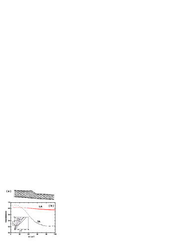
Figure 1: (a) Structure of a (11,0) and (8,0) nanotube junction. (b) The energy transition $T_{n}(\omega)$ as a function of angular frequency $\omega$. The inset shows the dispersion relation of the infinite-long (11,0) nanotube.

We first discuss the SBE results of the transmission coefficients for a nanotube junction, shown in Fig. 1. This calculation involves $504$ equations and $455$ variables. The semiconductor nanotube junction structure is optimized by a second-generation Brenner potential dwbrenner with the force constants derived from the same potential. The phonon dispersion for nanotube (11,0) is illustrated in the inset, in which four acoustic branches are considered: the longitudinal mode (LA), doubly degenerate transverse mode (TA), and the unique twist mode (TW) in nanotubes. Although all modes of a given frequency are considered, we did not find mode-mixing behavior among acoustic modes at the lower frequency range. The transmission for LA mode stays around 0.8 with only small changes. This value is below the AM model prediction of $0.98$ with the longitudinal group velocity $20.18\;{\rm km}\!\cdot\!{\rm s}^{-1}$ and $20.95\;{\rm km}\!\cdot\!{\rm s}^{-1}$ for (11,0) and (8,0). In contrast, the transmission for TA mode decreases with frequency. This can be accounted for by a nearly quadratic dispersion relation of the TA mode, as illustrated in the inset. The transmissions of the TW mode and many other optical modes are nearly zero or very small. This appears related to the difference in rotational symmetries of these modes. We propose that this kind of mode-dependent transmission behavior may be important for further application such as phonon filters.

Next, we consider two acoustically mismatched chains of the same atomic mass connected with springs of different stiffnesses $K_{1},K_{2}$ and lattice constants $a,b$ on each side. The energy transmission by transfer matrix calculation is $\left|t\right|^{2}\frac{\widetilde{v}_{R}}{\widetilde{v}_{L}}={4\left({\frac{\widetilde{v}_{R}}{\widetilde{v}_{L}}}\right)^{2}}/{\left({1+\frac{\widetilde{v}_{R}}{\widetilde{v}_{L}}}\right)^{2}}$ where $\widetilde{v}_{L}=v_{L}/a$, $\widetilde{v}_{R}=v_{R}/b$. Using mass densities $\rho_{L}=m/a$, $\rho_{R}=m/b$ and $z_{L}=\rho_{L}v_{L}$, $z_{R}=\rho_{R}v_{R}$, the AM model gives walittle $\frac{4z_{L}z_{R}}{(z_{L}+z_{R})^{2}}={4\left({\frac{\widetilde{v}_{R}}{\widetilde{v}_{L}}}\right)^{2}}/{\left({1+\frac{\widetilde{v}_{R}}{\widetilde{v}_{L}}}\right)^{2}}$, in agreement with our result. Thus, for simple lattice structure and smooth junction, the results of LD and AM are the same.

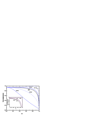
Figure 2: Energy transmission $T(\omega)$ as a function of scaled angular frequency $\omega/\sqrt{4K_{1}}$. Different curves correspond to different coupling strength ratios $\gamma=K_{f}/K_{1}$ at the junction with the spring stiffness parameters $K_{2}=2.6K_{1}$. The inset shows the difference in the prediction of energy transmission for the composite lattice structure, $K_{2}=0.3846K_{1}$, $K_{3}=K_{1}$ for AM-1 and LD-1; $K_{2}=1.1538K_{1}$, $K_{3}=3.0K_{1}$ for AM-2 and LD-2.

For a more realistic model, not only the physical lattice may be composite, but also the boundaries can be more complex. We choose effective stiffness to fit the diamond structure Silicon (Si) and Germanium (Ge) phonon dispersion relations. For Si and Ge along the direction $\Gamma$-$X$, the highest frequency for acoustic phonon branch is about $400\;{\rm cm}^{-1}$ and $250\;{\rm cm}^{-1}$, respectively giannozzi . If the phonon dispersion relation along this direction can be regarded as one-dimensional phyldgaard , the spring stiffness for each can be calculated by $\omega=\sqrt{4k/m}=\sqrt{4K}$. We use these experimental parameters $K_{2}=2.6K_{1}$ for Si and Ge in the following discussion.

Fig. 2 shows how the energy transmission changes with the boundary spring stiffness $K_{f}$. It is reasonable to assume that the stiffness $K_{f}$ for the Si-Ge junction is between pure Si and Ge lattices. When $\gamma=K_{f}/K_{1}=1.5$ or 2.3, the transmission is higher than the prediction given by direct acoustic mismatch model. Moreover, when the lattice structure is not a simple lattice, we also find that AM model does not hold any more. The inset in Fig. 2 shows the discrepancy in the prediction of the energy transmission by AM and LD model for a simple lattice with stiffness $K_{1}$ on the left and alternating stiffness $K_{2}$ and $K_{3}$ on the right. Comparing with LD result, the prediction of AM model overestimates the energy transmission at high frequency for mismatched composite lattice structure.

Figure 3: Energy transmission $T(\omega)$ of a superlattice with the Si and Ge leads; $\omega$ is scaled by $\sqrt{4K_{1}}$. (a) Superlattice of alternating Si and Ge monolayer, $n$ is the number of periods. (b) Superlattice of ten period layers, each layer with $5\times 5$ Si and Ge monolayers.

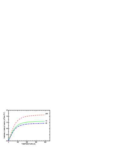
Figure 4: Thermal conductance as a function of temperature. Curves labeled $10$ and $40$ represent ten superlattice period layers, each layer with $5\times 5$ and $20\times 20$ Si and Ge monolayers, respectively; For comparison, the acoustic mismatch (AM) model result of a single Si-Ge interface is also plotted.

Furthermore, when the interfaces are made of periodical superlattices of Si and Ge, interesting phenomenon emerges. Fig. 3$(a)$ shows a series of peaks appearing in the transmission for the superlattice of alternating Si and Ge monolayer. We find that this behavior can be understood as a resonance effect. This kind of resonant tunneling transmission has been reported in phyldgaard . When the superlattice layer is composed of several monolayers of Si and Ge, normal mode calculation shows that resonant frequencies fall into different parts and band gaps are brought about by the repetition of superlattice structure. So it can be seen that the total energy transmission is the acoustic mismatch transmission modulated by the resonance.

We find that these resonance gaps will relate the thermal conductance of superlattice with the thickness of the period layer. We map the 1D chain results to a 3D lattice using an average lattice constant $l_{0}=5.5\;$Å for the cross section of the cell, and 8 chains per conventional diamond-type cell. Our result of thermal conductance is given as $G\approx 10^{9}\;{\rm Wm}^{-2}{\rm K}^{-1}$ at $200\,$K, which agrees quantitatively with the measured effective values in selee . From Fig. 4, we see that thermal conductance decreases with the increase in the thickness of period $L$ at high temperatures ($>100\,$K) due to the appearance of mini gaps in the transmission, which agrees with the experimental result in selee . We argue that in the several superlattice length scale the thermal conductance is wave-natured ballistic transport because the phonon mean free path is comparable to this length scale. But for the samples of thickness of order $\mu$m selee , the total thermal resistance will be the diffusive summation of the microscopic ballistic thermal resistance because wave coherence will be destroyed after transporting across a few superlattice periods. So the effective thermal conductance in selee will exhibit microscopic ballistic thermal transport behavior. Authors of Ref superlattice interpret this kind of thermal conductance as “partially coherent heat conduction” by introducing an imaginary wave vector. When the thickness of the superlattice is larger than the phonon mean free path, the conventional diffusive conductance comes into play and the thermal conductivity will rise with increasing $L$ selee . These qualitative agreements between our calculations and the experimental results suggest a ballistic heat transport as the dominating mechanism within a few superlattice periods. Another feature we find from our calculation is that for lower temperatures ($<50\,$K), the superlattice conductance becomes independent of the thickness and tends to some universal value. We expect that some experiments will verify this point in future.

In summary, we have derived a Landauer formula suitable for lattice dynamic calculations. The transmission coefficients are calculated by a linear equation solver with proper boundary conditions. We have applied our methods to two types of junction structures, and give significant results.

We thank Ming Tze Ong and Nan Zeng for critical readings of the manuscript. This work is supported in part by a Faculty Research Grant of National University of Singapore.

References

- (1) A. Balandin and K. L. Wang, Phys. Rev. B 58, 1544 (1998); Q. F. Sun, P. Yang, and H. Guo, Phys. Rev. Lett. 89, 175901 (2002); B. Li, L. Wang, and G. Casati, Phys. Rev. Lett. 93, 184301 (2004).
- (2) S. Lepri, R. Livi, and A. Politi, Phys. Rep. 377, 1 (2003). J.-S. Wang and B. Li, Phys. Rev. Lett. 92, 074302 (2004).
- (3) K. Schwab et al., Nature 404, 974 (2000).
- (4) D. G. Cahill et al., J. Appl. Phys. 93, 793 (2003).
- (5) E. T. Swartz and R. O. Pohl, Rev. Mod. Phys. 61, 605 (1989); P. L. Kapitza, J. Phys. (Moscow) 4, 181 (1941).
- (6) C. L. Tien and G. Chen, J. Heat Transfer, 116, 799 (1994); G. Chen, Phys. Rev. B 57, 14958 (1998).
- (7) B.C. Daly et al., Phys. Rev. B 66, 024301 (2002).
- (8) D. A. Young and H. J. Maris, Phys. Rev. B 40, 3685 (1989).
- (9) L. G. Rego and G. Kirczenow, Phys. Rev. Lett. 81, 232 (1998); M. P. Blencowe, Phys. Rev. B 59, 4992 (1999).
- (10) L. Kantorovich, Quantum Theory of the Solid State: an Introduction, p.141 (Kluwer Academic Publishers, 2004).
- (11) D. W. Brenner et al., J. Phys.: Condens. Matter. 14, 783 (2002).
- (12) W. A. Little, Can. J. Phys. 37, 334 (1959).
- (13) P. Giannozzi et al., Phy. Rev. B 43, 7231 (1991).
- (14) P. Hyldgaard, Phys. Rev. B 69, 193305 (2004).
- (15) S.-M. Lee, D. G. Cahill, and R. Venkatasubramanian, Appl. Phys. Lett. 70, 2957 (1997); S. Chakraborty et al., Appl. Phys. Lett. 83, 4184 (2003).
- (16) M. V. Simkin and G. D. Mahan, Phys. Rev. Lett. 84, 927 (2000); B. Yang and G. Chen, Phys. Rev. B 67, 195311 (2003).