The continuum gauge field-theory model for low-energy electronic states of icosahedral fullerenes

Abstract

The low-energy electronic structure of icosahedral fullerenes is studied within the field-theory model. In the field model, the pentagonal rings in the fullerene are simulated by two kinds of gauge fields. The first one, non-abelian field, follows from so-called K spin rotation invariance for the spinor field while the second one describes the elastic flow due to pentagonal apical disclinations. For fullerene molecule, these fluxes are taken into account by introducing an effective field due to magnetic monopole placed at the center of a sphere. Additionally, the spherical geometry of the fullerene is incorporated via the spin connection term. The exact analytical solution of the problem (both for the eigenfunctions and the energy spectrum) is found.
PACS: 73.22.-f

I Introduction

The electronic structure and elementary excitations of
fullerene molecules have been of steady interest since the discovery of the first so-called buckminsterfullerene C₆₀ [1] because the knowledge of the electronic structure gives an important information about the electric and photo conductivity, magnetic behavior, etc. All these characteristics were found to be rather unique in fullerene molecules (see, e.g., review [2]), which can be effectively used in some practical applications in devices based on fullerenes.

There is a number of different theories to study this problem, which can be roughly divided into three general groups. The first one includes empirical methods like the free-electron gas [3], and tight-binding [4, 5, 6, 7] calculations. The second one uses ab initio quantum chemistry calculations [8]. The third group considers the continuum models within the effective-mass description [9, 10, 11].

While the continuum description is limited to the electronic states close to the Fermi level, it has some interesting attractive features. First of all it gives a possibility to study large fullerenes where the numerical analysis is a rather difficult task. Second, it reveals the long-distance physics which is of importance in various carbon nanoparticles. Finally, the continuum description allows to elucidate ”true” topological effects like the appearance of the Aharonov-Bohm phase and anomalous Landau levels due to disclinations.

In this paper, we formulate a continuum model to study low-energy electron states in icosahedral fullerenes. The model is a variant of the effective field theory on a sphere describing Dirac wavefunctions interacting with two types of gauge fluxes. One of the fluxes is due to so-called $K$ spin rotation invariance (see [12] for details) and the second one comes from the local SO(2) invariance of the two-dimensional elastic Lagrangian in the presence of disclinations [13]. Actually, the second flux describes the elastic flow through a surface due to a disclination and has a topological origin (its circulation is determined by the Frank index, the topological characteristic of the defect). For this reason, this flux exists even within the so-called ”inextensional” limit (which is usually adjusted to fullerene molecule [14]). Notice that the topological origin the elastic flux results in appearance of the disclination-induced Aharonov-Bohm-like phase (see [15]).

It should be mentioned that the first continuum model for the description of fullerene molecule was presented in two papers [9, 10]. A different variant of the continuum model for fullerene was suggested in [11]. The first model neglected the topological origin of the disclination defects while the second model missed the $K$ spin rotation invariance. However, in both papers the non-trivial zero-mode electronic states are considered. In this paper we found an exact analytical solution of the problem at low energies.

II General formalism

Let us start from the standard formalism based on the effective-mass theory proposed in [16] to study the screening of a single intercalant within a graphite host. A graphite host is considered as a single graphite plane (graphene). Actually, the effective-mass expansion is equivalent to the $\vec{k}\cdot\vec{p}$ expansion of the graphite energy bands about the $\vec{K}$ point in the Brillouin zone when the intercalant potential is zero. In fact, there are two degenerate Bloch eigenstates at $\vec{K}$, so that the microscopic wave function can be approximated by

$$\Psi(\vec{k},\vec{r})=f_{1}(\vec{k}^{\prime})e^{i\vec{k}^{\prime}\vec{r}}\Psi^{S}_{1}(\vec{K},\vec{r})+f_{2}(\vec{k}^{\prime})e^{i\vec{k}^{\prime}\vec{r}}\Psi^{S}_{2}(\vec{K},\vec{r})$$ (1)

where $\vec{k}=\vec{K}+\vec{k^{\prime}}$. Keeping terms of order $\vec{k}^{\prime}$ in the Schrödinger equation one can obtain the secular equation for functions $f_{1,2}(\vec{k}^{\prime})$ and after diagonalization one finally gets the two-dimensional Dirac equation (see  [16] for details)

$$-i\sigma^{\mu}\partial_{\mu}\psi(\vec{r})=E\psi(\vec{r})$$ (2)

where $\sigma^{\mu}$ are the conventional Pauli matrices ($\mu=1,2$), the energy $E$ is accounted from the Fermi energy, the Fermi velocity $V_{F}$ is taken to be one, and the two-component wave function $\psi$ represents two graphite sublattices ($A$ and $B$). As was mentioned in [16] the essence of the $\vec{k}\cdot\vec{p}$ approximation is to replace the graphite bands by conical dispersions at the Fermi energy. In addition, one has to take into account two independent wave vectors ($\vec{K}_{+}=\vec{K}$ and $\vec{K}_{-}=-\vec{K}$) in the carbon lattice which give the same conical dispersion. Therefore, the states $\mid\vec{K}_{\pm}A>$ and $\mid\vec{K}_{\pm}B>$ can be chosen as the full basis set  [12].

For our purpose, to take into account both the spherical geometry of a fullerene molecule and disclinations on its surface we have to modify the model (2) by introducing three additional fields.

A The compensating fields

As a first step, let us consider a single disclination in a graphene sheet. To introduce the fivefold in the hexagonal lattice one has to cut the sector $2\pi/6$ and glue the opposite sides ($OB$ and $OB^{\prime}$ in Fig.1).

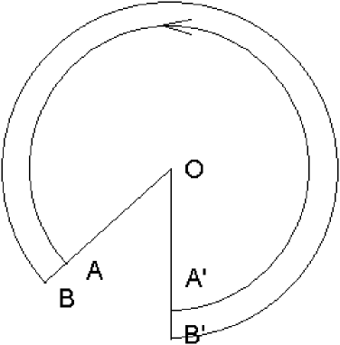
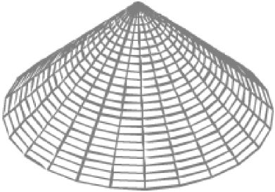
FIG. 1.: A disclination in elastic membrane (right) and the image of the membrane (left).

Notice that this is a typical cut-and-glue procedure to incorporate a disclination in an elastic plane. There exist several continuum theories for the description of disclinations in flexible membranes (see [13, 17, 18]) which allow to formulate similar von Karman equations. In the ”inextensional” limit (free to bend, impossible to stretch), the exact solution for an isolated positive disclination was found in [17]. It was shown that the elastic membrane becomes buckled and takes a conical form (see Fig.1). For our purpose, the most appropriate is the gauge theory of disclinations on fluctuating elastic surfaces formulated in [13]. Indeed, this is the most convenient theory to take into account the topological origin of the disclination defect. The elastic flux due to pentagonal apical disclination represented by abelian gauge field $\vec{W}$ is given by (see [11, 15])

$$\oint W_{\mu}dx^{\mu}=\frac{2\pi}{6}.$$ (3)

As is seen, the elastic flux for pentagonal defect is exactly $1/6$. It was shown in [15] that the electronic eigenfunction acquires the additional Aharonov-Bohm-like phase due to nontrivial topology of elastic surface with a disclination vortex. In our case, this phase will appear both in the Bloch (1) and the Dirac (2) wavefunctions.

To exclude the discontinuous boundary conditions for spinor fields on the sector sides (lines $OB$ and $OB^{\prime}$ on Fig.1) let us introduce two additional fields. First, constructing a boundary condition for the spinor components on the line $OB\equiv OB^{\prime}$ one has to take into account the exchange between A and B sublattices which takes place for the sector angle $\pi/3$. This can be done by using an appropriate boundary condition for the K spin part in the form (see [12])

$$\psi(\varphi+2\pi)=-T\psi(\varphi),\quad T=i\tau_{2}=\exp(i\frac{\pi}{2}\tau_{2})$$ (4)

where the Pauli matrix $\tau_{2}$ acts on the K part of the spinor components, and $\varphi$ is the polar coordinate on the membrane ($0\leq\varphi<2\pi$). One can introduce the non-Abelian gauge field $\vec{a}$ to eliminate the exponential factor. In this case, the circulation of the field $\vec{a}$ is written as [12]

$$\oint a_{\mu}dx^{\mu}=\tau_{2}\frac{2\pi}{4}.$$ (5)

As is seen, this field adds $\pm 1/4$ to the total flux. It should be mentioned that the circulation of the gauge field $\vec{a}$ is governed by topology of the lattice and does not depend upon geometry of the structure. Thus these operators and fluxes can be obtained solely from the lattice structure.

The last field to be introduced is the frame rotation field $\vec{Q}$ which is equivalent to the spin connection (see [12]). This field (analog to the metrical connection coefficients) rotates the frame by the angle $2\pi/6$, and its circulation along the contour $A^{\prime}A$ is determined by the following condition:

$$\oint Q_{\mu}dx^{\mu}=-\sigma_{3}\frac{\pi}{6}.$$ (6)

Notice that the spin connection does not contribute to the total flux.

B The covariant description and the Dirac equation on the curved surface

So far we considered the problem on the plane by using the discontinuous planar coordinates (with the borders of the sector OB and OB^′). Instead, one can also use the continuous coordinates on the Riemannian surface $\vec{r}(r,\varphi)$, $0\leq\varphi<2\pi$ (see Fig.1). To incorporate fermions on the curved background we need a set of orthonormal frames $\{e_{\alpha}\}$ which yield the same metric, $g_{\mu\nu}$, related to each other by the local $SO(2)$ rotation,

$$e_{\alpha}\to e^{\prime}_{\alpha}={\Lambda}_{\alpha}^{\beta}e_{\beta},\quad{\Lambda}_{\alpha}^{\beta}\in SO(2).$$

It then follows that $g_{\mu\nu}=e^{\alpha}_{\mu}e^{\beta}_{\nu}\delta_{\alpha\beta}$ where $e_{\alpha}^{\mu}$ is the zweibein, with the orthonormal frame indices being $\alpha,\beta=\{1,2\}$, and coordinate indices $\mu,\nu=\{1,2\}$. As usual, to ensure that physical observables are independent of a particular choice of the zweibein fields, a local $so(2)$-valued gauge field $\omega_{\mu}$ must be introduced. The gauge field of the local Lorentz group is known as the spin connection. For the theory to be self-consistent, the zweibein fields must be chosen to be covariantly constant [20],

$${\cal D}_{\mu}e^{\alpha}_{\nu}=\partial_{\mu}e^{\alpha}_{\nu}-\Gamma^{\lambda}_{\mu\nu}e^{\alpha}_{\lambda}+(\omega_{\mu})^{\alpha}_{\beta}e^{\beta}_{\nu}=0,$$

which determines the spin connection coefficients explicitly

$$(\omega_{\mu})^{\alpha\beta}=e_{\nu}^{\alpha}D_{\mu}e^{\beta\nu}.$$ (7)

Finally, the Dirac equation (2) on a surface $\Sigma$ in presence of the $U(1)$ external gauge field $W_{\mu}$ and the gauge field $a_{\mu}$ is written as

$$i\gamma^{\alpha}e_{\alpha}^{\ \mu}(\nabla_{\mu}-ia_{\mu}-iW_{\mu})\psi=E\psi,$$ (8)

where $\nabla_{\mu}=\partial_{\mu}+\Omega_{\mu}$ with

$$\Omega_{\mu}=\frac{1}{8}\omega^{\alpha\ \beta}_{\ \mu}[\gamma_{\alpha},\gamma_{\beta}]$$ (9)

being the spin connection term in the spinor representation. Notice that $\Omega_{\mu}=-i{Q}_{\mu}$ which justifies the above-mentioned relation between the frame rotation field and the spin connection. The spinor in (8) has the form $\psi=(F_{A}^{K}\;F_{B}^{K}\;F_{A}^{K_{-}}\;F_{B}^{K_{-}})^{T}$ where $F(\vec{r})$ are envelope functions,

$$\gamma_{\alpha}=-I\,\sigma_{\alpha}=-\left(\begin{array}[]{cc}\sigma_{\alpha}&0\\ 0&\sigma_{\alpha}\end{array}\right),\;\oint a_{\mu}dx^{\mu}=\frac{2\pi}{4}\tau_{2}I=\frac{2\pi}{4}\left(\begin{array}[]{cc}0&-i\,I\\ i\,I&0\end{array}\right).$$ (14)

The matrix $\tau_{2}$ acting in K-spin space appears in (8) only through $a_{\mu}$. Therefore (8) can be easily diagonalized and we arrive at the two-component Dirac equations in the form

$$-i\sigma^{\alpha}e_{\alpha}^{\ \mu}(\nabla_{\mu}-ia_{\mu}^{k}-iW_{\mu})\psi^{k}=E\psi^{k}.$$ (15)

As is seen, the coupled pair of equations (8) is reduced to the decoupled one describing ”K-spin up” ($K^{\uparrow}$) and ”K-spin down” ($K^{\downarrow}$) states. The field $a_{\mu}^{k}$ is determined by a condition

$$\oint a_{\mu}^{k}dx^{\mu}=\pm\frac{2\pi}{4},$$

with the sign plus (minus) taken for $k=K^{\uparrow}$ ($k=K^{\downarrow}$), respectively. Notice that after diagonalization the four-component spinor $\psi$ is found to be decomposed into ”upper” and ”lower” doublet components, $\psi^{K^{\uparrow}}$ and $\psi^{K^{\downarrow}}$, each of them transforms via SU(2).

C The continuum model for the icosahedral fullerene

According to the Euler’s theorem, the fullerene molecule consists of exactly twelve disclinations. Generally, it is difficult to take into account properly all the disclinations. There are two ways to simplify the problem. First, one can consider a situation near a single defect (similar to [11]) taking into account that each defect in the fullerene can be simulated by two fluxes: K spin flux (5) and the elastic flux (3). In the case of sphere, however, the most appropriate approximation is to introduce the effective field replacing the fields of twelve disclinations by the field of the magnetic ’t Hooft-Polyakov monopole with a constant flux density and the half-integer charge $A$ [10].

The total flux of the monopole $4\pi A$ is equal to the sum of fluxes from all the disclinations. The procedure of summing up non-abelian fictitious fluxes from apical defects placed at different points of the graphite cones was presented in [12] (so-called $"n-m"$ combination rule). Namely, for the field $\vec{a}$ a linear integral circulating any even number of defects on the lattice is determined by $\tau_{3}\,(N\pi/2-(2\pi/3)[(n-m)\,$ (mod $3)])$, where $N$ is a number of defects, n and m are numbers of steps in positive and negative directions, respectively (see [12]). The directions rotated by $2\pi/3$ are considered to be identical. This gives a natural $(n,m)$ classification of two-pentagon lattices: those for which $n\equiv m$ (mod 3), and those for which $n\neq m$ (mod 3). This approach is suitable for the case of a sphere.

As is shown below, the eigenfunctions of the low-energy levels oscillate not too fast with a distance, therefore the effective ”monopole-like” approximation is valid for small quantum numbers (and near the Fermi energy). So, one can introduce the continuous field created by the ’t Hooft-Polyakov monopole placed at the center of the sphere. In this case, the contour of integration is represented by two circles around the poles of the sphere as shown in Fig.2.

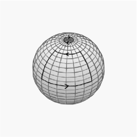
FIG. 2.: The integration path on the sphere. The path shown at the center encircles a few fivefolds. The ”total” path of the integration, encircling all twelve pentagons, includes two contours around the poles: negatively directed for the north pole (shown) and positively directed for the south pole (not shown).

Notice that for fullerenes with the full icosahedral symmetry (Ih) the combined flux turns out to be a sum of fluxes due to any pair of defects. Thus, the combined flux does not depend upon the arrangement of pentagons because any corresponding fragment of the lattice turns out to be of the above-mentioned class $(1,1)$. In other words, in icosahedral fullerenes $(n-m)$  (mod 3) = 0 due to the mirror symmetry of the lattice. Finally, the continuous fields take the form

$$a^{k}_{\theta}=0,a^{k}_{\varphi}=\pm\frac{3}{2}\cos\theta,\quad W_{\theta}=0,W_{\varphi}=-\cos\theta.$$

It should be noted that for the Dirac field in the external potential provided by a monopole, the effective ”charge” $A$ involves the ”isospin” matrix $\tau^{\prime}$ (see [21]). This matrix can be also diagonalized in the Dirac equation thus giving the additional sign $\pm$ to the whole charge. What is important, the coordinate behavior of this field is the same as for the spin connection field (cf. [22, 10]). This fact allows us to find the exact analytical solution of the problem. Another significant fact is the presence of ”isospin” matrix in the momentum operator. Similarly to [10]

$$J_{z}=-i(\nabla_{\varphi}-iA{\tau}_{2}^{\prime}\cos\theta)+\frac{{\sigma}_{z}}{2}\cos\theta+A\cos\theta{\tau}_{2}^{\prime}$$ (16)

and for half-integer $A$ this operator takes integer eigenvalues $j=0,\pm 1,\pm 2,...$.

III The electronic states of the fullerene

In accordance with the results of the previous section, the total ”charge” is written as $A=\pm(a^{k}_{\varphi}+W_{\varphi})/\cos\theta=\pm 1/2,\pm 5/2$. Therefore, the Dirac operator in (8) takes the following form:

$$\hat{\cal{D}}=-i\sigma_{x}(\partial_{\theta}+\frac{\cot{\theta}}{2})-i\frac{\sigma_{y}}{\sin\theta}(\partial_{\varphi}-iA\cos\theta).$$

The substitution

$$\left(\begin{array}[]{c}\psi_{A}\\ \psi_{B}\\ \end{array}\right)=\sum_{j}\frac{e^{ij\varphi}}{\sqrt{2\pi}}\left(\begin{array}[]{c}u_{j}(\theta)\\ v_{j}(\theta)\\ \end{array}\right),j=0,\pm 1,\pm 2,\ldots$$

leads to the equations for $u_{j}$ and $v_{j}$

$$-i(\partial_{\theta}+[\frac{1}{2}-A]\cot\theta+\frac{j}{\sin\theta})v_{j}(\theta)=Eu_{j}(\theta),$$ (17)

$$-i(\partial_{\theta}+[\frac{1}{2}+A]\cot\theta-\frac{j}{\sin\theta})u_{j}(\theta)=Ev_{j}(\theta).$$ (18)

The square of the Dirac operator reads

$${\hat{\cal{D}}}^{2}=-[\sigma_{x}(\partial_{\theta}+\frac{\cot{\theta}}{2})+i\frac{\sigma_{y}}{\sin\theta}(j-A\cos\theta)]^{2}=$$ (19)

$$=-\frac{1}{\sin\theta}\partial_{\theta}\sin\theta\partial_{\theta}+\frac{1}{4}+\frac{\frac{1}{4}+j^{2}+\sigma_{z}A}{\sin^{2}\theta}-\frac{\cot\theta}{\sin\theta}(\sigma_{z}j+2jA)+A^{2}\cot^{2}\theta.$$ (20)

Let us write the equation $\hat{\cal{D}}^{2}\psi=E^{2}\psi$ by using the appropriate substitution $x=\cos\theta$. From (20) one obtains

$$\left[\partial_{x}(1-x^{2})\partial_{x}-\frac{(j-Ax)^{2}-j\sigma_{z}x+\frac{1}{4}+\sigma_{z}A}{1-x^{2}}\right]\left(\begin{array}[]{c}u_{j}(x)\\ v_{j}(x)\\ \end{array}\right)=-(E^{2}-\frac{1}{4})\left(\begin{array}[]{c}u_{j}(x)\\ v_{j}(x)\\ \end{array}\right)$$ (25)

Taking into account the asymptotic behavior of the spinor functions, one can use the substitution

$$\left(\begin{array}[]{c}u_{j}\\ v_{j}\\ \end{array}\right)=\left(\begin{array}[]{c}(1-x)^{\alpha}(1+x)^{\beta}{\tilde{u}}_{j}(x)\\ (1-x)^{\gamma}(1+x)^{\delta}{\tilde{v}}_{j}(x)\\ \end{array}\right),$$

where

$$\alpha=\frac{1}{2}\left|j-A-\frac{1}{2}\right|,\quad\gamma=\frac{1}{2}\left|j-A+\frac{1}{2}\right|$$ (26)

$$\beta=\frac{1}{2}\left|j+A+\frac{1}{2}\right|,\quad\delta=\frac{1}{2}\left|j+A-\frac{1}{2}\right|$$ (27)

Then the equation (25) for the function ${\tilde{u}}_{j}$ takes the form

$$(1-x^{2})\partial_{x}^{2}{\tilde{u}}_{j}+(2(\beta-\alpha)-2(\alpha+\beta+1)x)\partial_{x}{\tilde{u}}_{j}+[-2\alpha\beta-\alpha-\beta-\frac{1}{2}(j^{2}-A^{2}+\frac{1}{4}-A)+E^{2}-\frac{1}{4}]{\tilde{u}}_{j}=0.$$ (28)

This is equivalent to the Jacobi equation

$$(1-x^{2})y^{\prime\prime}+({\cal{B}}-{\cal{A}}-({\cal{A}}+{\cal{B}}+2)x)y^{\prime}+\lambda_{n}y=0,$$ (29)

$$\lambda_{n}=n(n+{\cal{A}}+{\cal{B}}+1),$$ (30)

with ${\cal{A}}=2\alpha,\,{\cal{B}}=2\beta$, and $n$ being any non-negative integer. In view of (28) and (30) one gets the quantization condition

$$\lambda_{n}=n(n+2(\alpha+\beta)+1)=-2\alpha\beta-\alpha-\beta-\frac{1}{2}(j^{2}-A^{2}+\frac{1}{4}-A)+E^{2}-\frac{1}{4}.$$ (31)

Taking into account (27), one obtains the energy spectrum in the form $E_{n}^{2}=(n+\alpha+\beta+1/2)^{2}-A^{2}$. When $A=0$, one has $\alpha=(1/2)|j-1/2|,\,\beta=(1/2)|j+1/2|$ and the energy spectrum is identical to the one found in [22] for the Riemann sphere without a monopole.

In a similar manner one can study the equation for the function $\tilde{v}$. This gives another energy spectrum $E_{n}^{2}=(n+\gamma+\delta+\frac{1}{2})^{2}-A^{2}$. It should be mentioned that both solutions (for $\tilde{u}$ and $\tilde{v}$) should satisfy (18). This is possible if the condition $\alpha+\beta=\gamma+\delta$ holds true and, on the other hand, if one of the energies in the equations for $u$ and $v$ becomes zero.

Let us consider the first case. The possible values of $j$ are found to be $|j|\geq||A|+1/2|$. For $E>0$ one obtains the spectrum

$$E_{n}^{2}=(n+|j|+1/2)^{2}-A^{2},\\$$ (32)

and the eigenfunctions

$$u_{j}=C_{u}(1-x)^{\alpha}(1+x)^{\beta}P_{n}^{2\alpha,2\beta},$$ (33)

$$v_{j}=C_{v}(1-x)^{\gamma}(1+x)^{\delta}P_{n}^{2\gamma,2\delta},$$ (34)

$P_{n}$ are the Jacobi polynomials. The unit of energy here is $\hbar V_{F}/R$ where $R$ is the fullerene radius. One should note that (32) is not allowed for analysis of zero-mode states. In particular, the degeneracy of the zero-mode state can not be calculated using (32). According to (18), the factors $C_{u}$ and $C_{v}$ in (34) are interrelated. Indeed, for $j>0$ one has

$$i[(1-x^{2})\partial_{x}-2\gamma-2\beta x]C_{v}P_{n}^{2\gamma,2\beta-1}=E_{n}(1+x)C_{u}P_{n}^{2\gamma-1,2\beta},$$ (35)

$$i[(1-x^{2})\partial_{x}+2\beta-2\gamma x]C_{u}P_{n}^{2\gamma-1,2\beta}=E_{n}(1-x)C_{v}P_{n}^{2\gamma,2\beta-1}.$$ (36)

Setting $x=1$ in the first equation and using the definition

$$P_{n}^{a,b}(1)=\frac{\Gamma(a+n+1)}{\Gamma(a+1)n!},\quad E_{n}=\pm\sqrt{(2\gamma+n)(2\beta+n)},$$

one finally gets for $j>0$

$$C_{u}=-iC_{v}\mathop{\mathrm{sign}}\nolimits{E_{n}}\left(\frac{j+1/2}{j+1/2-A}\right)\left(\frac{n+j-A+1/2}{n+j+A+1/2}\right)^{1/2}$$ (37)

In general case, for arbitrary signs of $E$ and $j$, we obtain

$$C_{u}=-iC_{v}\mathop{\mathrm{sign}}\nolimits{(jE_{n})}\left(\frac{|j|+1/2}{|j|+1/2-A\mathop{\mathrm{sign}}\nolimits j}\right)^{\mathop{\mathrm{sign}}\nolimits j}\left(\frac{n+|j|-A+1/2}{n+|j|+A+1/2}\right)^{1/2}$$ (38)

In the second case, the possible values of $j$ and $n$ are determined by $|j|\leq||A|-1/2|$, $n=0$. One gets exactly one zero-mode at fixed $j$ and positive fixed $A$

$$u_{0}=0,\quad v_{0}=C_{v}(1-x)^{\gamma}(1+x)^{\delta},$$ (39)

where the relation $P_{0}^{2\gamma,2\delta}(x)=const$ is taken into account. Accordingly, if $A<0$ there exists only one zero-mode solution $u_{0}$. Thus, for all possible values of $j$ and all possible positive values of $A$ there exists exactly six different zero-mode solutions $v_{0}$.

It should be noted that both in (34) and in (39) the replacement $j\rightarrow-j,\,A\rightarrow-A$ is equivalent to the exchange $u\rightarrow v,\,v\rightarrow u$ (cf. (18)). This means that ”isospin up” and ”isospin down” components of the spinor on a sphere turns out to be physically equivalent up to the redefinition of the quantum number $j$ and a unitary transformation. Therefore, one can restrict consideration to either component, for instance, to ”isospin up”.

From (32) and (39) one can calculate the energy spectrum. The possible ”charges” are $A=-1/2,5/2$, so that the first four levels are (in units of $\hbar V_{F}/R$) the following: $E=0,1.41,2.45,3.46$. Their degeneracies are $g=6,2,6,6$, respectively. It is interesting to compare these results with tight-binding calculations. However, two preliminary remarks should be done. First, the continuum model is correct for the low-lying electronic states. Second, the validity of the effective field approximation for the description of big fullerenes is not clear yet. In fact, the essence of this approximation is to take into account the isotropic part of long-range defect fields. Probably, for bigger fullerenes both the anisotropic part of the long-range fields and the influence of the short-range fields due to single disclinations should be properly involved. Therefore, the exact values of the energy levels do not agree well with those presented in [4, 5, 6, 7]. At the same time, we can surely verify both the existence of quasi-zero modes found for spherical fullerenes in [4, 5, 6, 7] and their 6-fold degeneracy. There is also a good qualitative agreement in observed scaling of the energy gap between the highest occupied and lowest unoccupied energy levels with the size of the fullerene.

IV Conclusion

In this paper, we have studied the electronic states of the icosahedral fullerene within the continuum field-theory approach. The influence of the disclinations is taken into account by introducing an effective field due to magnetic monopole placed at the center of a sphere and having a total ”charge” $A$. The flux due to monopole is a sum of two fluxes: (i) the K-spin flux and (ii) the elastic flux due to nontrivial topology of the surface with a disclination (the pricked out point on the surface). An exact analytical solution of the problem is found and the explicit form of the zero-energy modes as well as of the energy spectrum is presented.

It should be noted that our approach differs from previous studies of fullerene molecules within the continuum models [9, 10, 11, 23]. The effective monopole field introduced in [9] is identical with the K-spin field $a_{\mu}$. Notice that a similar to [9] monopole field was used in the continuum model of the spheroidal fullerenes [23]. Neither in [9, 10] nor in [23] the analytical solution was found. The presented model differs also from [11] where the gauge field due to K spin was neglected and only one disclination on a sphere was described.

Introducing the gauge field due to elastic vortex we obtain some principally new results. First of all, the effective monopole charge $A$ takes two different values within the proposed model ($-1/2$ and $5/2$) rather than $\pm 3/2$ for icosahedral fullerenes in [9]. In turn, this finding affects the energy spectrum which is a combination of spectra for these two charges. Besides, the eigenfunctions are characterized by different from [10] conditions for the momentum $j$.

Notice that the more precise description of the fullerenes requires inclusion of the electron-phonon interaction. In the simplest form, the role of this interaction was considered in [9]. It was shown that the energy levels become shifted and lose a symmetry around the Fermi level. The similar effect is expected in our model. An interesting open question is the electronic structure of other (non-Ih) types of spherical fullerenes as well as of non-spherical (e.g. elliptical) ones. Probably, the introduction of the monopole-like fields will be also a good approximation, at least for the low-energy states.

We would like to acknowledge M. Pudlak and S. Sergeenkov for useful discussions and comments. This work has been supported by the Russian Foundation for Basic Research under grant No. 05-02-17721.

REFERENCES

- [1] H.W. Kroto, J.R. Heath, S.C. O’Brian, R.F. Curl and R.E. Smalley, Nature 318, 162 (1985).
- [2] G. Gensterblum, J. of Electron Spectroscopy and Related Phenomena, 81, 89 (1996).
- [3] G.A. Gallup, Chem.Phys.Lett., 187, 187 (1991).
- [4] E. Manousakis, Phys. Rev. B 44, 10991 (1991).
- [5] Y.-L. Lin and F. Nori, Phys. Rev. B 49, 5020 (1994).
- [6] A. C. Tang, F. Q. Huang and R. Z. Liu, Phys. Rev. B 53, 7442 (1996).
- [7] A. Pérez-Garrido, F. Alhama and D. J. Katada, Chem. Phys. 278, 77 (2002).
- [8] J.W. Mintmire, B.I. Dunlap, D.W. Brenner, R.C. Mowray and C.T. White, Phys. Rev. B 43, 14281 (1991).
- [9] J. González, F. Guinea and M.A.H. Vozmediano, Phys. Rev. Lett. 69, 172 (1992).
- [10] J. González, F. Guinea and M.A.H. Vozmediano, Nucl.Phys. B 406, 771 (1993).
- [11] V. A. Osipov, E. A.Kochetov, and M. Pudlak, JETP 96, 140 (2003).
- [12] P.E. Lammert and V.H. Crespi, Phys. Rev. B 69, 035406 (2004).
- [13] E.A. Kochetov and V.A. Osipov, J.Phys. A: Math.Gen. 32, 1961 (1999).
- [14] J. Tersoff, Phys.Rev. B 46, 15546 (1992).
- [15] V. A. Osipov, Phys. Lett. A 164, 327. (1992).
- [16] D.P. DiVincenzo and E.J. Mele, Phys. Rev. B 29, 1685 (1984).
- [17] H. S. Seung and D.R. Nelson, Phys.Rev. A 38, 1005 (1988).
- [18] J.-M. Park and T. C. Lubensky, Phys.Rev. E 53, 2648 (1996)
- [19] P.E. Lammert and V.H. Crespi, Phys. Rev. Lett. 85, 5190 (2000).
- [20] M.B. Green, J.H. Schwartz, and E. Witten, Superstring theory, (Cambridge 1988), v. 2.
- [21] R. Jackiw and C. Rebbi, Phys. Rev. D 13, 3398 (1976).
- [22] A. A. Abrikosov jr., Int. Journ. of Mod. Phys. A 17, 885 (2002)
- [23] R. Pincak, Phys. Lett. A 340, 267 (2005)