Spin and charge dynamics of the one-dimensional extended Hubbard model

Abstract

We investigate the dynamical spin and charge structure factors and the one-particle spectral function of the one-dimensional extended Hubbard model at half band-filling using the dynamical density-matrix renormalization group method. The influence of the model parameters on these frequency- and momentum-resolved dynamical correlation functions is discussed in detail for the Mott-insulating regime. We find quantitative agreement between our numerical results and experiments for the optical conductivity, resonant inelastic X-ray scattering, neutron scattering, and angle-resolved photoemission spectroscopy in the quasi-one-dimensional Mott insulator SrCuO₂.

I Introduction

The spectral properties of low-dimensional correlated electron systems have attracted a significant amount of interest in recent years. dionys In particular, the energy and momentum resolution of spectroscopic techniques have been greatly improved. These methods now provide plenty of information about the dispersion and intensity of electronic excitations in low-dimensional materials. For instance, the dynamical separation of charge and spin degrees of freedom, which is generic in the theory of quasi-one-dimensional correlated systems, has been observed directly in angle resolved photoemission spectroscopy (ARPES) of strongly anisotropic cuprate compounds. kim ; koi06 From the viewpoint of theory, however, calculating the response functions that are probed in these experiments remains a great challenge and thus a coherent quantitative description of these materials is still lacking.

Few exact analytical results are available for dynamical response functions in itinerant correlated electron systems. In gapless systems dynamical correlation functions can be evaluated analytically with field-theoretical methods in the limit of small excitation energies. voit Gapped systems can also be treated analytically in the weak-coupling limit when the gap is small compared to the electron band-width. grage ; controzzi At finite excitation energies exact analytical results are available in the strong-coupling regime penc-spectral ; pencdensity or when additional symmetries are present. arikawa

There are several numerical approaches for calculating momentum- and frequency-dependent correlation functions in lattice models of correlated electrons. These include Exact Diagonalization, bannister Cluster Perturbation Theory (CPT), senechal Variational CPT, potthoff and Quantum Monte Carlo algorithms. preuss ; lavalle Here we employ the Dynamical Density-Matrix Renormalization Group (DDMRG) method. ddmrg It is a zero-temperature method which has been successfully applied to the study of dynamical properties in metallic and insulating phases of one-dimensional extended Hubbard models. rixs ; hubbard-spectral ; tioclpaper ; diss ; matsueda

In this paper we consider the dynamical properties of the half-filled extended Hubbard model with nearest-neighbor interaction. It is believed to be a minimal model for quasi-one-dimensional Mott-insulators, such as the cuprate compounds SrCuO₂ and Sr₂CuO₃. In a previous work rixs we have shown that this model describes the optical conductivity and the dispersive structures observed in the resonant inelastic x-ray scattering (RIXS) experiments of SrCuO₂. Here we show that the model also captures essential results obtained in inelastic neutron scattering, zaliznyak electron energy loss spectroscopy (EELS), eels and ARPES kim ; koi06 experiments. To this end we present numerical results for the energy- and momentum-resolved spin and charge structure factors and the one-particle spectral function of the extended Hubbard model. We also discuss in detail the influence of the model parameters on the line shapes of structure factors and spectral functions.

II Model and Methods

The one-dimensional extended Hubbard model is defined by the Hamiltonian

$$\hat{H} = -t\sum_{l,\sigma}\left(\hat{c}^{\dagger}_{l,\sigma}\hat{c}^{\phantom{\dagger}}_{l+1,\sigma}+\hat{c}^{\dagger}_{l+1,\sigma}\hat{c}^{\phantom{\dagger}}_{l,\sigma}\right)$$

$$+U\sum_{l}\left(\hat{n}_{l,\uparrow}-\frac{1}{2}\right)\left(\hat{n}_{l,\downarrow}-\frac{1}{2}\right)$$

$$+V\sum_{l}\left(\hat{n}^{\phantom{\dagger}}_{l}-1\right)\left(\hat{n}^{\phantom{\dagger}}_{l+1}-1\right).$$

Here $\hat{c}^{\dagger}_{l,\sigma}$, $\hat{c}^{\phantom{\dagger}}_{l,\sigma}$ are fermionic creation and annihilation operators for a particle with spin $\sigma=\uparrow,\downarrow$ at site $l=1,\dots,L$, $\hat{n}^{\phantom{\dagger}}_{l,\sigma}=\hat{c}^{\dagger}_{l,\sigma}\hat{c}^{\phantom{\dagger}}_{l,\sigma}$, and $\hat{n}^{\phantom{\dagger}}_{l}=\hat{n}^{\phantom{\dagger}}_{l,\uparrow}+\hat{n}^{\phantom{\dagger}}_{l,\downarrow}$. In the following we consider chains with open boundary conditions and an even number of lattice sites. The total number of electrons is equal to the number of lattice sites (half-filled band).

For $V/t=0$ the model reduces to the simple Hubbard Hamiltonian. Without magnetic field the physical excitations of the insulating Hubbard model are combinations of collective modes, spinons and (anti-)holons, for any $U>0$. theBook The spinons are gapless and charge neutral excitations that carry spin $1/2$. Anti-holons and holons are gapped modes with charge $\pm e$ and no spin. When the nearest-neighbor interaction $V$ is turned on and $U>0$, the system remains a Mott-insulator until $V\approx U/2$. For larger $V$ the system becomes a charge-density wave (CDW) insulator. eric-ehm In this work we only consider the Mott-insulating regime $U>2V\geq 0$. The parameters $U=7.8t,V=1.3t$ and $t=0.435eV$ were shown in Ref. rixs, to describe both the optical conductivity and the dispersive structures observed in the RIXS spectrum for SrCuO₂. In addition these parameters yield an effective spin-exchange coupling $J\approx 0.24{\rm eV}$ which is in good agreement with recent high-precision neutron scattering data. zaliznyak

The dynamical spin structure factors $S(q,\omega)$ is the imaginary part of the spin-spin correlation function

$$S(q,\omega)=\frac{1}{\pi}\text{Im}\langle\psi_{0}|\hat{S}_{q}^{z\dagger}\frac{1}{\hat{H}+\omega-E_{0}-i\eta}\hat{S}_{q}^{z}|\psi_{0}\rangle,$$ (2)

where $|\psi_{0}\rangle$ and $E_{0}$ are the ground state wave function and energy and $\eta\rightarrow 0^{+}$. The operator $\hat{S}_{q}^{z}$ is the Fourier transform of the local z-component of the spin operator $\hat{S}_{l}^{z}=\hat{n}_{l,\uparrow}-\hat{n}_{l,\downarrow}$. We set $\hbar=1$ everywhere, so that an excitation momentum and energy are equal to the wavevector $q$ and the frequency $\omega$, respectively. When we replace $\hat{S}_{q}^{z}$ by the Fourier transform $\hat{n}_{q}$ of the local particle density $n_{l}=\hat{n}_{l,\uparrow}+\hat{n}_{l,\downarrow}$ we obtain the dynamical charge structure factor

$$N(q,\omega)=\frac{1}{\pi}\text{Im}\langle\psi_{0}|\hat{n}^{\dagger}_{q}\frac{1}{\hat{H}+\omega-E_{0}-i\eta}\hat{n}_{q}|\psi_{0}\rangle.$$ (3)

Similarly, the one-particle spectral function is defined through

$$A(q,\omega)=\frac{1}{\pi}\text{Im}\langle\psi_{0}|\hat{c}_{q,\sigma}^{{\dagger}}\frac{1}{\hat{H}+\omega-E_{0}-i\eta}\hat{c}_{q,\sigma}^{\phantom{\dagger}}|\psi_{0}\rangle,$$ (4)

where $\hat{c}_{q,\sigma}^{\phantom{\dagger}}$ is the Fourier transform of the annihilation operator $\hat{c}_{l,\sigma}^{\phantom{\dagger}}$.

These dynamical correlation functions can be calculated with the DDMRG method for a finite system size $L$ and a finite broadening $\eta$. ddmrg Therefore, all DDMRG spectra presented here are a convolution of the true dynamical correlation function with a Lorentzian distribution of width $\eta$. The spectral properties in the thermodynamic limit can be determined using a finite-size scaling analysis with an appropriate size-dependent broadening $\eta(L)\propto 1/L$. In general, momentum dependent operators $\hat{a}_{q}=\hat{S}_{q}^{z},\hat{n}_{q},$ or $\hat{c}_{q,\sigma}^{\phantom{\dagger}}$ are defined from local operators $\hat{a}_{l}=\hat{S}_{l}^{z},\hat{n}_{l},$ or $\hat{c}_{l,\sigma}^{\phantom{\dagger}}$ using the one-electron eigenstates of the non-interacting system with periodic boundary conditions, i.e.

$$\hat{a}_{q}=\frac{1}{\sqrt{L}}\sum_{l}e^{-iql}\hat{a}_{l}$$ (5)

with momentum $q=2\pi Z/L$ (we set the lattice constant equal to 1) and integers $-L/2<Z\leq L/2$. Since the DMRG algorithm performs best for open boundary conditions, we extend the definitions of $S(q,\omega)$, $N(q,\omega)$, and $A(q,\omega)$ and write

$$\hat{a}_{q}=\sqrt{\frac{2}{L+1}}\sum_{l}\sin(kl)\hat{a}_{l}$$ (6)

with (quasi-)momenta $q=\pi Z/(L+1)$ for integers $1\leq Z\leq L$. The expansion coefficients are the eigenstates of a free particle in a box. Both definitions of $\hat{a}_{q}$ should become equivalent in the thermodynamic limit $L\rightarrow\infty$. Comparisons with Bethe Ansatz results for the Hubbard model have confirmed that this procedure gives accurate results for $q$-dependent quantities. hubbard-spectral ; diss ; tioclpaper In our DDMRG calculations we have used up to $400$ density matrix eigenstates. For all results presented here truncation errors are negligible compared to the finite resolution in momentum [$\Delta q=\pi/(L+1)$] and in energy ($\Delta\omega\sim\eta\propto 1/L$) imposed by finite system sizes.

III Dynamical Spin Structure Factor

In this section we present our results for the dynamical spin structure factor $S(q,\omega)$. We show that the spin dynamics of the extended Hubbard model agrees with a recent high-precision inelastic neutron scattering experiment in SrCuO₂. zaliznyak In addition, we discuss the influence of the model parameters on the spin structure factor of the Hamiltonian (II).

Figure 1: Line shapes of the spin structure factor $S(q,\omega)$ for $0<q<\pi$ calculated with a broadening $\eta=0.05t$ for $U=7.8t$ and $V=1.3t$.

Figure 1 shows the line shapes of the dynamical spin structure factor in the extended Hubbard model for $U=7.8t$ and $V=1.3t$. The system size is $L=100$ and we have used a broadening $\eta=5t/L$. The spectrum is dominated by the spectral weight at the lower onset which disperses from zero at $q=0,\pi$ to a maximum at $\pi/2$. Above the low energy peak there is a continuum of spectral weight which is bounded by an upper onset.

These line shapes are strongly reminiscent of the spin structure factor of the spin-1/2 Heisenberg chain, which in good approximation is described by the Müller-Ansatz mueller . The Müller-Ansatz structure factor is given by

$$S_{\rm MA}(q,\omega)=A\frac{\theta(\omega-\omega_{\rm L}(q))\theta(\omega_{\rm U}(q)-\omega)}{\sqrt{\omega^{2}-\omega^{2}_{\rm L}(q)}}$$ (7)

where $A$ is a prefactor and $\omega_{\rm U,L}(q)$ are the des Cloiseaux-Pearson (dCP) dispersion relations. They describe the compact support of the two-spinon continuum of the spin-1/2 Heisenberg model

$$\omega_{\rm L}(q) = \frac{\pi J}{2}|\sin(q)|\,\,,$$ (8a)

$$\omega_{\rm U}(q) = \pi J|\sin(q/2)|\;.$$ (8b)

where $J$ is the nearest-neighbor spin-exchange coupling. The Müller-Ansatz structure factor is non-zero only within the bounds of $\omega_{\rm U,L}(q)$ and there is a square-root divergence at the low-energy onset.

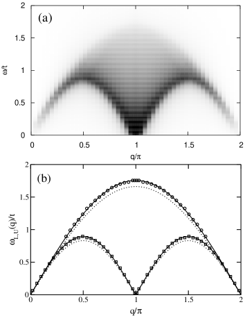
Figure 2: (a) Density plot of the data in Fig. 1. (b) Upper (circles) and lower (squares) onset of the two-spinon continuum extracted from the DDMRG data. Solid lines are fits to the dCP dispersion relations. The dotted line is the dCP dispersion using the exchange coupling $J_{\rm Exp}=0.226$ eV from neutron scattering experiments in SrCuO₂. zaliznyak

The similarity of $S_{\rm MA}(q,\omega)$ with $S(q,\omega)$ in the extended Hubbard model can be seen more clearly in a density plot. Figure 2(a) shows a density plot of the spectral weight distribution. Most spectral weight is located at the lower onset of the two-spinon continuum as in the Heisenberg model. Figure 2(b) shows the lower and upper boundaries of the two-spinon continuum extracted from the DDMRG data. The upper boundary was obtained by analyzing the second derivative ${\mathrm{d}}^{2}S(q,\omega)/{\mathrm{d}}\omega^{2}$ and the lower onset was identified with the position of the low-energy peak. These boundaries are very similar to the dCP–dispersion relations (8a) and (8b) of the Heisenberg model. Fitting our numerical data to these relations we obtain effective exchange couplings $J=0.242{\rm eV}$ (lower boundary) and $J=0.248{\rm eV}$ (upper boundary), respectively (using $t=0.435$ eV). These values are in good agreement with the value $J=0.24{\rm eV}$ reported in our previous work rixs and with the coupling $J_{\rm Exp}=0.226{\rm eV}$ determined from inelastic neutron scattering data for SrCuO₂. zaliznyak As the Müller-Ansatz (7) with the exchange coupling $J_{\rm Exp}=0.226{\rm eV}$ describes the neutron scattering spectrum of SrCuO₂ very well, zaliznyak we conclude that the experimental spectrum is also well described by the spin structure factor of the extended Hubbard model for $U=7.8t,V=1.3t$ and $t=0.435$ eV.

A recent study grage of the spin structure factor in the Hubbard model has shown that there are significant itinerancy effects [a transfer of spectral weight in $S(q,\omega)$ due to the coupling of the spin excitations to charge fluctuations] at low and intermediate values of the Hubbard interaction $U$. In this regime the spin structure factor of the Hubbard model differs from the spectrum $S_{\rm MA}(q,\omega)$ of the Heisenberg model (i.e., the strong-coupling limit $U\gg t$ of the Hubbard model), where charge fluctuations are suppressed and electrons are completely localized. To illustrate this effect we show DDMRG spectra obtained for various parameters $U$ and $V$ on 60-site lattices in Fig. 3. We have normalized $S(q\approx\pi,\omega)$ by the total spectral weight $S(\pi)=\int S(\pi,\omega){\rm d}\omega$, which we obtain by calculating the ground state expectation value $S(\pi)=\langle\psi_{0}\rvert S_{q=\pi}^{z}S_{q=\pi}^{z}|\psi_{0}\rangle$. In these figures the energies are given in units of the two-spinon band width $2W_{s}$, which is equal to $\pi J$ in the Heisenberg model. For $V/t=0$ the value of $W_{\rm s}$ is known exactly from the thermodynamic Bethe-Ansatz solution. theBook When $V/t\neq 0$ we determine $W_{\rm s}$ from the upper onset of the dynamical spin structure factor.

Figure 3: Dependence of the spin structure factor at momentum $q\approx\pi$ on $U$ and $V$. The broadening is $\eta=W_{s}/20$ in the left panel and $\eta=W_{s}/10$ in the other two panels.

Figure 3(a) shows $S(\pi,\omega)$ calculated with a broadening $\eta=W_{s}/20$ for $V/t=0$ and three values of $U/t=0,1,3$. At $U/t=0$ we recover the case of free electrons and accordingly most spectral weight is found in the peak at the upper onset ($\omega=2W_{s}$) of $S(q,\omega)$. When $U/t$ becomes larger the spectral weight is quickly redistributed towards the lower onset at $\omega=0$. Already at $U/t=3$ the upper peak is no longer visible and most spectral weight is found at the lower onset. This supports the analysis of Ref. grage, but shows that itinerancy effects become rapidly weaker for increasing $U$. We now set $V/t=1.3$ and vary $U/t$. The resulting curves $S(\pi,\omega)$ are shown in Figure 3(b). At $U/t=3$ the largest part of the spectral weight is at the low-energy onset. With increasing $U/t$ the low-energy peak becomes more and more pronounced until only little spectral weight remains at the upper onset. For larger interaction strengths the change of the next-nearest neighbor interaction has a weaker influence on the spectral distribution. Figure 3(c) shows $S(\pi,\omega)$ for constant $U/t=7.8$ and varying $V/t$. While the weight of the peak at $\omega=0$ is clearly diminished with growing $V$, the effect appears to be less pronounced than in the case of smaller $U$. In summary, our DDMRG results for the extended Hubbard model confirms that itinerancy effects are important in the dynamical spin structure factor of Mott insulators. grage We note, however, that despite the coupling between spin and charge sectors the upper and lower onsets of the two-spinon continuum are very well described by the dCP relations (8b) and (8a) of the Heisenberg model from strong to intermediate interaction as illustrated by the results in Fig. 2.

Figure 4: Spin structure factor $S(q,\omega)$ at high energies for (a) $U/t=7.8$, $V/t=0$ and (b) $U/t=7.8$, $V/t=3$. The broadening is $\eta=0.2t$. Vertical lines indicate the one-particle gaps $\Delta_{c}$.

Our numerically results reveals another effect of charge fluctuations. The total spectral weight of the spin structure factor is not exhausted by low-energy excitations $\omega(q)\leq\omega_{\text{U}}(q)$. There are dispersive features in that spectrum at energies above the one-particle gap, $\Delta_{c}=E_{0}(1)-E_{0}(1)+2E_{0}(0)$, where $E_{0}(x)$ denotes the ground state energy of the Hamiltonian (II) with $x$ electrons added to or removed from the half-filled system. Figure 4 shows the high energy spectrum of $S(q,\omega)$ for $U/t=7.8$, $V/t=0$ and $U/t=7.8$, $V/t=3$ on a logarithmic scale ($L=60$ in both cases). For energies higher than the one-particle gap we can see that there are dispersive structures up to an energy of roughly twice the one-particle gap. The presence of these spectral features further shows that the coupling to the charge sector affects the spin dynamics of the system.

IV Dynamical Charge Structure Factor

In this section we present numerical results for the dynamical charge structure factor $N(q,\omega)$ of the extended Hubbard model. This correlation function is probed by electron-electron energy loss spectroscopy (EELS). It is also believed to describe the dispersion of peaks and onsets in RIXS experiments rixs .

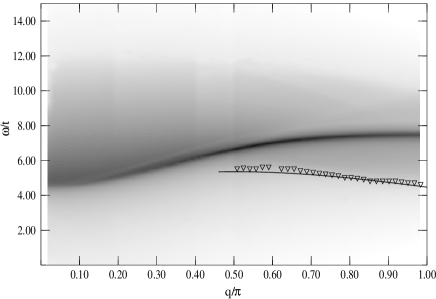
Figure 5: Density plot of the renormalized charge structure factor $N(q,\omega)/q^{2}$ for $U/t=7.8$, $V/t=1.3$. For $q\gtrsim\pi/2$ a solid line follows the spinon dispersion (shifted by the value of the charge gap) and triangles indicate the position of the spectrum onset in the numerical data.

In Fig. 5 we show a density plot of $N(q,\omega)/q^{2}$ for the parameters $U/t=7.8$, $V/t=1.3$ relevant for SrCuO₂. The present DDMRG data are significantly better resolved than in our previous work rixs . Since $\mathrm{lim}_{q\to 0}\int\mathrm{d}\omega\,N(q,\omega)\propto q^{2}$ we have plotted $N(q,\omega)/q^{2}$ on a logarithmic scale in Fig. 5. The momentum resolution is $\Delta q/\pi=1/61$ and the energy resolution is $\eta/t=0.1$ for a system of $L=60$ sites. The most prominent feature is a resonance that disperses downward monotonically starting at the Brillouin zone boundary $q=\pi$. In the strong-coupling limit pencdensity the exciton lies below the continuum for all momenta. Here, in contrast, there is also a substantial spectral weight below the resonance, which clearly lies above the low-energy onset of the continuum shown by triangles for $q\geq\pi/2$ in Fig. 5. As already found in Ref. rixs, this low-energy onset of the continuum follows the spinon dispersion (shifted by the value of the charge gap), which is indicated by a line for $q\gtrsim\pi/2$ in Fig. 5.

The presence of spectral weight below the resonance is particularily blatant at the Brillouin zone boundary. This can be seen clearly in Fig. 6, where we show spectra $N(q\approx\pi,\omega)$ calculated for 60 and 120 lattice sites and the same broadening $\eta/t=0.1$. Both spectra are almost indistinguishable which excludes the possibility that the observed spectral weight is a finite-size effect. In the inset of Fig. 6 the same data are shown on a logarithmic scale. We note that more spectral weight lies below the resonance than above it. Just above the resonance there is a small dip in $N(q\approx\pi,\omega)$ reminiscent of an asymmetric Fano line shapes. fano

Figure 6: Charge structure factor at $q=\pi$ for $U/t=7.8$ and $V/t=1.3$ calculated with a broadening $\eta/t=0.1$. System lengths are $L=60$ (full line) and $L=120$ (open circles). The inset shows the same data on a logarithmic scale.

In our previous work rixs we reported that the extended Hubbard model with $U/t=7.8$, $V/t=1.3$ and $t=0.435$ eV gives an accurate description of the low-energy optical conductivity $\sigma(\omega)=\omega\mathrm{lim}_{q\to 0}N(q,\omega)/q^{2}$ of SrCuO₂. Furthermore, we showed that the low-enery onset and peak dispersions in $N(q,\omega)$ are in quantitative agreement with similar dispersive structures observed in a RIXS experiment. We can also compare our DDMRG results for $N(q,\omega)$ in the extended Hubbard model to the EELS spectrum of Sr₂CuO₃. eels As the model parameters for this material are close to those for SrCuO₂ (see below), we expect to observe the same qualitative features in both cases. Actually, we find that our results for the charge structure factor are in qualitative agreement with the EELS spectrum of Sr₂CuO₃. In particular, the low-energy tail of $N(q,\omega)$ explains the signal observed experimentally below the resonance close to the zone boundary, moskvin a feature which could not be explained by the strong-coupling theory.

To understand the nature of the resonance observed in $N(q\approx\pi,\omega)$ we have performed a finite-size analysis of the peak height $h(\eta(L))$ for different interaction strengths. The broadening is size-dependent such that $\eta L=12t$. ddmrg In strong-coupling theory pencdensity the dispersive resonance is a $\delta$-peak indicating the presence of an exciton. As discussed in Ref. ddmrg, the peak height should diverge as $h(\eta)\propto\eta^{-1}$ in that case. Figure 7 shows a plot of $h(\eta)$ on a double logarithnic scale for various couplings. Clearly, $h(\eta)$ diverges as power law $\eta^{\alpha}$ for $\eta\rightarrow 0$. We extract the exponents $\alpha$ using a linear fit of the logarithms of $h(\eta)$ and $\eta$. The error in the value of the exponent $\alpha$ is 0.01 or smaller. For $U/t\leq 10$ we clearly find that $0>\alpha>-1$, which indicates a power-law divergence in the spectrum $N(q,\omega)$ but no $\delta$-peak. ddmrg In fact, the prediction of the strong-coupling expansion, $\alpha\approx-1$, is only reached (within the numerical accuracy) for extremely large $U/t\geq 100$ (not shown in Fig. 7). This is a first indication that strong-coupling theory becomes accurate only for unphysically large on-site Coulomb interaction.

Figure 7: Scaling analysis of the logarithm of the peak height $h$ in $N(q\approx\pi,\omega)$ as a function of the logarithm of the size-dependent broadening $\eta(L)=12t/L$ for various interaction strengths. Lines are linear fits.

Since the onset of $N(q,\omega)$ follows the spinon dispersion, it is clear that the excited states contributing to the charge structure factor consist in charge excitations hybridized with spin excitations. This is the reciprocal effect of the itinerancy effect in the spin structure factor. The Fano-type line shape of the resonance suggests that it originates from a discrete charge excitation coupled to a continuum of spin excitations. In the strong-coupling limit this discrete charge excitation is an exciton (a neutral bound state of a holon and an anti-holon). As the spin excitation band width goes to zero in that limit, only elastic scattering is possible and thus the exciton has an infinite lifetime and appears as a $\delta$-peak in the spectrum $N(q,\omega)$. For a finite interaction strength, however, spin excitations have a finite band width. Thus neutral bound states have a decay channel into independent charge excitations due to the (inelastic) scattering by spin excitations and therefore their lifetime is finite. Accordingly, the resonance is no longer a $\delta$-peak but a power-law divergence. In particular, for the couplings $U$ and $V$ relevant for real materials, such as the Mott-insulating chain cuprates SrCuO₂ and Sr₂CuO₃, the resonance is not an exciton but corresponds to neutral bound states with a finite lifetime.

As a further check of the strong-coupling theory we directly compare its predictions with our DDMRG results in Fig. 8. The DDMRG data were obtained for a $30$-site lattice and a quite large broadening $\eta/t=0.4$, which smears out fine details. We have convolved the strong-coupling structure factor with a Lorentzian of the same width $\eta$ to enable a direct comparison.

Figure 8: Comparison between the strong-coupling pencdensity (solid lines) and DDMRG (dashed lines) results for the charge structure factor for two sets of model parameters. A broadening $\eta/t=0.4$ is used for both approaches. The momentum varies from $q=0.03\pi$ (top) to $q=0.97\pi$ (bottom).

In Fig. 8(a) we show $N(q,\omega)$ for $U/t=7.64$, $V/t=2.36$. These parameters were chosen in Ref. eels, to explain EELS data of Sr₂CuO₃ using the strong-coupling approach. However, the comparison in Fig. 8(a) reveals large deviations between DDMRG and strong-coupling results for these parameters. Therefore, our results demonstrate that a strong-coupling approach is not accurate in this parameter regime and the parameters $U/t=7.64$, $V/t=2.36$ determined using this approach are not reliable. For comparison, a fit of the experimental optical conductivity and exchange coupling to DDMRG results for the extended Hubbard model (as done in Ref. rixs, for SrCuO₂) yields the parameters $U/t=7.4$, $V/t=1.8$, and $t=0.42$ eV for Sr₂CuO₃. We note that the apparently small difference between strong-coupling and DDMRG parameters has actually radical effects, as the optical absorption spectrum contains an exciton below the Mott gap for $V>2t$ but not for $V\leq 2t$. (Unfortunately, due to the finite experimental resolution it is not clear whether there is such an exciton in the linear optical absorption of Sr₂CuO₃.)

As expected the agreement between strong-coupling theory and DDMRG becomes better for stronger interactions. This can be seen in Fig. 8(b), where we compare $N(q,\omega)$ for $U/t=20$ and $V/t=1$. Nevertheless, in spite of the interaction equaling five times the bare band width $4t$, we still observe significant deviations from the strong-coupling predictions. Similar discrepancies were found previously at coupling as large as $U=40t$ in a study of the optical conductivity, eric-mott which is related to $N(q,\omega)$ through $\sigma(\omega)/\omega=\mathrm{lim}_{q\to 0}N(q,\omega)/q^{2}$.

Figure 9: Charge structure factor $N(q\approx\pi,\omega)$ for $U/t=7.8$ and $V/t=0$ (full line), $V/t=1.3$ (dotted line), $V/t=2$ (short dashed line), $V/t=2.75$ (long dashed line), and $V/t=3.5$ (dashed dotted line). A broadening $\eta=0.1t$ is used.

It has been shown in Ref. eric-optics-ehm, that there are four different types of optical excitations that contribute to $\sigma(\omega)$ depending on the strength of the next-neighbor repulsion $V$. We now study the evolution of $N(q=\pi,\omega)$ with $V$ and discuss how the nature of these excitations influences the dynamical charge structure factor. Figure 9 shows $N(\pi,\omega)$ for $U/t=7.8$ and several values of $V/t$. As expected, we find a broad peak when there is no next-neighbor interaction since the charge excitations do not form long-lived bound states. For $V/t=1.3$ we find a sharp peak with a small but finite intrinsic width. When $V/t=2$ the resonance is weaker and spectral weight leaks to lower energies which leads to a pronounced asymmetry of the peak. This trend continues until the peak is no longer visible in the continuum. The spectral weight is now distributed in a broad band as seen for $V/t=2.75$ in Fig. 9. In the optical conductivity CDW droplets are known to give rise to such a band. eric-optics-ehm Therefore we suggest that the band observed at $q=\pi$ is also related to CDW droplets. When $V$ is further increased a peak appears at low energies which contains most spectral weight. Approaching the CDW phase boundary ($V_{c}/t\approx 3.5$ for $U/t=7.8$) the total spectral weight in that peak $N(\pi)=\int\,{\rm d}\omega N(\pi,\omega)$ (i.e, the static charge structure factor at $q=\pi$) becomes extremely large, which signals the occurrence of the long-range CDW order for $V>V_{c}$.

V One-Particle Spectral Function

We now consider the one-particle spectral function $A(q,\omega)$ of the Hamiltonian (II). This dynamical correlation function corresponds to the spectrum measured in ARPES experiments. A density plot of the spectral function is shown in Fig. 10 for the parameters appropriate for SrCuO₂, $U/t=7.8$ and $V/t=1.3$. These data have been calculated on a 90-site lattice using a broadening $\eta=0.1t$, which yields a momentum resolution $\Delta q=\pi/91$ and an energy resolution of the order of $\eta$. With this resolution spin-charge separation is clearly seen in Fig. 10. The spinon branch is denoted by (S) and has a width $W_{s}=\pi J/2\approx 0.9t\approx 0.4$ eV. The holon branch is labeled (H) and has a width of about $2.7t\approx 1.2$ eV (from $q=0$ to $q=\pi/2$). This spin-charge separation has been observed experimentally in the ARPES spectrum of SrCuO₂. kim ; koi06 The spinon and holon band widths calculated here for $U/t=7.8$ and $V/t=1.3$ are compatible with the experimental data: The latest measurements koi06 yield $0.49\pm 0.13$ eV and $1.42\pm 0.08$ eV, respectively. [Note that the effective hopping term $t$ defined in Ref. koi06, is not equivalent to the bare hopping term $t$ of our model (II).] A further verification of the theoretical description of SrCuO₂ by the extended Hubbard model would be a direct comparison of the experimental spectral weight distribution with our DDMRG data. Unfortunately, the limited resolution of ARPES data and a strong background signal prevent a meaningful comparison.

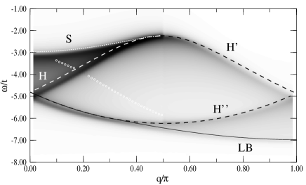
Figure 10: Density plot of the one-particle spectral function $A(q,\omega)$ calculated with DDMRG for $U/t=7.8$ and $V/t=1.3$. The dispersions of elementary excitations in the one-dimensional Hubbard model with $U/t=7.74$ are also shown: Spinon branch (S), holon branches (H,H’,H”) and lower boundary of the holon-spinon continuum (LB). Open white circles mark the position of a step-like feature in the DDMRG spectrum.

In addition to the holon and spinon branches one sees several dispersive structures in the spectral function of the extended Hubbard model, which are quite similar to those found in the Hubbard model ($V=0$). penc-spectral ; senechal ; matsueda To identify these structures we have calculated the exact dispersions of various excitations in a periodic 90-site Hubbard chain using the Bethe Ansatz. The parameter $U/t=7.74$ has been chosen to reproduce the one-particle gap of the extended Hubbard model with $U/t=7.8$ and $V/t=1.3$. The dispersions of the Hubbard model corresponding to the most important features in the spectral function of the extended Hubbard model are shown as lines in Fig. 10. There are the spinon branch (S), the holon branch (H), a secondary holon branch (H’), the continuation of the holon branch (H”), and the lower boundary (LB) of the continuum of excitations consisting of a single spinon and a single holon . In the entire Brillouin zone these dispersions of the Hubbard model follow closely the dispersive structures of the extended Hubbard model. The deviations can be mainly attributed to a change of the spinon and holon band widths. Thus we conclude that in the Mott-insulating regime the spectral functions of the extended Hubbard model are qualitatively similar to those of the Hubbard model.

There is a very weak dispersive structure in $A(q,\omega)$ of the extended Hubbard model which is not visible in the density plot and is indicated by open circles in Fig. 10. This feature is not present in the spectral function of the Hubbard model with $U/t=7.74$. In the extended Hubbard model it consists of a shoulder in the spectrum and can be localized by calculating the first derivative of $A(q,\omega)$. Its dispersion closely resembles the holon dispersion shifted by an offset equal to the spinon band width. However, we do not find this shoulder if we use periodic boundary conditions. Therefore, this feature is a boundary effect due to the abrupt cutting-off of the nearest-neighbor interaction terms at both chain ends.

We note that the spectral function $A(q,\omega)$ of the extended Hubbard model has been investigated previously using a variational CPT approach potthoff for a set of parameters ($U/t=8,V/t=2$) close the one used in Fig. 10. Qualitatively, both spectral functions are very similar and resemble the spectral function of the Hubbard model. penc-spectral ; senechal ; matsueda However, our DDMRG spectra are free of the striped structures which are present in the variational CPT spectral functions. Therefore, we conclude that these striped structures are artifact of the variational CPT approach.

Figure 11: One-particle spectral function $A(q,\omega)$ for various momenta $q$ and three different interaction strengths: $U/t=7.8$, $V/t=1.3$ (dotted line), $U/t=7.8,V/t=3$ (dashed line) and $U/t=7.74$, $V/t=0$ (full line). The broadening is $\eta/t=0.1$.

We now discuss the impact of varying the model parameters on the spectral function $A(q,\omega)$. A comparison of the line shapes is shown in Fig. 11 for various momenta $q$ and three different parameter sets ($U/t=7.8$, $V/t=1.3$), ($U/t=7.8,V/t=3$) and ($U/t=7.74$, $V/t=0$). These data have been calculated for a broadening $\eta/t=0.1$ on a 90-site chain. For $|q|<q_{\text{F}}=\pi/2$ there are only small differences between the line shapes for $V/t=0$ and $V/t=1.3$. The holon and spinon peaks shift according to the change of the holon and spinon band widths. This is clearly visible in the two upper panels of Fig. 11, where spinon and holon peaks are well separated. For a stronger coupling $V/t=3$ a significant transfer of spectral weight occurs from the spinon peak to the holon peak. The low-energy continuation of the holon branch (H”) is also visible as a small third peak in the right upper panel. The two middle panels of Fig. 11 shows the spectral function as $q$ approaches $\pi/2$ from below. There, spinon and holon structures appear to be merged in a single strong peak because the energy difference between spinon and holon is small compared to the broadening $\eta/t=0.1$ used. In these panels one again sees the peak associated with the continuation of the holon branch (H”) at high binding energies ($\omega/t\approx-6$). The spectral weight of this structure diminishes as $V$ increases and this structure is no longer visible for $V/t\geq 3$.

For momenta $|q|>\pi/2$ the total spectral weight is much smaller than for $|q|<\pi/2$, as expected, and diminishes for increasing $V$. Nevertheless we observe several spectral features in the two lowest panels of Fig. 11 which are usually referred to as shadow bands. haas Shifts of the peak position for varying $U$ and $V$ are again related to the change of the spinon- and holon band widths. The distribution of spectral weight is more strongly affected by the value of the nearest-neighbor interaction for $|q|>\pi/2$ than for small momenta $q$. The peaks associated with the shadow band and the secondary holon are well separated in the left panel ($q<\pi$) but have merged in the right panel ($q\rightarrow\pi$). Furthermore, a low energy structure corresponding to the lower boundary of the holon-spinon continuum is also visible around $\omega/t=-7$.

Finally, we have found that there is a little spectral weight below the lower boundary of the holon-spinon continuum. This is most clearly seen in the lowest left panel of Fig. 11 for $V/t=3$. Therefore, excitations made of one holon and one spinon are not sufficient to explain all features of the one-particle spectral function of the extended Hubbard model. Overall, the influence of the nearest-neighbor interaction $V$ on the spectral function is noticeable but not as dramatic as its impact on the spin and charge structure factors. The main features (spinon, holon and shadow bands) are always present with similar dispersions albeit with different spectral weights and band widths as already found with the variational CPT method. potthoff .

VI Summary

We have calculated the dynamical spin and charge structure factors and one-particle spectral function of the one-dimensional extended Hubbard model with on-site ($U$) and nearest-neighbor ($V$) interactions using the dynamical density-matrix renormalization group method. We have investigated how these dynamical correlation functions are affected by variations of the model parameters and discussed the spin and charge dynamics of this model in the Mott insulating regime. For the spin structure factor the strong-coupling picture of the Heisenberg model remains qualitatively valid down to intermediate on-site repulsion $U\sim 4t$, in particular for the parameters relevant for cuprate compounds. Itinerancy effects due to the coupling with charge fluctuations become significant for weak interactions $U\lesssim 3t$. The nearest-neighbor interaction $V$ does not affect the spin structure factor qualitatively. For the charge structure factor, however, the strong-coupling approach fails but for extremely strong interaction $U\gg t$ because the coupling to spin fluctuations becomes relevant as soon as $t/U$ is finite. In particular, it leads to incorrect predictions for the charge dynamics for the parameters appropriate for cuprate compounds. Varying the nearest-neighbor interaction $V$ causes dramatic alterations in the charge structure factor, which reflect changes in the nature of the charge excitations, such as the formation of (quasi-)excitons and CDW droplets. The one-particle spectral function does not change qualitatively with varying parameters within the Mott insulating regime.

Finally, we have shown that the extended Hubbard model allows for a quantitative description of various experiments in the cuprate chains SrCuO₂ and Sr₂CuO₃ with only a single choice of parameters for each material. For SrCuO₂ the extended Hubbard model with $U/t=7.8$, $V/t=1.3$ and $t=0.435$ eV describes the low-energy optical conductivity, the main dispersive features in the RIXS spectrum, and the inelastic neutron scattering spectrum quantitatively. In addition, the one-particle spectral function agrees at least qualitatively with the experimental ARPES spectrum. For $U/t=7.4$, $V/t=1.8$, and $t=0.42$ eV the extended Hubbard model fits the low-energy optical conductivity spectrum and the exchange coupling of Sr₂CuO₃ very well. Moreover, it reproduces the main features of the EELS spectrum of that material at least qualitatively. In conclusion, the extended Hubbard model yields a coherent quantitative description of low-energy electronic excitations in cuprate compounds and thus provides a theoretical framework for studying the spin and charge dynamics of these systems.

We are grateful to F.H.L. Eßler, H. Frahm, F. Gebhard and R.M. Noack for helpful discussions. This work was supported by the Deutsche Forschungsgemeinschaft under Grant No NO 314/1-1. H.B. acknowledges support by the Optodynamics Center of the Philipps-Universität Marburg. Some calculations were performed using Kazushige Goto’s BLAS library.

References

- (1) Strong Interactions in Low Dimensions, edited by D. Baeriswyl and L. Degiorgi (Kluwer, 2004).
- (2) C. Kim, A. Y. Matsuura, Z. –X. Shen, N. Motoyama, H. Eisaki, S. Uchida, T. Tohyama, and S. Maekawa, Phys. Rev. Lett. 77, 4054 (1996); C. Kim, Z. -X. Shen, N. Motoyama, H. Eisaki, S. Uchida, T. Tohyama, and S. Maekawa, Phys. Rev. B 56, 15589 (1997).
- (3) A. Koitzsch, S.V. Borisenko, J. Geck, V.B. Zabolotnyy, M. Knupfer, J. Fink, P. Ribeiro, B. Büchner, and R. Follath, Phys. Rev. B 73, 201101(R) (2006).
- (4) J. Voit, Rep. Prog. Phys. 58, 977 (1995).
- (5) D. Controzzi and F. H. L. Essler, Phys. Rev. B 66, 165112 (2002).
- (6) M.J. Bhaseen, F. H. L. Essler, and A. Grage, Phys. Rev. B 71, 020405 (2005).
- (7) J. Favand, S. Haas, K. Penc, F. Mila, and E. Dagotto, Phys. Rev. B 55, R4859 (1997).
- (8) W. Stephan and K. Penc, Phys. Rev. B 54, R17269 (1996).
- (9) M. Arikawa, Y. Saiga, and Y. Kuramoto, Phys. Rev. Lett. 86, 3096 (2001).
- (10) R. N. Bannister and N. d’Ambrumenil, Phys. Rev. B 61, 4651 (2000).
- (11) D. Senechal, D. Perez, and M. Pioro-Ladrière, Phys. Rev. Lett. 84, 522 (2000).
- (12) M. Aichhorn, H.G. Evertz, W. von der Linden, and M. Potthoff, Phys. Rev. B70, 235107 (2004).
- (13) R. Preuss, A. Muramatsu, W. von der Linden, F. F. Assaad, and W. Hanke, Phys. Rev. Lett. 73, (1994) 732.
- (14) C. Lavalle, M. Arikawa, S. Capponi, F. F. Assaad, and A. Muramatsu, Phys. Rev. Lett. 90, 216401 (2003).
- (15) E. Jeckelmann, Phys. Rev. B 66, 045114 (2002).
- (16) Y.-J. Kim, J. P. Hill, H. Benthien, F. H. L. Essler, E. Jeckelmann, H. S. Choi, T. W. Noh, N. Motoyama, K. M. Kojima, S. Uchida, D. Casa, and T. Gog, Phys. Rev. Lett. 92, 137402 (2004).
- (17) H. Benthien, F. Gebhard, and E. Jeckelmann, Phys. Rev. Lett. 92, 256401 (2004).
- (18) Dynamical Properties of Quasi One-Dimensional Correlated Electron Systems, H. Benthien, PhD. thesis (Marburg, 2005).
- (19) M. Hoinkis, M. Sing, J. Schaefer, M. Klemm, S. Horn, H. Benthien, E. Jeckelmann, T. Saha-Dasgupta, L. Pisani, R. Valenti, and R. Claessen, Phys. Rev. B 72, 125127 (2005).
- (20) H. Matsueda, N. Bulut, T. Tohyama, and S. Maekawa, Phys. Rev. B 72, 075136 (2005).
- (21) I. A. Zaliznyak, H. Woo, T.G. Perring, C.L. Broholm, C.D. Frost, and H.. Takagi, Phys. Rev. Lett. 93, 087202 (2004).
- (22) R. Neudert, M. Knupfer, M.S. Golden, J. Fink, W. Stephan, K. Penc, N. Motoyama, H. Eisaki, and S. Uchida, Phys. Rev. Lett. 81, 657 (1998).
- (23) F.H.L. Essler, H. Frahm, F. Göhmann, A. Klümper, V.E. Korepin, The One–Dimensional Hubbard Model (Cambridge University Press, Cambridge, 2005).
- (24) E. Jeckelmann, Phys. Rev. Lett. 89, 236401 (2002).
- (25) G. Müller, H. Thomas, H. Beck, and J. C. Bonner, Phys. Rev. B 24, 1429 (1981).
- (26) U. Fano, Phys. Rev. 124, 1866 (1961).
- (27) A different explanation has been proposed in A.S. Moskvin, J.Málek, M. Knupfer, R. Neudert, J. Fink, R. Hayn, S.-L. Drechsler, N. Motoyama, H. Eisaki, and S. Uchida, Phys. Rev. Lett. 91, 037001 (2003).
- (28) E. Jeckelmann, F. Gebhard, and F. H. L. Essler, Phys. Rev. Lett. 85, 3910 (2000).
- (29) E. Jeckelmann, Phys. Rev. B 67, 075106 (2003).
- (30) S. Haas and E. Dagotto, Phys. Rev. B52, 14396 (1995).