Also at ]Landau Institute of Theoretical Physics.

Quantum Shock Waves -
the case for non-linear effects in dynamics of electronic liquids

Abstract

Using the Calogero model as an example, we show that the transport in interacting non-dissipative electronic systems is essentially non-linear. Non-linear effects are due to the curvature of the electronic spectrum near the Fermi energy. As is typical for non-linear systems, propagating wave packets are unstable. At finite time shock wave singularities develop, the wave packet collapses, and oscillatory features arise. They evolve into regularly structured localized pulses carrying a fractionally quantized charge - soliton trains. We briefly discuss perspectives of observation of Quantum Shock Waves in edge states of Fractional Quantum Hall Effect and a direct measurement of the fractional charge.

1.

It is commonly assumed that a small and smooth perturbation of electronic systems remains small and smooth in the course of evolution. This assumption justifies the linear response theory to electronic transport. Although it is true for dissipative electronic systems, like a metal, it fails for dissipationless quantum fluids.

In this paper we argue that in such electronic systems, commonly known in one spatial dimension, the transport is essentially non-linear and is subject to an unstable singular behavior. An arbitrarily small and smooth disturbance of electronic density and momentum (a wave packet) will inevitably develop to shot-noise-like oscillatory features, progressively evolving to regular localized pulses, carrying quantized charge - a soliton train. This process is a dissipationless counterpart of a shock wave, where an initially smooth profile of density tends to overhang and collapse at some finite time. A typical behavior is shown in Fig. 1. We will demonstrate this phenomenon on the example of the Calogero model, but believe that a shock wave instability and the main features of the subsequent dynamics are universal for dissipationless interacting electronic systems. They are insensitive to details of interactions and to the initial profile of the wave.

We note that, for some physical systems, the time of the onset of the shock wave may be longer than the time needed for other physical mechanisms to dissipate the disturbance. However, our estimates indicate that the observation of shock waves at confined states of a quantum well heterostructures (the edge states of Fractional Quantum Hall Effect (FQHE) ) is possible. In addition, a dynamic experiment may allow direct observation of the fractional charge of “fly-out” excitations.

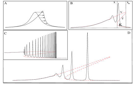
Figure 1: Numerical solution of BO equation (8). A: The initial Lorentzian profile containing 7 solitons is shown at time $t=0.9t_{c}$. B: The wave after a shock is shown together with the overhanging solution of Riemann equation (5) (red, dashed) at $t=2.7t_{c}$. Vertical lines mark the trailing and the leading edges. The moduli $v,\tilde{v},K$ of the 1-phase solution (9) are assigned to different branches of the multi-valued solution of (5). D: The solutions of BO and Riemann’s equations are shown at $t=11t_{c}$. C: Whitham modulated wave represents an approximate soliton train behavior for an initial Lorentzian shape of a larger area.

2. Calogero-Sutherland model

defined on a circle by

$${\cal H}=-\sum_{j=1}^{N}\frac{\hbar^{2}}{2m}\frac{\partial^{2}}{\partial x_{j}^{2}}+\sum_{k\neq j=1}^{N}\frac{\pi^{2}}{2L^{2}}\frac{g}{\sin^{2}(\frac{\pi}{L}(x_{j}-x_{k}))}$$ (1)

occupies a special place in 1D quantum physics. The singular interaction is so strong that it changes the statistics of particles from $1$ (Fermi-statistics) to $\lambda$, while excitations carry statistics of $1/\lambda$ (for a review see e.g., 1999-Polychronakos ; Ha ). The chiral sector of Calogero model, therefore, describes the edge of the FQHE with a fractional filling $1/\lambda$. Here $\lambda$ is a dimensionless coupling constant $g=\frac{\hbar^{2}}{m}\lambda(\lambda-1)$. Below we set $a=(\lambda-1)/\lambda$ , $\kappa=2\pi\lambda\hbar/m$, and rely on results of Abanov and Wiegmann (2005).

3. Evolution of a semiclassical state.

Consider an evolution of an initial state - a wave-packet $|\Psi\rangle$, of a “large” size $l\gg k_{F}^{-1}$ as on Fig. 1A. The state is assumed to be semiclassical, i.e., it involves many particles, and is such that its Wigner’s function $W(x,p)=\langle\Psi|e^{\frac{i}{\hbar}(\hat{P}x+p\hat{X})}|\Psi\rangle$ has a well-defined classical limit. This means that $W(x,p)$ exponentially vanishes outside of a certain star-like support in phase space. Semiclassical hydrodynamic modes can be viewed as area-preserving waves of the boundary of the support. We study the time evolution of the density $\rho(x,t)=\int W(x,p,t)dp$ and current $j(x,t)=\int pW(x,p,t)dp$, or velocity $v(x,t)$ defined as $j=m\rho v$ of the wave-packet. The state can be created by some classical instrument acting on a system.

First, we argue that in interacting 1D system like (1) the evolution of a semiclassical state is determined only by hydrodynamic variables – the density $\rho(x,t)$ and velocity $v(x,t)$. In other words, the semiclassical density and velocity obey a set of closed evolution equations of hydrodynamic type. Things are different for non-interacting particles $\lambda=1$. There, a “gradient catastrophe” also occurs at a finite time, but further evolution has an essentially quantum nature.

4. Quantum hydrodynamics.

To study the dynamics of (1) and similar problems, it is productive to represent a quantum many body problem as quantum hydrodynamics, i.e., rewrite it solely in terms of the density $\rho(x)\!=\!\sum_{i}\delta(x-x_{i})$ and the velocity operators $\left[\rho(x),v(y)\right]\!=\!-\!i\frac{\hbar}{m}\delta^{\prime}(x-y)$ f . In this approach Sakita-book excitations appear as solitons of nonlinear fields $\rho(x)$ and $v(x)$. Calogero model has been successfully written in terms of hydrodynamic variables, thus extending the familiar “bosonization” of fermionic models in 1D Jevicki-1992 ; Awata ; AJL-1983 ; Abanov and Wiegmann (2005). Below we remind the major facts following Abanov and Wiegmann (2005).

Equations of motion of (1) are equivalent to equations of quantum hydrodynamics

$${\rm continuity\,equation}: \qquad\dot{\rho}+\nabla(\rho v) =0,$$ (2)

$${\rm Euler\,equation}: \qquad\dot{v}+\nabla(\frac{v^{2}}{2}+w) =0,$$ (3)

where $\quad w=(\kappa/2\pi)^{2}\delta(\rho\epsilon)/\delta\rho$ is the quantum enthalpy and $\epsilon$ is the energy per particle in units of $\lambda\kappa/2\pi$

$$\epsilon=\frac{1}{6}(\pi\rho)^{2}+\frac{a^{2}}{8}(\nabla\ln\rho)^{2}+\frac{1}{2}\pi a\nabla\rho_{H},$$ (4)

and $\rho_{H}=\mathop{\text{\makebox[0.0pt][l]{\makebox[4.16669pt]{$-$}}$\int_{0}^{L}$}}\frac{dx^{\prime}}{L}\rho(x^{\prime})\cot\frac{\pi}{L}(x^{\prime}-x)$ is a Hilbert transform of the density. The first term in (4) is present already for free Fermi gas ($\lambda=1$) - the Fermi energy. The last two terms absent at $\lambda=1$ reflect the interaction.

5. Sound waves, nonlinear effects and dispersion.

In the limit of small deviations of density $\delta\rho\!=\!\rho\!-\!\rho_{0}\!\ll\!{\rho_{0}}$, and velocity $\delta v\!=\!v\!-\!v_{0}\!\ll\!v_{0}$ from their mean values $\rho_{0}$ and $v_{0}$, eqs. (2,3) may be linearized. If in addition gradients are small $a\frac{\nabla\delta\rho}{\delta\rho}\ll\rho_{0}$ so that the two last terms in (4) can be dropped, one obtains the familiar “linear bosonization”, where density and velocity waves move to the right (left) with Fermi velocities $v_{F}=v_{0}\pm\frac{\kappa}{2}\rho_{0}$ without dispersion. Introducing left and right moving fields $u=\delta v\pm\frac{\kappa}{2}\delta\rho$ the linear hydrodynamics reads $\dot{u}+v_{s}\nabla u=0$, where $v_{s}=v_{F}$ are velocities of sound.

Shifting to a Galilean frame moving with velocity $v_{s}$, one recovers non-linear effects:

$$\dot{u}+u\nabla u=0.$$ (5)

This is is the quantum Riemann equation for 1D compressible hydrodynamics Landau_book . Its follows from the Galilean invariance and may be traced to a curvature of the particle spectrum. The Riemann equation states that the wave $u(x,t)$ moves with a velocity which is itself given by $u(x,t)$. Contrary to the case of a linear spectrum, when a packet moves with the velocity of sound, and does not change its shape, an arbitrarily small dispersion deforms the packet pushing its denser part forward.

Eq. (5) is equivalent to (2,3) under assumption of small gradients $a\nabla\delta\rho\ll\delta\rho^{2}$ when the two last terms in (4) are small. However this assumption almost never holds. It fails for any small and smooth initial condition with a “bright side” when $u(x)\nabla u(x)<0$ (Fig. 1A). This is seen from the implicit solution of (5) due to Riemann: $u=f(x-u\,t)$, where $f(x)=u(x,0)$ is the initial state. The bright side of the wave packet steepens and finally overturns at some time, $t_{c}$, where the formal solution becomes multi-valued Landau_book , and un-physical Fig. 1B-D.

Hydrodynamics of the electronic system can be understood as a hydrodynamics of the Fermi sea drawn in the phase space (or more precisely of the support of the Wigner’s function in the phase space). In equilibrium it is bounded by two lines $k_{F}^{(\pm)}=m(v_{0}\pm\frac{\kappa}{2}\rho_{0})$. The field $mu(x,t)$ is interpreted as a wave propagating on the Fermi surface in the phase space.

The time $t_{c}$ is roughly the time for the top of the wave-packet to travel a distance of its size $l$. Since the excess velocity is $u$, an overhang occurs at a time $t_{c}\!\sim\!l/(\delta v\pm\frac{\kappa}{2}\delta\rho)$. At this time a curvature of the spectrum becomes a dominant factor. Obviously, a smooth and small packet remains in the linear regime longer, but its life is finite. In the vicinity of the overhang the classical Riemann equation becomes invalid. A shock must be regularized either by quantum corrections at $\lambda=1$, or, in the interacting case, by the neglected gradient terms.

6. Dispersive regularization - the role of interaction.

The role of dispersion changes in the presence of an interaction. The latter gives higher gradient corrections to the Euler equation. In the linear regime they are small, but in the shock-wave regime, they stabilize growing gradients. This mechanism is called dispersive regularization, and is well known in the theory of non-linear waves book . A stabilization occurs when dispersive and nonlinear terms in (4) become of same order

$$a\nabla\delta\rho\sim\delta\rho^{2}.$$ (6)

This condition determines the smallest scale of oscillations occurring after a shock wave. It is $\Delta l\sim a/\delta\rho$.

This is an important result. Rising gradients are bounded by a scale exceeding the Fermi length $k_{F}\Delta l\!\gg\!1$.

As a consequence a semiclassical wave packet of interacting 1D-fermions remains semiclassical even after entering a shock wave regime. Its evolution is described by a classical non-linear hydrodynamics.

Condition (6) emphasizes the role of interaction. In its absence ($\lambda=1$) the gradient catastrophe is stabilized only by quantum effects and makes a semiclassical description non-valid at $t\sim t_{c}$ .

7. Chiral case

A generic wave-packet will be separated into two parts - left and right modes moving away with sound velocities. The physics of shock waves is featured in each chiral part, so we can treat them separately. Moreover, specifics of the Calogero model allows us to separate the chiral sectors exactly, by choosing initial conditions as ${\rm v}=\frac{\kappa}{2}\rho,$ so that the motion is only (right) chiral. Here ${\rm v}\!=\!v\!-\!a\frac{\kappa}{4\pi}\nabla(\log\rho)_{H}$ is the shifted velocity Hermitian with respect to the inner product f . Under this condition two eqs. (2,3) become identical

$$\dot{\rho}+\frac{\kappa}{2}\nabla(\rho^{2}+\frac{a}{2\pi}\rho\nabla(\log\rho)_{H})=0.$$ (7)

8. Benjamin-Ono equation.

Equation (7) admits further simplification relevant for the physics of shock waves. The semiclassical nature of the initial wave packet insures that deviations of density from the mean value, $\rho_{0}$ are small. Let us choose the chiral case, and a frame moving with the velocity $v_{s}=\kappa\rho_{0}$. Then keeping gradient terms in (7) of the lowest order, we linearize the dispersion term $\rho\nabla(\log\rho)_{H}\!\approx\!\nabla(\delta\rho)_{H}$. As a result we obtain the celebrated Benjamin-Ono (BO) equation

$$\dot{u}+u\nabla u+a\frac{\kappa}{4\pi}\nabla^{2}u_{H}=0,\quad u=\kappa\delta\rho.$$ (8)

In hydrodynamics it describes interface waves in a deep stratified fluid AC . Eqs. (2,3) having a similar structure but capturing both chiral sectors, were called Benjamin-Ono equation on the double (DBO) in Abanov and Wiegmann (2005). Both eqs. (7,8) are quantum. The field $u$ in the quantum BO eq. is the gradient of a canonical real Bose field.

9. Quantum Benjamin-Ono equation and FQHE.

It is commonly accepted that edge states in FQHE are described by chiral bosons 2003-Chang . The quantum BO equation is a good candidate for an extension of the theory of edge states beyond the linear approximation. Indeed, it has all the necessary features of the physics of edge states: in the linear approximation it reduces to linear chiral bosons, the statistics of excitations is fractional, and it is Galilean invariant. Elsewhere we argue that the Galilean invariance and statistics uniquely determine both the nonlinear and the dispersion terms of the equation.

10. Semiclassical hydrodynamic equations, solitons. Below we study a semiclassical version of quantum hydrodynamics. Due to a non-linear nature of quantum equations, the semiclassical limit is more subtle than merely treating quantum operators as classical fields. In Abanov and Wiegmann (2005) we argued that the semiclassical limit describes a collective motion of excitations (quasi-holes) with charge $1/\lambda$. This amounts to replacing the parameter $a$ in (2,3,7,8) by the charge of excitation ${1}/{\lambda}$ . To see this, one may notice that the parameter $a$ is a charge of solitons of the classical non-linear field $u$.

Solitons and more general multiphase solutions of BO are known 1979-SatsumaIshimori ; Dobrokhotov and Krichever (1991). We have found general multiphase solutions and their Whitham modulations for more general DBO eqs.(2,3). We present these results elsewhere paper5 . Here we restrict ourselves to a simplified description of a shock wave in the most physically relevant limit when BO (8) holds. To this end we need to know only 1-phase and 1-soliton solutions.

The one-phase solution (compare to Polychronakos-1995 ) reads

$$\delta\rho-\overline{\delta\rho}\!=\!\frac{1}{\pi\lambda}{\rm Im}\partial_{x}\log\Big{(}1\!-\!\sqrt{\frac{v\!-\!K}{\tilde{v}\!-\!K}}e^{\frac{i}{\hbar}\theta(x,t))}\Big{)},$$ (9)

where $\theta(x,t)=k(x-Vt)$, $k=m(v-\tilde{v})$, $V=\frac{1}{2}(v+\tilde{v})$ and $\overline{\delta\rho}=\frac{2}{\kappa}(K+\frac{k}{m})$ are the phase, the wave number, the velocity and the mean density. Parameters $v,\tilde{v}$ and $K$ are the moduli of the solution.

The 1-soliton solution appears as a long wave limit $k\!\to\!0$ of (9)

$$\delta\rho-\overline{\delta\rho}=\frac{1}{\pi\lambda}{\rm Im}\frac{1}{x-Vt-i\frac{\hbar}{2m(V-\frac{\kappa}{2}\overline{\delta\rho})}}.$$ (10)

The amplitude, $\frac{4(V-\frac{\kappa}{2}\overline{\delta\rho})}{\kappa}$, and the width, $\frac{\hbar}{2m(V-\frac{\kappa}{2}\overline{\delta\rho})}$ of the soliton are determined by the excess velocity $V-\frac{\kappa}{2}\overline{\delta\rho}$. The charge of the soliton is $1/\lambda$.

11. Whitham modulation.

Although eqs. (2,3,7,8) are integrable, only quasi-periodic solutions enjoy explicit formulas paper5 . Solutions with generic initial data can not be found explicitly. However, in many physically motivated cases, the solutions are well-approximated by slowly modulated waves. There it is assumed that the moduli of a quasi-periodic solution (in the case of 1-phase solution (9) the moduli are $v,\tilde{v},K$) also depend on space and time but in a slow manner. They do not change much during a period of oscillation. If the scales of oscillations and modulations are separated, the Whitham theory provides equations for the space-time dependence of the moduli Whitham .

Shock waves is the most spectacular application of the Whitham theory. It has been developed in a seminal paper GP on the example of the KdV equation. The idea of the method is the following. Outside the shock wave regime a smooth initial wave remains smooth, and one legitimately neglects the dispersion term, keeping only non-linear terms. The equation obtained in this manner is the Riemann eq. (5). Its solution with initial condition $u(x,0)=f(x)$ reads $u^{(0)}(x,t)=f(x-u^{(0)}(x,t)\cdot t)$. By using the superscript we indicate that this is not the oscillatory part of the solution. A solution of (5) always overturns, and, typically becomes a three-valued function in the interval $x_{-}(t)<x<x_{+}(t)$ (Fig.1 B), where the leading and trailing edges $x_{\pm}(t)$ are determined by the condition $\partial_{x}u^{(0)}=\infty$. Let us order the branches as $u^{(0)}_{1}>u^{(0)}_{2}>u^{(0)}_{3}$.

In the three-valued region the dispersion is important. It replaces a non-physical overhang by modulated oscillations. The latter are given by the Whitham’s modulated solution. To leading order one chooses a modulated 1-phase solution. We call it $u^{(1)}(x,t)$ to emphasize that this solution has only one fast harmonic. It is glued with $u^{(0)}$ at $x_{\pm}(t)$: $u^{(0)}_{1}(x_{-})=u^{(1)}(x_{-}),\,u^{(0)}_{3}(x_{+})=u^{(1)}(x_{+})$.

A modulated 1-phase solution is given by the formula (9), where three moduli $v,\,\tilde{v},\,K$ are smooth functions of space-time, and the phase $\theta(x,t)$ is replaced by a modulated phase $\Theta(x,t)$ found from the Whitham equations

$$\nabla\Theta=m(v-\tilde{v}),\quad\dot{\Theta}=\frac{m}{2}(v^{2}-\tilde{v}^{2}).$$

The Whitham equations for the moduli have again the form of Riemann equation (5)

$$\dot{v}+v\nabla v=0,\;\;\;\,\,\,\dot{\tilde{v}}+\tilde{v}\nabla\tilde{v}=0,\;\;\;\,\,\,\dot{K}+K\nabla K=0.$$

The boundary data for the moduli are chosen such that $u^{(1)}$ stops to oscillate at the gluing points $x_{\pm}$. That happens (i) when $v\to\tilde{v}$ at $x=x_{+}(t)$, there $u^{(1)}\to K$, and (ii) when $\tilde{v}\to K$, at $x=x_{-}(t)$, there $u^{(1)}\to\tilde{v}$. The gluing conditions lead to an especially simple result for the moduli of BO equation Dobrokhotov and Krichever (1991); Matsuno (1998):

$$v=u^{(0)}_{1}(x,t),\;\tilde{v}=u^{(0)}_{2}(x,t),\;K=u^{(0)}_{3}(x,t).$$

12. Shock waves.

The space-time dependence of the moduli approximately determines the entire evolution of a wave-packet. We summarize some features which are not sensitive to its initial shape. Let us choose a frame moving with the sound velocity. An initially smooth bump with a height $\delta\rho$ and a width $l$ tends to overhang toward its bright side. Its dark side becomes smoother. At the time $t_{c}\sim l/\kappa\delta\rho$ the bump starts to produce oscillations. The oscillations fill the growing interval $x_{-}(t)\!<\!x\!<\!x_{+}(t)$. Further, at $x>x_{+}(t)$ the shape of the bump does not change.

The leading edge runs with an excess velocity with respect to the sound. At large time $x_{+}\sim\kappa\delta\rho\cdot t$.

The trailing edge $x_{-}$ slows down with time. If initial bump decays as $\delta\rho(x,0)\sim x^{-n}$, then at large time $x_{-}(t)\sim t^{1/(n+1)}$. If the decay is exponential $\delta\rho(x,0)\sim e^{-x/r}$, then $x_{-}(t)\sim r\log t$. These are the simple consequences of the Riemann equation (5).

The amplitude of oscillations is zero at the trailing edge and grows towards the leading edge. Furthermore, the period of the oscillations also grows. As a result, near the leading edge the oscillatory pattern resembles a collection of individual localized traveling pulses (solitons) - a soliton train. The excess velocity, $V-\frac{\kappa}{2}\overline{\delta\rho}$, of the leading soliton is $\kappa\delta\rho$, which also determines the amplitude $4\delta\rho$. The hight of the leading pulse is four times higher than the initial bump. Since each pulse carries a quantized charge $1/\lambda$, the width of leading pulses, $(4\pi\delta\overline{\delta\rho}\lambda)^{-1}$ stays constant, while the distance between them is growing.

15. Observation of shock waves and direct measurement of a fractional charge.

Edge states of FQHE seems to be the best electronic system to observe quantum shock waves. In order to evaluate the scales one needs parameters of the linearized theory of the edge - the sound velocity and the compressibility of the chiral boson. Although these quantities have never been measured directly, one can suggest reasonable estimates Kang . We estimate the sound velocity on the edge as $v_{s}\sim 3\times 10^{4}$m/s. 1998-MG An electronic density in the bulk $10^{11}$cm^-2 gives an estimate for the 1D density on the edge $\rho_{0}\sim 3\times 10^{7}$m^-1. It gives $\kappa=v_{s}/\rho_{0}\sim 10^{-3}$m²/s, and, at $\lambda=3$ estimates an effective mass $m$ to be about 30 electron band masses in GaAs and the “Fermi” time $\tau_{F}=(\kappa\rho_{0}^{2})^{-1}$ to be $\sim 1$ps.

A wave-packet of width $l\!\sim\!10^{2}\rho_{0}^{-1}\!\sim\!1\mu$m and of height $\delta\rho\!\sim\!10^{-\!1}\rho_{0}$ carrying about 10 electrons, develops a shock wave at time $t_{c}\!\sim\!\tau_{F}(\rho_{0}l)\frac{\rho_{0}}{\delta\rho}\!\sim\!1$ns. During the time $t_{c}$ the wave packet crosses a distance $v_{s}t_{c}\!\sim\!30\mu$m. This scale is much smaller than a size of a typical heterostructure ($\!\sim\!10^{3}\mu$m), and is still smaller than the typical ballistic length $50\!-\!100\mu$m. Distinct solitons will start to appear right after the shock. Observation of the electric charge carried by a distinct soliton-pulse will provide a direct measurement of fractional charge. The full decay of this packet is about $10^{3}$ times longer.

These estimates suggest that non-linear effects (shock waves and fractionally charged soliton train) can be observed in the nanosecond range. Finally, we mention that quantum shock-waves in Bose systems have already been observed in trapped alkali atoms atoms .

We have benefited from discussions with O. Agam, I. Krichever, B. Spivak, A. Zabrodin, V. Goldman, and W. Kang. Our special thanks to I. Gruzberg, D. Gutman, R. Teodorescu. P.W. and E.B. were supported by NSF MRSEC DMR-0213745 and NSF DMR-0220198. AGA was supported by NSF DMR-0348358.

ADDENDUM. In this Addendum we provide some details of the quantum Double Benjamin-Ono equation and its classical solution. A fuller account will be published in paper5 .

1. Holomorphic Bose field.

The seemingly complicated equations, (2,3,4), possess integrable structure, following from the integrability of the Calogero model. This structure becomes more transparent in terms a anti-Hermitian f holomorphic Bose field $\varphi(z)$ and its current ${\rm u}=-i\frac{\kappa}{2\pi}\nabla\varphi(z)$ defined in the complex plane $z=e^{i\frac{2\pi}{L}x}$ Abanov and Wiegmann (2005). The Bose field is a Laurent series with respect to the unit circle $\varphi=\varphi_{+}(z)+\varphi_{-}(z)$ having mode expansion outside of the unit circle

$$\varphi_{+}(z)\!=\!\frac{1}{\lambda}\sum_{n>0}\frac{1}{n}{\rm v}_{n}z^{n},\;\;\varphi_{-}\!=\!\sum_{n<0}\frac{1}{n}\rho_{n}z^{n}+\frac{N}{2}\log z,\;\;$$

$$[\rho_{n},{\rm v}_{-m}]=n\delta_{nm}.$$

Corresponding currents are ${\rm u}_{-}=-i\frac{\kappa}{2\pi}\nabla\varphi_{-},\;{\rm u}_{+}=-i\frac{\kappa}{2\pi}\nabla\varphi_{+}$.

The current is defined as a holomorphic operator having boundary values on the circle

$${\rm u}_{+}(x) = v-i\frac{\kappa}{2}\rho_{H}+ia\frac{\kappa}{4\pi}\partial_{x}\log\rho,$$ (11)

$${\rm u}_{-}(x\pm i0) = \frac{\kappa}{2}(i\rho_{H}\mp\rho).$$ (12)

Its jump is the proportional to the density ${\rm u}(x+i0)-{\rm u}(x-i0)=-\kappa\rho(x)$, thus defining the modes of the negative part of the Laurent series through the moments of coordinates $\rho_{n}=\oint e^{-i\frac{2\pi}{L}xn}\rho(x)dx$.

Let ${\rm u}_{+}(z)$ and ${\rm u}_{-}(z)$ be positive and negative parts of the Laurent series for the current. We have ${\rm u}_{-}=\frac{\kappa}{2}\oint\frac{dx}{L}\,\rho(x)\frac{z+e^{i\frac{2\pi}{L}x}}{z-e^{i\frac{2\pi}{L}x}}$ . This field ${\rm u}_{-}(z)$ is analytic inside and outside the unit disk, having a jump on its boundary equal to the density. The fact that the jump is real implies a reflection property

$$(\varphi_{-}(z))^{\dagger}=\varphi_{-}(1/\bar{z}).$$ (13)

The field $u_{+}(z)$ is an analytic field in some strip $R_{1}<|z|<R_{2}$ surrounding the circle, having value $u_{+}(x)=v-i\frac{\kappa}{2}\rho_{H}+ia\frac{\kappa}{4\pi}\partial_{x}\log\rho$ on the circle. Under the chiral condition it becomes $u_{+}(x)=\frac{\kappa}{2}(\rho-i\rho^{H})+ia\frac{\kappa}{4\pi}\nabla(\log\rho-i(\log\rho)^{H})$. In this case $u_{+}(z)$ becomes analytic inside the circle (i.e., $R_{1}=0$ in the chiral case).

2. Quantum bilinear equation

In terms of the Bose field the equations of quantum hydrodynamics are written in a compact wayAbanov and Wiegmann (2005). Let us introduce positive/negative vertex operators $\tau_{+}=e^{-\varphi_{+}}$ and $\tau_{-}=e^{\lambda\varphi_{-}}$. Then eqs. (2,3) are equivalently written in the form of quantum bilinear Hirota equation

$$(iD_{t}-\frac{\hbar}{2m}D_{x}^{2})\,\tau_{-}\cdot\tau_{+}=0$$ (14)

with the reflection condition

$$\quad z^{-\lambda(2N-L\Phi)}(\tau_{-}(1/\bar{z}))^{\dagger}=\tau_{-}(z),$$ (15)

where $\Phi$ is some constant. Hirota’s derivatives are defined as $D_{x}^{n}f\cdot g=(\partial_{x}-\partial_{x^{\prime}})^{n}f(x)g(x^{\prime})|_{x=x^{\prime}}$. The bilinear equation is a bosonized version of Calogero model. Its derivation from the original model and the derivation of the quantum hydrodynamic eqs. (2-4) from the bilinear equation is straightforward, but not effortless. Having a solution of these equations one finds the density and velocity $\rho=\frac{1}{\lambda\pi}\nabla\log\tau_{-}$, $v=\frac{\kappa}{2}\frac{1}{\lambda\pi}{\rm Im}\nabla\log\tau_{+}$. The classical version of (14), not bounded by a reflection condition, is known as MKP (modified Kadomtsev-Petviashvili) equation. Here it appears in a quantum version.

3. Reductions of MKP: Benjamin-Ono and Double Benjamin-Ono equations.

The bilinear form is the most economical way to understand connections between eqs. (2,3,7,8):

• The reflection condition (15) implies a reduction of MKP equation to the Double Benjamin-Ono equation (2,3).

• Further requirement that $\tau_{+}$ is an analytical operator inside the unit disk implies the chiral conditions leading to eq. (7).

• Finally further reduction $u_{-}(z)=\overline{u_{+}(1/\bar{z})}+C$, where $C$ is a real constant, leads to the Benjamin-Ono equation (8) 1979-SatsumaIshimori .

We publish a detailed study of this equation elsewhere paper5 . Here we present the few major facts.

4. Semi-classical limit

The classical limit is straightforward in the bilinear form of the quantum equation. There we simply treat $\tau_{+}$ and $\tau_{-}$ as classical fields satisfying (14) and (15).

Let us set $u_{\pm}=\mp\frac{\hbar}{m}i\partial_{x}\log(\tau_{\pm})$, then the classical bilinear equation (14) reads

$$\dot{u}+u\nabla u+\frac{\hbar}{2m}\nabla^{2}\tilde{u}=0$$

where $u=u_{+}+u_{-}$ and $\tilde{u}=i(u_{-}-u_{+})$.

5 Multiphase solution

A general quasi-periodic (or $N$-multiphase) solution of classical MKP equation (2,3) (in the frame where the center of mass of the system is at rest) is coded by $2N$ parameters - $v_{i},\tilde{v}_{i}$ (wave number $k_{i}=m(v_{i}-\tilde{v}_{i})$ and velocities $V_{i}=\frac{1}{2}(v_{i}+\tilde{v}_{i})+v_{0}$ of waves), $N$ real phases $x_{i}$, $2N$ real positive amplitudes $c_{i}^{\pm}$ and two zero modes $K$ and $v_{0}$. It is given by a determinant formula for the tau-functions

$$\tau_{\pm}(x+i0,t)=e^{\frac{i}{\hbar}\theta_{\pm}}\det_{i,j\leq N}\left(\delta_{ij}-c_{i}^{\pm}\frac{e^{\frac{i}{\hbar}\theta_{i}(x,t)}}{v_{i}-\tilde{v}_{j}}\right).$$ (16)

Here $\theta_{i}(x,t)\!=\!k_{i}(x-x_{i}-V_{i}t)$ and $\theta_{-}=-mK(x-\frac{K}{2}t)$, $\theta_{+}=mv_{0}(x-(\frac{1}{2}v_{0}+K)t)$, where $k_{i}=v_{i}-\tilde{v}_{i}$, and $V_{i}=\frac{\tilde{v}_{i}+v_{i}}{2}+v_{0}$.

The reflection property, (15), further restricts the amplitudes

$$(c_{i}^{(\pm)})^{2}\!=\frac{k_{i}^{2}}{m^{2}}\left(\!\frac{v_{i}\!-\!K}{\tilde{v}_{i}\!-\!K\!}\!\right)^{\pm 1}\!\left(\!\frac{v_{i}+\!K\!-\!\Phi}{\tilde{v}_{i}+\!K\!-\!\Phi}\!\right)\frac{\prod_{j\neq i}(\tilde{v}_{j}\!-\!v_{i})(v_{j}\!-\!\tilde{v}_{i})}{\prod_{j\neq i}(v_{j}\!-\!v_{i})(\tilde{v}_{j}\!-\!\tilde{v}_{i})},$$

where $\Phi=\frac{1}{m}\sum_{i}k_{i}$. The parameter $\Phi$ determines monodromy of the wave function. It is the flux piercing the circle. Additional restrictions on $v_{i},\tilde{v}_{i}$ insure that $c_{i}$ are real. The zero mode $K$ is related to the mean density $\rho_{0}=\frac{2}{\kappa}(\Phi+K)$. The mean velocity is $v_{0}$.

One-phase solution was found in Polychronakos-1995 .

The chiral case occurs when all zeros of $\tau_{-}$ are located outside the unit disk of the complex plane $z=e^{i\frac{2\pi}{L}x}$, while all zeros and those of $\tau_{+}$ are inside the unit disk. Solutions of the BO eq. (8) arise at the limit $\frac{v_{i}-K}{K}\to 0$. This yields (16) with the amplitudes 1979-SatsumaIshimori

$$(c_{i}^{(\pm)})^{2}\!=\frac{k_{i}^{2}}{m^{2}}\left(\!\frac{v_{i}-K}{\tilde{v}_{i}-K}\!\right)^{\pm 1}\frac{\prod_{j\neq i}(\tilde{v}_{j}\!-\!v_{i})(v_{j}\!-\!\tilde{v}_{i})}{\prod_{j\neq i}(v_{j}\!-\!v_{i})(\tilde{v}_{j}\!-\!\tilde{v}_{i})}.$$

6. Multisoliton solutions

of the DBO equations (2,3) appear as a long-wave limit of (16), obtained by taking $k_{i}\to 0$, while keeping $V_{i}$ fixed:

$$\tau_{\pm}\!=\!e^{-\frac{i}{\hbar}\theta_{\pm}}\!\det\left((x\!-\!x_{i}\!-\!V_{i}t\!-\!iA_{i}^{\pm})\delta_{ij}\!-\!\frac{i\hbar}{m}\frac{1\!-\!\delta_{ij}}{V_{i}\!-\!V_{j}}\right),$$

where $A_{i}^{\pm}=\frac{\hbar}{2m}\left(\frac{1}{V_{i}+K}\pm\frac{1}{V_{i}-K}\right)$. A limit of this equation $(V_{i}-K)/K\to 0$ gives the multisoliton solution of the Benjamin-Ono equation $A_{i}^{\pm}=\pm\frac{\hbar}{2m(V_{i}-K)}$ 1979-SatsumaIshimori .

References

- (1) A. P. Polychronakos, Les Houches Lectures, 1998, hep-th/9902157.
- (2) Z. Ha, Phys. Rev. Lett. 73, 1574 (1994).
- Abanov and Wiegmann (2005) A. G. Abanov, P. B. Wiegmann, Phys. Rev. Lett. 95, 076402 (2005).
- (4) The hydrodynamic operators act in the space of symmetric functions of coordinates with the inner product , where is the ground state of (1).
- (5) A. Jevicki and B. Sakita, Nucl. Phys. B165, 511 (1980).
- (6) A. Jevicki, Nucl. Phys. B376, 75-98 (1992).
- (7) H. Awata, et.al. Phys. Lett. B 347, 49-55, (1995).
- (8) I. Andrić, A. Jevicki, H. Levine, Nucl. Phys. B215, 307 (1983); I. Andrić, V. Bardek, J. Phys. A21, 2847 (1988).
- (9) See e.g., A. M. Chang, Rev. Mod. Phys., 75, 1449 (2003).
- (10) L. D. Landau and E. M. Lifshitz, Fluid Mechanics, §101, Butterworth-Heinemann (1987).
- (11) Singular Limits of Dispersive Waves, eds. N.M. Ercolani et.al., Plenum Press, New York (1994).
- (12) M. A. Ablowitz, P. A. Clarkson, Solitons, Nonlinear Evolution Equations and Inverse Scattering, Cambridge University Press, 1991
- (13) J. Satsuma, Y. Ishimori, J. Phys. Soc. Jap. 46, 681 (1979).
- Dobrokhotov and Krichever (1991) S. Y. Dobrokhotov and I. M. Krichever, Mathematical Notes 49, 583 (1991).
- (15) A. P. Polychronakos, Phys. Rev. Lett. 74, 5153 (1995).
- (16) E. Bettelheim, A. G. Abanov, and P. Wiegmann, to be published.
- (17) J.B. Whitham, Linear and Nonlinear Waves (Wiley-Interscience, New York, 1974).
- (18) Gurevich, A. V. and Pitaevskiǐ, L. P., Sov. Phys. JETP, 38 (2), 291-297 (1974).
- Matsuno (1998) Y. Matsuno, Phys. Rev. E 58, 7934 (1998).
- (20) W. Kang, private communication.
- (21) Z. Dutton, M. Budde, C. Slowe, and L. V. Hau, Science 293, 663–668 (2001).
- (22) I. J. Maasilta and V. J. Goldman, Phys. Rev. B 57, R4273 (1998).